On the Irresistible Efficiency of Signal Processing Methods in Quantum Computing

Abstract

We show that many well-known signal transforms allow highly efficient realizations on a quantum computer. We explain some elementary quantum circuits and review the construction of the Quantum Fourier Transform. We derive quantum circuits for the Discrete Cosine and Sine Transforms, and for the Discrete Hartley transform. We show that at most $O(\log^{2}N)$ elementary quantum gates are necessary to implement any of those transforms for input sequences of length $N$.

§1 Introduction

Quantum computers have the potential to solve certain problems at much higher speed than any classical computer. Some evidence for this statement is given by Shor’s algorithm to factor integers in polynomial time on a quantum computer. A crucial part of Shor’s algorithm depends on the discrete Fourier transform. The time complexity of the quantum Fourier transform is polylogarithmic in the length of the input signal. It is natural to ask whether other signal transforms allow for similar speed-ups.

We briefly recall some properties of quantum circuits and construct the quantum Fourier transform. The main part of this paper is concerned with the construction of quantum circuits for the discrete Cosine transforms, for the discrete Sine transforms, and for the discrete Hartley transform.

§2 Elementary Quantum Circuits

The quantum computation will be done in the state space of $n$ two-level quantum systems, which is given by a $2^{n}$-dimensional complex vector space. The basis vectors are denoted by $\left|x\right>$ where $x$ is a binary string of length $n$. The basic unit of quantum information processing is a quantum bit or shortly qubit, which represents the state of a two-level quantum system.

A quantum gate on $n$ qubits is an element in the group of unitary matrices ${\cal U}(2^{n})$. There are two types of gates that are considered elementary: the XOR gates (also known as controlled NOTs) and the single qubit operations.

The controlled NOT gate operates on two qubits. It negates the target qubit if and only if the control qubit is 1. Suppose that $x=b_{n}\dots b_{1}$ is a string of $n$ bits, then

$$\mbox{CNOT}_{c,t}\left|x\right>=\left\{\begin{array}[]{ll}\left|y\right>&\mbox{if}\quad b_{c}=1\\ \left|x\right>&\mbox{if}\quad b_{c}=0\end{array}\right.$$

where $y$ is the bitstring obtained from $x$ by negating the bit $b_{t}$.

A single qubit gate acts on a target qubit at position $t$ by a local unitary transformation

$$\mbox{\bf 1}_{2^{n-t}}\otimes U\otimes\mbox{\bf 1}_{2^{t-1}},\qquad U\in{\cal U}(2).$$

It will be convenient to describe the quantum circuits with a graphical notation put forward by Feynman. The circuits are read from left to right like a musical score. The qubits are represented by lines, with the most significant bit at the top. Figure 1 shows the graphical notation of the elementary gates.

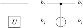
Figure 1: The Feynman notation for the single qubit gate $(\mbox{\bf 1}_{2}\otimes U)$ and for a controlled NOT operation $\left|b_{2}^{\prime}\,b_{1}^{\prime}\right>=\left|b_{2}\,b_{2}\oplus b_{1}\right>$.

A multiply controlled NOT is defined as follows. Let $C$ be a subset of $[1..n]$ not containing the target $t$. Then

$$\mbox{CNOT}_{C,t}\left|x\right>=\left\{\begin{array}[]{ll}\left|y\right>&\mbox{if}\quad b_{c}=1\mbox{ for all }c\in C\\ \left|x\right>&\mbox{otherwise}\end{array}\right.$$

where $\left|y\right>$ is defined as above. Several controlled NOT operations in a sequence allow us to implement the operation $P_{n}\left|x\right>=\left|x+1\bmod 2^{n}\right>$. Note that $O(n)$ elementary gates are sufficient to realize a multiply controlled NOT operation on $n$ qubits, assuming that an additional scratch qubit is available. Therefore, at most $O(n^{2})$ elementary gates are necessary to implement the shift operation $P_{n}$.

Figure 2: Shift

The state of two qubits can be exchanged with the help of three controlled NOT operations:

$$\mbox{SWAP}_{k,h}=\mbox{CNOT}_{h,k}\mbox{CNOT}_{k,h}\mbox{CNOT}_{h,k}.$$

It follows that any permutation of the $n$ quantum wires can be realized with at most $O(n)$ elementary quantum gates.

A more detailed discussion of properties of quantum gates can be found in [1]. We will discuss the construction of the discrete Fourier transform in the next section. In particular, we will show the classical dataflow diagram and the corresponding quantum gates to further illustrate the graphical notation.

§3 Quantum Fourier Transform

The discrete Fourier transform of length $N=2^{n}$ is defined by

$$F_{N}=\frac{1}{\sqrt{N}}\Big{[}\,\omega^{jk}\Big{]}_{j,k=0,\dots,N-1},$$

where $\omega=\exp(2\pi i/N)$ with $i^{2}=-1$. Recall the recursion step used in the Cooley-Tukey decomposition:

$${F_{N}} = \Upsilon_{N}(\mbox{\bf 1}_{2}\otimes F_{N/2})\left(\begin{array}[]{cc}\mbox{\bf 1}_{N/2}&\\ &T_{N/2}\end{array}\right)(F_{2}\otimes\mbox{\bf 1}_{N/2})$$ (3)

where $T_{N/2}:=\mathop{\rm diag}\nolimits(1,\omega,\omega^{2},\dots,\omega^{N/2-1})$ denotes the matrix of twiddle factors, and $\Upsilon_{N}$ denotes the permutation given by $\Upsilon_{N}\left|xb\right>=\left|bx\right>$ with $x$ an $n-1$-bit integer, and $b$ a single bit.

We note that the implementation of $F_{2}$ is a local operation on a single quantum bit. The recursion suggest four different parts of the implementation of Fourier transforms of larger length. The matrix $(F_{2}\otimes\mbox{\bf 1}_{N/2})$ is a single Hadamard operation on the most significant qubit. We would like to emphasize that this single quantum operation corresponds to a full butterfly diagram.

The implementation of the twiddle matrix is more complex. Notice that $T_{N/2}$ can be written as a tensor product of diagonal matrices $L_{j}=\mathop{\rm diag}\nolimits(1,\omega^{2^{j-1}})$ in the form

$$T_{N/2}=L_{n-1}\otimes\dots\otimes L_{2}\otimes L_{1}.$$

Thus, $\mbox{\bf 1}_{N/2}\oplus T_{N/2}$ can be realized by controlled phase shift operations. Figure 3 shows the implementation of the two operations discussed so far.

  

Figure 3: For length N=8, only three qubits are necessary. The circuit on the left implements $(F_{2}\otimes\mbox{\bf 1}_{N/2})$ and the other realizes the twiddle matrix $\mbox{\bf 1}_{4}\oplus\mathop{\rm diag}\nolimits(1,\omega,\omega^{2},\omega^{3})$.

It remains to discuss the other two operations in (3). The operation $(\mbox{\bf 1}_{2}\otimes F_{N/2})$ means that an implementation of the discrete Fourier transform of length $N/2$ is used on the least significant $(n-1)$ bits. The operation $\Upsilon_{N}$ is a permutation of quantum wires. We can combine all the permutations

$$\Upsilon_{N}(\mbox{\bf 1}_{2}\otimes\Upsilon_{N/2})\dots(\mbox{\bf 1}_{N-2}\otimes\Upsilon_{4})$$

into a single permutation of quantum wires. The resulting permutation is the bit reversal, see Figure 4. The classical and quantum implementation of the discrete Fourier transform of length 8 are compared in Figure 5. We observe that the butterfly diagrams find simple realizations but the twiddle matrices require more elementary quantum gate operations.

      

Figure 4: The bit reversal permutation is given by $\mbox{\bf 1}_{2}\otimes\Upsilon_{4}$ followed by $\Upsilon_{8}$.

The complexity of the quantum implementation can be estimated as follows. If we denote by $R(N)$ the number of gates necessary to implement the DFT of length $N=2^{n}$ on a quantum computer, then equation (3) implies the recurrence relation

$$R(N)=R(N/2)+O(\log N)$$

which leads to the estimate $R(N)=O(\log^{2}N)$.

Shor’s factoring algorithm relies on the quantum Fourier transform in a fundamental way. For more details on Fourier transforms and their generalizations to nonabelian groups, see [4, 5].

§4 Quantum Cosine and Sine Transforms

We derive quantum circuits for discrete Cosine and Sine transforms in this section. The main idea is simple: reuse the circuits for the discrete Fourier transform.

The discrete Cosine and Sine transforms are divided into various families. We follow [6] and define the following four versions of discrete Cosine transforms:

$$\begin{array}[]{l@{\quad:=\quad}l}C_{N}^{\rm I}&\left(\displaystyle\frac{2}{N}\right)^{1/2}\left[k_{i}\cos{\displaystyle\frac{ij\pi}{N}}\right]_{i,j=0,\dots,N}\\ C_{N}^{\rm II}&\left(\displaystyle\frac{2}{N}\right)^{1/2}\left[k_{i}\cos{\displaystyle\frac{i(j+1/2)\pi}{N}}\right]_{i,j=0,\dots,N-1}\\ C_{N}^{\rm III}&\left(\displaystyle\frac{2}{N}\right)^{1/2}\left[k_{i}\cos{\displaystyle\frac{(i+1/2)j\pi}{N}}\right]_{i,j=0,\dots,N-1}\\ C_{N}^{\rm IV}&\left(\displaystyle\frac{2}{N}\right)^{1/2}\left[k_{i}\cos{\displaystyle\frac{(i+1/2)(j+1/2)\pi}{N}}\right]_{i,j=0,\dots,N-1}\end{array}$$

where $k_{i}:=1$ for $i=1,\dots,N-1$ and $k_{0}:={1}/{\sqrt{2}}$. The numbers $k_{i}$ ensure that the transforms are orthogonal. The discrete Sine transforms are defined by

$$\begin{array}[]{l@{\quad:=\quad}l}S_{N}^{\rm I}&\left(\displaystyle\frac{2}{N}\right)^{1/2}\left[k_{i}\,\sin{\displaystyle\frac{ij\pi}{N}}\right]_{i,j=1,\dots,N-1}\\ S_{N}^{\rm II}&\left(\displaystyle\frac{2}{N}\right)^{1/2}\left[k_{i}\,\sin{\displaystyle\frac{i(j+1/2)\pi}{N}}\right]_{i,j=0,\dots,N-1}\\ S_{N}^{\rm III}&\left(\displaystyle\frac{2}{N}\right)^{1/2}\left[k_{i}\,\sin{\displaystyle\frac{(i+1/2)j\pi}{N}}\right]_{i,j=0,\dots,N-1}\\ S_{N}^{\rm IV}&\left(\displaystyle\frac{2}{N}\right)^{1/2}\left[k_{i}\,\sin{\displaystyle\frac{(i+1/2)(j+1/2)\pi}{N}}\right]_{i,j=0,\dots,N-1}\end{array}$$

where the constants $k_{i}$ are defined as above. Notice that $C_{N}^{\rm III}$ (resp. $S_{N}^{\rm III}$) is the transpose of $C_{N}^{\rm II}$ (resp. $S_{N}^{\rm II})$, hence it suffices to derive circuits for the type II transforms.

It is well-known that the trigonometric transforms can be obtained by conjugating the discrete Fourier transform $F_{2N}$ by certain sparse matrices. We refer the reader to Wickerhauser [7] for more details on the decompostions.

DCT_I and DST_I.

We derive the circuits for the discrete Sine and Cosine transforms of type I all at once. Indeed, the $\mbox{\rm DST}_{\rm I}$ and $\mbox{\rm DCT}_{\rm I}$ can be recovered from the DFT by a base change

$$T_{N}^{\dagger}\cdot F_{2N}\cdot T_{N}=C_{N}^{\rm I}\oplus iS_{N}^{\rm I},$$ (4)

where

$$T_{N}=\left(\begin{array}[]{rrrrrrrr}1&&&&&&&\\ &\frac{1}{\sqrt{2}}&&&&\frac{i}{\sqrt{2}}&&\\ &&\begin{picture}(5.0,5.0)\put(0.0,4.0){\makebox(0.0,0.0)[]{.}}\put(2.0,2.0){\makebox(0.0,0.0)[]{.}}\put(4.0,0.0){\makebox(0.0,0.0)[]{.}} \end{picture}&&&&\begin{picture}(5.0,5.0)\put(0.0,4.0){\makebox(0.0,0.0)[]{.}}\put(2.0,2.0){\makebox(0.0,0.0)[]{.}}\put(4.0,0.0){\makebox(0.0,0.0)[]{.}} \end{picture}&\\ &&&\frac{1}{\sqrt{2}}&&&&\frac{i}{\sqrt{2}}\\ &&&&\;1&&&\\ &&&\frac{1}{\sqrt{2}}&&&&{-}\frac{i}{\sqrt{2}}\\ &&\begin{picture}(5.0,5.0)\put(0.0,0.0){\makebox(0.0,0.0)[]{.}}\put(2.0,2.0){\makebox(0.0,0.0)[]{.}}\put(4.0,4.0){\makebox(0.0,0.0)[]{.}} \end{picture}&&&&\begin{picture}(5.0,5.0)\put(0.0,0.0){\makebox(0.0,0.0)[]{.}}\put(2.0,2.0){\makebox(0.0,0.0)[]{.}}\put(4.0,4.0){\makebox(0.0,0.0)[]{.}} \end{picture}&\\ &\frac{1}{\sqrt{2}}&&&&{-}\frac{i}{\sqrt{2}}&&\end{array}\right).$$

It is straightforward to check that (4) holds, see Theorem 3.10 in [7]. Since we already know efficient quantum circuits for the DFT, it remains to find an efficient implementation of the base change matrix $T_{N}$.

It will be convenient to denote the basis vectors of ${\mathbf{C}}^{2^{n+1}}$ by $\left|bx\right>$, where $b$ is a single bit and $x$ is an $n$-bit number. The two’s complement of an $n$-bit unsigned integer $x$ is denoted by $x^{\prime}$, that is, $x^{\prime}=2^{n}-x$. The action of $T_{N}$ can be described by

$$\begin{array}[]{lcl@{\qquad\quad}lcl}T_{N}\left|0\mathbf{0}\right>&=&\left|0\mathbf{0}\right>&T_{N}\left|0x\right>&=&\frac{1}{\sqrt{2}}\left|0x\right>+\frac{1}{\sqrt{2}}\left|1x^{\prime}\right>\\[4.30554pt] T_{N}\left|1\mathbf{0}\right>&=&\left|1\mathbf{0}\right>&T_{N}\left|1x\right>&=&\frac{i}{\sqrt{2}}\left|0x\right>-\frac{i}{\sqrt{2}}\left|1x^{\prime}\right>\end{array}$$

for all integers $x$ in the range $1\leq x<2^{n}$. Ignoring the two’s complement in $T_{N}$, we can define an operator $D$ by

$$\begin{array}[]{lcl@{\qquad\quad}lcl}D\left|0\mathbf{0}\right>&=&\left|0\mathbf{0}\right>&D\left|0x\right>&=&\frac{1}{\sqrt{2}}\left|0x\right>+\frac{1}{\sqrt{2}}\left|1x\right>\\[4.30554pt] D\left|1\mathbf{0}\right>&=&\left|1\mathbf{0}\right>&D\left|1x\right>&=&\frac{i}{\sqrt{2}}\left|0x\right>-\frac{i}{\sqrt{2}}\left|1x\right>\end{array}$$

for all integers $x$ in the range $1\leq x<2^{n}$. This operator is essentially block diagonal and easy to implement by a single qubit operation, followed by a correction. Indeed, define the matrix $B$ by $B=\displaystyle\frac{1}{\sqrt{2}}\left(\begin{array}[]{rr}1&i\\ 1&-i\end{array}\right)$, then Figure 5 gives an implementation of the operator $D$.

\begin{picture}(40.0,100.0)\end{picture}

Figure 5: Circuits realizing the block matrix $D$ and the permutation $\pi$.

Define $\pi$ to be the permutation given by a two’s complement conditioned on the most significant bit $\pi\left|0x\right>=\left|0x\right>$ and $\pi\left|1x\right>=\left|1x^{\prime}\right>$ for all $n$-bit integers $x$. It is clear that $T_{N}=\pi D$. The circuits for the permutation $\pi$ is shown in Figure 5.

Theorem 1

The discrete Cosine transform $C_{N}^{\rm I}$ and the discrete Sine transform $S_{N}^{\rm I}$ can be realized with at most $O(\log^{2}N)$ elementary quantum gates; the quantum circuit for these transforms is shown in Figure 6.

Figure 6: Complete quantum circuit for the $\mbox{\rm DCT}_{\rm I}$

Proof. Let $N=2^{n}$. We note that $O(\log^{2}N)$ quantum gates are sufficient to realize the DFT of length $2N$. The permutation $\pi$ can be implemented with at most $O(\log^{2}N)$ elementary gates. At most $O(\log N)$ quantum gates are needed to realize the operator $D$. This shows that the $\mbox{\rm DCT}_{\rm I}$ and the $\mbox{\rm DST}_{\rm I}$ can be realized with at most $O(\log^{2}N)$ quantum gates. The preceding discussion shows that Figure 6 realizes the $\mbox{\rm DCT}_{\rm I}$ and $\mbox{\rm DST}_{\rm I}.$  $\Box$

DCT_IV and DST_IV.

The trigonometric transforms of type IV are derived from the DFT by

$$e^{\pi i/4N}R_{N}^{t}\cdot F_{2N}\cdot R_{N}=C_{N}^{\rm IV}\oplus(-i)S_{N}^{\rm IV}.$$ (5)

Here $R_{N}$ denotes the matrix

$$R_{N} = \frac{1}{\sqrt{2}}\left(\begin{array}[]{cccccccc}1&&&&-i&&&\\ &\omega&&&&-i\omega&&\\ &&\begin{picture}(5.0,5.0)\put(0.0,4.0){\makebox(0.0,0.0)[]{.}}\put(2.0,2.0){\makebox(0.0,0.0)[]{.}}\put(4.0,0.0){\makebox(0.0,0.0)[]{.}} \end{picture}&&&&\begin{picture}(5.0,5.0)\put(0.0,4.0){\makebox(0.0,0.0)[]{.}}\put(2.0,2.0){\makebox(0.0,0.0)[]{.}}\put(4.0,0.0){\makebox(0.0,0.0)[]{.}} \end{picture}&\\ &&&\omega^{N-1}&&&&-i\omega^{N-1}\\ &&&\overline{\omega}^{N}&&&&1\\ &&\begin{picture}(5.0,5.0)\put(0.0,4.0){\makebox(0.0,0.0)[]{.}}\put(2.0,6.0){\makebox(0.0,0.0)[]{.}}\put(4.0,8.0){\makebox(0.0,0.0)[]{.}} \end{picture}&&&&\begin{picture}(5.0,5.0)\put(0.0,4.0){\makebox(0.0,0.0)[]{.}}\put(2.0,6.0){\makebox(0.0,0.0)[]{.}}\put(4.0,8.0){\makebox(0.0,0.0)[]{.}} \end{picture}&\\ &\overline{\omega}^{2}&&&&i\overline{\omega}^{2}&&\\ \overline{\omega}&&&&i\overline{\omega}&&&\\ \end{array}\right)$$

with $\omega$ the primitive $4N$-th root of unity $\omega=\exp(2\pi i/4N)$. Equation (5) is a consequence of Theorem 3.19 in [7] obtained by complex conjugation.

Theorem 2

The discrete Cosine transform $C_{N}^{\rm IV}$ and the discrete Sine transform $S_{N}^{\rm IV}$ can be realized with at most $O(\log^{2}N)$ elementary quantum gates; the quantum circuit for these transforms is shown in Figure 7.

Figure 7: Complete quantum circuit for $\mbox{\rm DCT}_{\rm IV}$

Proof. It remains to show that there exists an efficient quantum circuit for the matrix $R_{N}$ in equation (5). A factorization of $R_{N}$ can be obtained as follows. Denote by $\overline{x}$ the one’s complement of an $n$-bit integer $x$. We define a permutation matrix $\pi_{1}$ by $\pi_{1}\left|0x\right>=\left|0x\right>$ and $\pi_{1}\left|1x\right>=\left|1\overline{x}\right>$ for all integers $x$ in the range of $0\leq x<2^{n}$. Denote by $D_{1}$ the diagonal matrix

$$D_{1}={\rm diag}(1,\omega,\dots,\omega^{N-1},\overline{\omega}^{N},\dots,\overline{\omega}^{2},\overline{\omega}).$$

Then $R_{N}$ can be factored as

$$R_{N} = \pi_{1}\cdot D_{1}\cdot\left(\frac{1}{\sqrt{2}}\left(\begin{array}[]{rr}1&-i\\ 1&i\end{array}\right)\otimes\mbox{\bf 1}_{N}\right)=\pi_{1}\cdot D_{1}\cdot(\overline{B}\otimes\mbox{\bf 1}_{N}).$$

Note that $\overline{B}\otimes\mbox{\bf 1}_{N}$ is a single qubit operation, and $\pi_{1}$ can be realized by controlled not operations. The implementation of the diagonal matrix $D_{1}$ is more interesting. Note that the diagonal matrices of increasing (decreasing) powers can be written by tensor products

$$\begin{array}[]{lcl}\Delta_{1}=\mathop{\rm diag}\nolimits(1,\omega,\dots,\omega^{N-1})&=&L_{n}\otimes\cdots\otimes L_{2}\otimes L_{1}\\ \Delta_{2}=\mathop{\rm diag}\nolimits(\overline{\omega}^{N-1},\dots,\overline{\omega},1)&=&K_{n}\otimes\cdots\otimes K_{2}\otimes K_{1}\end{array}$$

where $L_{j}=\mathop{\rm diag}\nolimits(1,\omega^{2^{j-1}})$ and $K_{j}=\mathop{\rm diag}\nolimits(\overline{\omega}^{\,2^{j-1}},1)$. Therefore, it is possible to write $D_{1}$ in the form $D_{1}=(C\otimes\mbox{\bf 1}_{N})\cdot(\Delta_{1}\oplus\Delta_{2})$ with $C=\mathop{\rm diag}\nolimits(1,\overline{\omega})$. The circuit for the diagonal matrix $D_{1}$ is shown in Figure 8.

Figure 8: Quantumcircuit for the diagonal matrix $D_{1}$.

The complete quantum circuit for the DCT_IV is shown in Figure 7. Note that the last three single qubit gates $C$, $B^{\dagger}$, and $M=\mathop{\rm diag}\nolimits(e^{\pi i/4N},e^{\pi i/4N})$ can be combined into a single gate $MB^{\dagger}C$.  $\Box$

DCT_II and DST_II.

The implementation of the trigonometric transforms of type II follows a similar pattern. Both transforms can be recovered from the DFT of length 2N after multiplication with certain sparse matrices, cf. Theorem 3.13 in [7]:

$$U_{N}^{\dagger}\cdot F_{2N}\cdot V_{N}=C_{N}^{\rm II}\oplus(-i)S_{N}^{\rm II},$$ (8)

where

$$V_{N}=\frac{1}{\sqrt{2}}\left(\begin{array}[]{rrrrrr}1&&&1&&\\ &\begin{picture}(5.0,5.0)\put(0.0,4.0){\makebox(0.0,0.0)[]{.}}\put(2.0,2.0){\makebox(0.0,0.0)[]{.}}\put(4.0,0.0){\makebox(0.0,0.0)[]{.}} \end{picture}&&&\begin{picture}(5.0,5.0)\put(0.0,4.0){\makebox(0.0,0.0)[]{.}}\put(2.0,2.0){\makebox(0.0,0.0)[]{.}}\put(4.0,0.0){\makebox(0.0,0.0)[]{.}} \end{picture}&\\ &&1&&&\phantom{-}1\\ &&1&&&-1\\ &\begin{picture}(5.0,5.0)\put(0.0,4.0){\makebox(0.0,0.0)[]{.}}\put(2.0,6.0){\makebox(0.0,0.0)[]{.}}\put(4.0,8.0){\makebox(0.0,0.0)[]{.}} \end{picture}&&&\begin{picture}(5.0,5.0)\put(0.0,4.0){\makebox(0.0,0.0)[]{.}}\put(2.0,6.0){\makebox(0.0,0.0)[]{.}}\put(4.0,8.0){\makebox(0.0,0.0)[]{.}} \end{picture}&\\ 1&&&-1&&\end{array}\right)$$

and

$$U_{N}=\left(\begin{array}[]{cccccccc}1&&&&0&&&\\ &\frac{\overline{\omega}}{\sqrt{2}}&&&{-}\frac{i\overline{\omega}}{\sqrt{2}}&\begin{picture}(5.0,5.0)(-20.0,10.0)\put(0.0,4.0){\makebox(0.0,0.0)[]{.}}\put(2.0,2.0){\makebox(0.0,0.0)[]{.}}\put(4.0,0.0){\makebox(0.0,0.0)[]{.}} \end{picture}&&\\ &&\begin{picture}(5.0,5.0)\put(0.0,4.0){\makebox(0.0,0.0)[]{.}}\put(2.0,2.0){\makebox(0.0,0.0)[]{.}}\put(4.0,0.0){\makebox(0.0,0.0)[]{.}} \end{picture}&&&\begin{picture}(5.0,5.0)\put(0.0,4.0){\makebox(0.0,0.0)[]{.}}\put(2.0,2.0){\makebox(0.0,0.0)[]{.}}\put(4.0,0.0){\makebox(0.0,0.0)[]{.}} \end{picture}&&\\ &&&\frac{\overline{\omega}^{N-1}}{\sqrt{2}}&&&{-}\frac{i\overline{\omega}^{N-1}}{\sqrt{2}}&0\\ &&&0&&&&-1\\ &&\begin{picture}(5.0,5.0)(10.0,10.0)\put(0.0,0.0){\makebox(0.0,0.0)[]{.}}\put(2.0,2.0){\makebox(0.0,0.0)[]{.}}\put(4.0,4.0){\makebox(0.0,0.0)[]{.}} \end{picture}&\frac{\omega^{N-1}}{\sqrt{2}}&&&\frac{i\omega^{N-1}}{\sqrt{2}}&\\ &&\begin{picture}(5.0,5.0)\put(0.0,0.0){\makebox(0.0,0.0)[]{.}}\put(2.0,2.0){\makebox(0.0,0.0)[]{.}}\put(4.0,4.0){\makebox(0.0,0.0)[]{.}} \end{picture}&&&\begin{picture}(5.0,5.0)\put(0.0,0.0){\makebox(0.0,0.0)[]{.}}\put(2.0,2.0){\makebox(0.0,0.0)[]{.}}\put(4.0,4.0){\makebox(0.0,0.0)[]{.}} \end{picture}&&\\ 0&\frac{\omega}{\sqrt{2}}&&&\frac{i\omega}{\sqrt{2}}&&&\end{array}\right),$$

and $\omega$ denotes the $4N$-th primitive root of unity $\omega=\exp(2\pi i/4N)$, $i^{2}=-1$.

Theorem 3

The discrete Cosine transform $C_{N}^{\rm II}$ and the discrete Sine transform $S_{N}^{\rm II}$ can be realized with at most $O(\log^{2}N)$ elementary quantum gates; the quantum circuit for these transforms is shown in Figure 9.

Figure 9: Complete quantum circuit for $\mbox{\rm DCT}_{\rm II}$

Proof. We need to derive efficient quantum circuits for the matrices $V_{N}$ and $U_{N}$ in equation (8). The matrix $V_{N}$ has a fairly simple decomposition in terms of quantum circuits.

Lemma 4

$V_{N}=\pi_{1}(H\otimes\mbox{\bf 1}_{N})$.

Proof. It is clear that the Hadamard transform on the most significant bit $H\otimes I_{N}$ is – up to a permutation of rows – equivalent to $V_{N}$. The appropriate permutation of rows has been introduced in the previous section, namely $\pi_{1}\left|0x\right>=\left|1x\right>$ and $\pi_{1}\left|1x\right>=\left|1\overline{x}\right>$ for all $0\leq x<2^{n}$. We can conclude that $V_{N}=\pi_{1}(H\otimes\mbox{\bf 1}_{N})$ as desired.  $\Box$

The decomposition of $U_{N}$ is more elaborate. Notice that

$$\begin{array}[]{l@{\qquad\!}l}U_{N}\left|0\mathbf{0}\right>=\left|0\mathbf{0}\right>&U_{N}\left|0x\right>=\displaystyle\frac{\overline{\omega}^{\,x}}{\sqrt{2}}\left|0x\right>+\frac{\omega^{x}}{\sqrt{2}}\left|1x^{\prime}\right>\\ U_{N}\left|1\mathbf{1}\right>=(-1)\left|1\mathbf{0}\right>&U_{N}\left|1y\right>=\displaystyle-\frac{i\overline{\omega}^{\,y+1}}{\sqrt{2}}\left|0\,(y+1\bmod 2^{n})\right>+\frac{i\omega^{y+1}}{\sqrt{2}}\left|1\overline{y}\right>\end{array}$$

for all integers $x$ in the range $1\leq x<2^{n}$ and all integers $y$ in $0\leq y<2^{n}-1$. Here $\mathbf{0}$ and $\mathbf{1}$ denote the $n$-bit integers $0$ and $2^{n}-1$ respectively.

Define $D_{0}$ by $D_{0}\left|1\mathbf{0}\right>=i\left|1\mathbf{0}\right>$ and $D_{0}\left|x\right>=\left|x\right>$ otherwise. We define a permutation $\pi_{2}$ by $\pi_{2}\left|0x\right>=\left|0x\right>$ and $\pi_{2}\left|1x\right>=\left|1(x+1\bmod 2^{n})\right>$ for all integers $x$ in $0\leq x<2^{n}$.

Lemma 5

$U_{N}=D_{1}^{\dagger}\,\overline{T}_{N}\,D_{0}^{\phantom{\dagger}}\,\pi_{2}$.

Proof. Since $D_{1}^{\dagger}\left|0x\right>=\overline{\omega}^{x}\left|0x\right>$ and $D_{1}^{\dagger}\left|1x\right>=\omega^{\,x^{\prime}}\left|1x\right>$, we obtain

$$\begin{array}[]{l}D_{1}^{\dagger}\overline{T}_{N}\left|0x\right>=\displaystyle\phantom{-}\frac{\overline{\omega}^{x}}{\sqrt{2}}\left|0x\right>+\frac{\omega^{x}}{\sqrt{2}}\left|1x^{\prime}\right>\\[8.61108pt] D_{1}^{\dagger}\overline{T}_{N}\left|1x\right>=\displaystyle-\frac{i\overline{\omega}^{x}}{\sqrt{2}}\left|0x\right>+\frac{i\omega^{x}}{\sqrt{2}}\left|1x^{\prime}\right>\end{array}$$

We have $D_{0}\pi_{2}\left|0x\right>=\left|0x\right>$, $D_{0}\pi_{2}\left|1x\right>=\left|1(x+1\bmod 2^{n})\right>$ for all integers $x$ in $0\leq x<2^{n}-1$, and $D_{0}\pi_{2}\left|1\mathbf{1}\right>=i\left|1\mathbf{0}\right>$. We note that $(x+1\bmod 2^{n})^{\prime}=\overline{x}$, whence combining $D_{1}\overline{T}_{N}$ with $D_{0}\pi_{2}$ shows the result.  $\Box$

Recall that $T_{N}=\pi D$. It follows that

$$U_{N}^{\dagger}=\pi_{2}^{-1}(\overline{D}_{0}D^{t})\pi^{-1}D_{1}.$$

The implementation of $D_{1}$ has been described in the section on the DCT_IV, and the implementation of $\pi$ (and hence $\pi^{-1}$) is contained in the section on the DCT_I. The implementation of $\pi_{2}^{-1}$ is also straightforward. It remains to find an implementation of $\overline{D}_{0}D^{t}$. We observe that

$$\begin{array}[]{lcl@{\qquad\quad}lcl}\overline{D}_{0}D^{t}\left|0\mathbf{0}\right>&=&\phantom{(-i)}\left|0\mathbf{0}\right>&\overline{D}_{0}D^{t}\left|0x\right>&=&\frac{1}{\sqrt{2}}\left|0x\right>+\frac{i}{\sqrt{2}}\left|1x\right>\\[4.30554pt] \overline{D}_{0}D^{t}\left|1\mathbf{0}\right>&=&(-i)\left|1\mathbf{0}\right>&\overline{D}_{0}D^{t}\left|1x\right>&=&\frac{1}{\sqrt{2}}\left|0x\right>-\frac{i}{\sqrt{2}}\left|1x\right>\end{array}$$

This can be accomplished by the single bit operation $B^{t}\otimes\mbox{\bf 1}_{N}$ followed by a multiply conditioned gate $J=\displaystyle\frac{1}{\sqrt{2}}\left(\begin{array}[]{rr}1&-i\\ -i&1\end{array}\right)$. The full circuit is shown in Figure 9. The statement about the complexity is clear.  $\Box$

§5 Quantum Hartley Transforms

The discrete Hartley transform of length $N\in{\mathbf{N}}$ is the real $N\times N$ matrix $A_{N}$ defined by

$$A_{N}:=\frac{1}{\sqrt{N}}\Big{[}{\rm cas}\Big{(}\frac{2\pi ij}{N}\Big{)}\Big{]}_{i,j=0,\ldots,N-1},$$

where the function ${\rm cas}:{\mathbf{R}}\rightarrow{\mathbf{R}}$ is defined by ${\rm cas}(x):=\cos(x)+\sin(x)$, see [2, 3] for classical implementations. The property

$$A_{N}=\left(\frac{1-i}{2}\right)\;F_{N}+\left(\frac{1+i}{2}\right)\;F_{N}^{3}$$

is easily seen from the definition. We derive a quantum circuit implementing $A_{N}$ with one auxiliary quantum bit.

  

Figure 10: Circuit realising a quantum Hartley transform

Lemma 6

The discrete Hartley transform can be factorized in the form shown in Figure 10. Here $R$ is the unitary circulant matrix

$$R:=\frac{1}{2}\left(\begin{array}[]{rr}1-i&1+i\\ 1+i&1-i\end{array}\right)$$

and $H$ denotes the Hadamard transform.

Proof. Let $\check{F}_{N}$ be the transformation which effects a DFT conditioned to the first bit, i. e., written in terms of matrices we have $\check{F}_{N}=\mbox{\bf 1}_{N}\oplus F_{N}$. We now show that the given circuit computes the linear transformation $\left|0\right>\left|x\right>\mapsto\left|0\right>A_{N}\left|x\right>$ for all unit vectors $x\in{\mathbf{C}}^{n}$. Proceeding from left to right in the circuit given in Figure 10 we obtain

$$\left|0\right>\left|x\right> \stackrel{{\scriptstyle H}}{{\longmapsto}} \frac{1}{\sqrt{2}}(\left|0\right>+\left|1\right>)\left|x\right>$$

$$\stackrel{{\scriptstyle F_{N}}}{{\longmapsto}} \frac{1}{\sqrt{2}}(\left|0\right>+\left|1\right>)F_{N}\left|x\right>$$

$$\stackrel{{\scriptstyle\check{F}_{N}^{2}}}{{\longmapsto}} \frac{1}{\sqrt{2}}\left|0\right>F_{N}\left|x\right>+\frac{1}{\sqrt{2}}\left|0\right>F_{N}^{3}\left|x\right>$$

$$\stackrel{{\scriptstyle R}}{{\longmapsto}} \frac{1}{\sqrt{2}}\left|0\right>\left(\frac{1}{2}(1-i)F_{N}+\frac{1}{2}(1+i)F_{N}^{3}\right)\left|x\right>$$

$$+\frac{1}{\sqrt{2}}\left|1\right>\left(\frac{1}{2}(1+i)F_{N}+\frac{1}{2}(1-i)F_{N}^{3}\right)\left|x\right>$$

$$= \frac{1}{\sqrt{2}}\left|0\right>A_{N}\left|x\right>+\frac{1}{\sqrt{2}}\left|1\right>F_{N}^{-2}A_{N}\left|x\right>$$

$$\stackrel{{\scriptstyle\check{F}_{N}^{2}}}{{\longmapsto}} \frac{1}{\sqrt{2}}(\left|0\right>+\left|1\right>)A_{N}\left|x\right>$$

$$\stackrel{{\scriptstyle H}}{{\longmapsto}} \left|0\right>A_{N}\left|x\right>$$

as desired.  $\Box$

Theorem 7

The discrete Hartley transform $A_{N}$ can be computed on a quantum computer using $O(\log^{2}N)$ elementary operations if we allow one additional ancilla qubit.

Proof. Recall that the discrete Fourier transform $F_{N}$ can be implemented $O(\log^{2}N)$ operations as shown in Section §3. The statement follows from Lemma 6 since all transformations given there require at most $O(\log^{2}N)$ elementary operations.  $\Box$

§6 Conclusions

We have shown that the discrete Cosine transforms, the discrete Sine transforms, and the discrete Hartley transforms have extremely efficient realizations on a quantum computer. All implementations illustrated an important design principle: the reusability of highly optimized quantum circuits. Apart from a few sparse matrices, we only needed the circuits for the discrete Fourier transform for the implementations. A key point is that an improvement of a basic circuit, like the DFT, immediately leads to more efficient quantum circuits for the DCT, DST, and DHT.

References

• [1] A. Barenco, C. H. Bennett, R. Cleve, D. P. DiVincenzo, N. Margolus, P. Shor, T. Sleator, J. A. Smolin, and H. Weinfurter. Elementary gates for quantum computation. Physical Review A, 52(5):3457–3467, November 1995.
• [2] Th. Beth. Generating Fast Hartley Transforms - Another Application of the Algebraic Discrete Fourier Transform. In Proc. URSI-ISSSE ’89, pages 688–692, 1989.
• [3] Bracewell. The Hartley Transform. Cambridge Univ. Press, 1979.
• [4] P. Høyer. Efficient Quantum Transforms. LANL preprint quant–ph/9702028, February 1997.
• [5] M. Püschel, M. Rötteler, and Th. Beth. Fast Quantum Fourier Transforms for a Class of non-abelian Groups. In Proceedings Applied Algebra, Algebraic Algorithms and Error-Correcting Codes (AAECC-13), volume 1719 of Lecture Notes in Computer Science, pages 148–159. Springer, 1999.
• [6] K. R. Rao and P. Yip. Discrete Cosine Transform: Algorithms, Advantages, and Applications. Academic Press, 1990.
• [7] V. Wickerhauser. Adapted Wavelet Analysis from Theory to Software. A.K. Peters, Wellesley, 1993.