Temporal Windowing of Trapped States

Abstract

Trapped state definition for 3-level atoms in $\Lambda$ configuration, is a very restrictive one, and for the case of unpolarized beams, this definition no longer holds. We introduce a more general definition by using a reference frame rotating with the frequency of the control field, obtaining a temporal windowing for the trapped population. This amounts to a time quantization of the coherent population transfer, making possible to study the phase coherence in trapped light PACS number(s): 32.50.+d, 32.80.Qk, 32.80.-t

I Introduction

3D vector representation had become an important tool in the handling and understanding of 3-level atoms. News phenomena such as dark states, electromagnetic induced transparency (EIT) Har , coherent population transfer (CPT)sho kn , and the very recent introduction of polaritonsfle1 to explain the ”capture and storing of light in Cslau and ${}^{87}Rb$fle2 are easily understood in the framework of a geometric representation for 3D vector model. In particular the so named $\Lambda$ configuration with the two close lying ground states in non allowed Raman transitions had been largely considered in adiabatic Raman interactions shk and a geometric representation have been proposed. A usual way of doing vector models in quantum optics begin with the Maxwell-Bloch equations for the 2-level atoms. In this case the achieving of a 3D vector representation is immediate with components $J_{x},J_{y}$ and $J_{z}$ having a clear physical meaning: the polarization being $P=J_{x}+iJ_{y}$ and $J_{z}$ the population inversion (FIG.1). For 3-level atoms similar geometric representation can be obtained. In this approach, interaction with two different optical fields are considered (geometrically) as the sum of two levels atom-field interaction, each field coupling two different levels independly. However this approach clearly lacks in rigourously since it is based on the assumption that addition of two level geometric (the SU(2) Isospin )representation describes exactly well the three levels atom-field dynamics (SU(3)Isospin); however it works quite well in 3-level atoms with $\Lambda$ configuration where the two grounds levels are close lying.

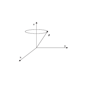
Figure 1: The vector polarization $J\textbf{J}$ rotating with frequency $\Omega$.

II Basic ideas

In the following, we briefly review the basic ideas involved in this approach. The time evolution of vectors like angular momentum (for example magnetic momentum) is given by:

$$\frac{dJ}{dt}=J\times\Omega.$$ (1)

This equation describes the precession of vector $J$, around $\Omega$ axis. A very important fact is that any physical quantity satisfying EQ.(1) it is precesing in space as shown in FIG. 1. For two level atoms the geometric representation for the Bloch equations is immediate and comparison with EQ.(1) allows us identify the geometric rotation frequencies with physical quantities: $\Omega_{x}=0$, $\Omega_{y}=2ga$, $\Omega_{z}=\triangle$.

Following this line of thinking, we write down in what follows, the Maxwell-Bloch equations for the the 3-level atoms, in $\Lambda$ configuration (FIG.2 and pursuit identical identification as for the 2-level case. The hamiltonian for 3-level atoms can be written as

$$\mathbf{H} = \mathbf{a}_{1}\mathbf{a}_{1}^{{\dagger}}\hbar\omega_{1}+\mathbf{a}_{2}\mathbf{a}_{2}^{{\dagger}}\hbar\omega_{2}$$ (2)

$$+ \mathbf{J}_{22}\hbar\omega_{21}+\mathbf{J}_{33}\hbar\omega_{31}$$

$$+ g_{1}(\mathbf{a}_{1}\mathbf{J}_{21}+\mathbf{a}_{1}^{{\dagger}}\mathbf{J}_{12})+g_{2}(\mathbf{a}_{2}\mathbf{J}_{32}+\mathbf{a}_{2}^{{\dagger}}\mathbf{J}_{23})$$

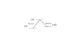
Figure 2: 3level atom in $\Lambda$ configuration with very close lying ground states levels. $E_{1}(z,t)$ is the control field and $E_{2}(z,t)$ is the signal field

where $g_{1}=\mu_{13}\sqrt{\frac{\hbar\omega_{1}}{\epsilon_{0}V}}$, and $g_{2}=\mu_{23}\sqrt{\frac{\hbar\omega_{23}}{\epsilon_{0}V}}$ represent the atom-field intensity coupling of transitions 1 $\Leftrightarrow$ 3 and 2 $\Leftrightarrow$ 3 respectively, and $\mathbf{a_{1},a_{2}}$ are the optical fields with frequencies $w_{1}$, and $w_{2}$ associated with those transitions. As usual $\mathbf{J_{nm}}$ are the collective atoms raiser ($n>m$) or lower ($n<m$) operators. The Maxwell-Bloch equations are then obtained by solving the Heisenberg motion equation $i\hbar\dot{\mathbf{O}}=[\mathbf{O},\mathbf{H}]$, performing R.W.A in the $\mathbf{a_{1}}$ optical field (taking rotating reference system with $w_{1}$ frequency) and phenomenological addition of the decaying terms

$$\mathbf{\dot{J}_{33}} = -\frac{ig_{1}}{\hbar}(\mathbf{a_{1}J_{31}-a_{1}^{\dagger}J_{13}})-\frac{ig_{2}}{\hbar}(\mathbf{a_{2}J_{32}-a_{2}^{\dagger}J_{23}})$$

$$-(\Gamma_{13}+\Gamma_{23})\mathbf{J}_{33}$$

$$\mathbf{\dot{J}_{22}} = \frac{ig_{2}}{\hbar}(\mathbf{a_{2}J_{32}-a_{2}^{\dagger}J_{23}})+\Gamma_{23}\mathbf{J}_{33}$$

$$\mathbf{\dot{J}_{11}} = \frac{ig_{1}}{\hbar}(\mathbf{a_{1}J_{31}-a_{1}^{\dagger}J_{13}})+\Gamma_{13}\mathbf{J}_{33}$$

$$\mathbf{\dot{J}_{13}} = i\delta_{1}\mathbf{J_{13}}-\frac{ig_{1}}{\hbar}\mathbf{a_{1}\Delta_{13}}-\frac{ig_{2}}{\hbar}\mathbf{a_{2}J_{12}}-\gamma_{13}\mathbf{J}_{13}$$

$$\mathbf{\dot{J}_{23}} = i(\delta_{1}+\omega_{21})\mathbf{J_{23}}-\frac{ig_{1}}{\hbar}\mathbf{a_{1}J_{21}}-\frac{ig_{2}}{\hbar}\mathbf{a_{2}\Delta_{23}}-\gamma_{23}\mathbf{J}_{23}$$

$$\mathbf{\dot{J}_{12}} = i\delta_{2}\mathbf{J_{12}}+\frac{ig_{1}}{\hbar}\mathbf{a_{1}J_{32}}-\frac{ig_{2}}{\hbar}\mathbf{a_{2}^{\dagger}J_{13}}-\gamma_{12}\mathbf{J}_{12}$$

Where :

$$\mathbf{\Delta_{13}}=\mathbf{J_{11}-{J_{33}}},\ \ \mathbf{\Delta_{23}}=\mathbf{J_{22}-{J_{33}}}$$

$$\delta_{1}=\omega_{1}-\omega_{31},\ \ \delta_{2}=\omega_{1}-\omega_{21}$$

and $\gamma_{ij}$, $\Gamma_{ij}$ are the decaying constants for polarizations and excitations respectively

In order to get a geometric representation we will assume the system prepared in a convenient experimental set up as to have a common $Z$ axis; furthermore we write down for the polarizations $J_{nm}=J_{x}^{nm}-iJ_{y}^{nm}$, if $n>m$ and similarly for the optical fields $a^{n}=a^{n}_{x}-ia^{n}_{y}$ replacing in equation (3) and making $g_{1}=\hbar\ \bar{g}_{1}$ :

$$\dot{\mathbf{J}}_{x}^{12} = \bar{g_{2}}(\mathbf{a}_{2}^{x}\mathbf{J}_{y}^{13}+\mathbf{a}_{2}^{y}\mathbf{J}_{x}^{13})+\bar{g_{1}}\mathbf{a}_{1}^{x}\mathbf{J}_{y}^{23}-\delta_{2}\mathbf{J}_{y}^{12}-\gamma_{12}\mathbf{J}_{x}^{12}$$

$$\dot{\mathbf{J}}_{y}^{12} = \delta_{2}\mathbf{J}_{x}^{12}+\bar{g_{1}}\mathbf{a}_{1}^{x}\mathbf{J}_{x}^{23}-\bar{g_{2}}(\mathbf{a}_{2}^{x}\mathbf{J}_{x}^{13}-\mathbf{a}_{2}^{y}\mathbf{J}_{y}^{13})-\gamma_{12}\mathbf{J}_{y}^{12}$$

$$\dot{\mathbf{J}}_{z}^{12} = 2\bar{g_{1}}\mathbf{a}_{1}^{x}\mathbf{J}_{y}^{13}-2\bar{g_{2}}(\mathbf{a}_{2}^{x}\mathbf{J}_{y}^{23}+\mathbf{a}_{2}^{y}\mathbf{J}_{x}^{23})$$ (4)

$$+(\Gamma_{13}-\Gamma_{23})\mathbf{J}_{33}$$

$$\dot{\mathbf{J}}_{x}^{13} = \bar{g_{2}}(\mathbf{a}_{2}^{x}\mathbf{J}_{y}^{12}-\mathbf{a}_{2}^{y}\mathbf{J}_{x}^{12})-\delta_{1}\mathbf{J}_{y}^{13}-\gamma_{13}\mathbf{J}_{x}^{13}$$

$$\dot{\mathbf{J}}_{y}^{13} = \delta_{1}\mathbf{J}_{x}^{13}-\bar{g_{1}}\mathbf{a}_{1}^{x}\Delta_{13}-\bar{g_{2}}(\mathbf{a}_{2}^{x}\mathbf{J}_{x}^{12}+\mathbf{a}_{2}^{y}\mathbf{J}_{y}^{12})-\gamma_{13}\mathbf{J}_{y}^{13}$$

$$\dot{\mathbf{J}}_{z}^{13} = 4\bar{g_{1}}\mathbf{a}_{1}^{x}\mathbf{J}_{y}^{13}+2\bar{g_{2}}(\mathbf{a}_{2}^{x}\mathbf{J}_{y}^{23}+\mathbf{a}_{2}^{y}\mathbf{J}_{x}^{23})$$ (5)

$$+(2\Gamma_{13}+\Gamma_{23})\mathbf{J}_{33}$$

$$\dot{\mathbf{J}}_{x}^{23} = -(\delta_{1}+\omega_{21})\mathbf{J}_{y}^{23}-\bar{g_{1}}\mathbf{a}_{1}^{x}\mathbf{J}_{y}^{12}-\bar{g_{2}}\mathbf{a}_{2}^{y}\mathbf{\Delta}_{23}-\gamma_{23}\mathbf{J}_{x}^{23}$$

$$\dot{\mathbf{J}}_{y}^{23} = (\delta_{1}+\omega_{21})\mathbf{J}_{x}^{23}-\bar{g_{1}}\mathbf{a}_{1}^{x}\mathbf{J}_{x}^{12}-\bar{g_{2}}\mathbf{a}_{2}^{x}\mathbf{\Delta}_{23}-\gamma_{23}\mathbf{J}_{y}^{23}$$

$$\dot{\mathbf{J}}_{z}^{23} = 2\bar{g_{1}}\mathbf{a}_{1}^{x}\mathbf{J}_{y}^{13}+4\bar{g_{2}}(\mathbf{a}_{2}^{x}\mathbf{J}_{y}^{23}+\mathbf{a}_{2}^{y}\mathbf{J}_{x}^{23})$$ (6)

$$+(\Gamma_{13}+2\Gamma_{23})\mathbf{J}_{33}$$

The construction of vector $\mathbf{J}$

The construction of a geometric vector representation is done by considering $\omega_{21}<<\omega_{31},\omega_{23}$. This mean that in the absence of any optical field coupling the transition $1\Leftrightarrow 2$, the contribution of this transition in the absorbtion of photons from the optical fields, which is due to imaginary part $\mathbf{J}_{y}^{12}$ is neglected and the same can be argued for the diffractive part $\mathbf{J}_{x}^{12}$. We could say then that in the overall dynamic of the vector polarization $\mathbf{J}$, the influence of $\mathbf{J}_{12}$ is negligible. we do not need to consider the role of spontaneous emission since for any dark state the relaxation rate $\Gamma$ is very smallhus(below 3kHz for sodium). With this approach EQ. (5) and (6) are now:

$$\dot{\mathbf{J}}_{x}^{13} = -\delta_{1}\mathbf{J}_{y}^{13}$$

$$\dot{\mathbf{J}}_{y}^{13} = \delta_{1}\mathbf{J}_{x}^{13}-\bar{g_{1}}\mathbf{a}_{1}^{x}\Delta_{13}$$

$$\dot{\mathbf{J}}_{z}^{13} = 4\bar{g_{1}}\mathbf{a}_{1}^{x}\mathbf{J}_{y}^{13}+2\bar{g_{2}}(\mathbf{a}_{2}^{x}\mathbf{J}_{y}^{23}+\mathbf{a}_{2}^{y}\mathbf{J}_{x}^{23})$$ (7)

$$\dot{\mathbf{J}}_{x}^{23} = -(\delta_{1}+\omega_{21})\mathbf{J}_{y}^{23}-\bar{g_{2}}\mathbf{a}_{2}^{y}\mathbf{\Delta}_{23}$$

$$\dot{\mathbf{J}}_{y}^{23} = (\delta_{1}+\omega_{21})\mathbf{J}_{x}^{23}-\bar{g_{2}}\mathbf{a}_{2}^{x}\mathbf{\Delta}_{23}$$

$$\dot{\mathbf{J}}_{z}^{23} = 2\bar{g_{1}}\mathbf{a}_{1}^{x}\mathbf{J}_{y}^{13}+4\bar{g}_{2}(\mathbf{a}_{2}^{x}\mathbf{J}_{y}^{23}+\mathbf{a}_{2}^{y}\mathbf{J}_{x}^{23})$$ (8)

Identification of Rabbi frequencies are immediate for each transition: $\Omega_{z}^{13}=\delta_{1}$, $\Omega_{x}^{13}=4\bar{g}_{1}\mathbf{a}_{1}^{x}$ and $\Omega_{y}^{13}=0$, for the $1\Leftrightarrow 3$ and $\Omega_{z}^{23}=(\delta_{1}+\omega_{21})$, $\Omega_{x}^{23}=4\bar{g_{2}}\mathbf{a}_{2}^{x}$, $\Omega_{y}^{23}=4\bar{g_{2}}\mathbf{a}_{2}^{y}$ for the $2\Leftrightarrow 3$ transition. The resulting (7) and (8) equations, are easily interpreted geometrically recognizing:

$$\Omega_{x}^{23} = 4\bar{g_{2}}\mathbf{a}_{2}\cos\Delta t$$

$$\Omega_{y}^{23} = 4\bar{g_{2}}\mathbf{a}_{2}\sin\Delta t$$ (9)

where we have defined the field detunings $\Delta=\omega_{1}-\omega_{2}$.

Since R.W.A have been made choosing a reference frame system which is rotating with the $\omega_{1}$ frequency,the field $a_{2}$ it appears as rotating with $\Delta$ frequency, we also have choose, as usual, the imaginary part of $a_{1}$ in the Rotating system equal to cero. The FIG. 3 represent the geometric realization of the whole dynamic for the 3-level atoms in the framework of non allowed raman transitions (or very close-lying levels)

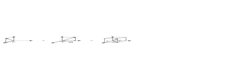
Figure 3: The FIG. at the right hand side represents the polarization of 3-level atom considered as addition of 2level atoms polarization when interaction $1\Leftrightarrow 2$ is neglected

III Redefining Trapped States

The customary trapped state definition is given as

$$\mid-> = \cos\theta\mid 1>-\sin\theta\mid 2>$$

$$\mid+> = \sin\theta\mid 1>+\cos\theta\mid 2>$$ (10)

with $\sin\theta=\frac{g_{1}}{g}$ and $\cos\theta=\frac{g_{2}}{g}$, where $g=\sqrt{g_{1}^{2}+g_{2}^{2}}$.

Definition (10) corresponds to a similarity transformations around Z axis. Clearly, the geometric interpretation can be taken as a summation of the two isospin realization for the case of two levels atoms, with the two fields falling orthogonal to the atom and no coupling between levels $1\Leftrightarrow 2$. We find this definition a very restrictive one, despite to the possibility of its experimental realization. We redefine

$$\tilde{g}_{1} = g_{1}+g_{2}\cos\Delta t$$

$$\tilde{g}_{2} = g_{2}\cos\Delta t$$

$$\tilde{g} = \sqrt{\tilde{g}_{1}^{2}+\tilde{g}_{2}^{2}}$$ (11)

and hence

$$\sin\Theta(t) = \frac{\tilde{g}_{1}}{\tilde{g}}$$

$$cos\Theta(t) = \frac{\tilde{g_{2}}}{\tilde{g}}$$ (13)

With this redefinition

$$<3\mid H\mid->=\frac{\hbar}{\tilde{g}}(g_{1}\tilde{g}_{2}-g_{2}\tilde{g}_{1})$$ (14)

Since we are looking for trapped states then we required $<3\mid H^{{}^{\prime}}\mid->=0$, and therefore

$$g_{1}\tilde{g}_{2} = g_{2}\tilde{g}_{1}$$

$$g_{2}\sin\Delta t = g_{1}(1-\cos\Delta t)$$

$$(\frac{g_{2}}{g_{1}})^{2} = \frac{1-\cos\Delta t}{1+\cos\Delta t}$$ (15)

Equation (15) is a key result in this work. From here we are able to get some interesting results depending on the relative coupling intensity. In general the optical field $\mathbf{a}_{1}$ is a control field usually more intense than $\mathbf{a}_{2}$ which is considered a signal field. We investigate two particular situations:

1)case $\frac{g_{2}}{g_{1}}\simeq 0$. For this situation we obtain

$$\Delta t=2n\pi$$ (16)

, where $n=0,1,2,...$ this implies a quantization of the time for which the excited state is a dark state or trapped state according to

$$t=\frac{2n\pi}{\Delta}$$ (17)

.

For a giving optical detunings the temporal windows for achieving trapped states are $\frac{1}{\triangle\nu}$, $\frac{2}{\triangle\nu}$, $\frac{3}{\triangle\nu}$.. etc, where $\triangle\nu=\nu_{1}-\nu_{2}$

2)case $g_{2}\simeq g_{1}$, then

$$\Delta t=(n+\frac{1}{2}\pi)$$ (18)

where $n=1,2,3,...$ and the length of the quantization times are now $\frac{3}{4\triangle\nu}$,$\frac{5}{4\triangle\nu}$,$\frac{7}{4\triangle\nu}$…etc

We can see that in both cases this length it depends critically on the optical detunings and for the case of resonance becomes infinite and continue. This mechanism allows the storages and release of the atomic population in each temporal windows, making possible the study of spin wave interference by using the properly intensity of control and signal fields, shifted in time according to the former result. We point out that study of polaritons properties can be made using this mechanism.

IV Conclusions

We have shown that for the case of unpolarized optical fields coupling transitions in 3-level atoms with $\Lambda$ configuration, and close-lying ground states levels,the capture of atomic population in a trapped state it is time windowed. For a giving detunings $\triangle\nu$ this window is discrete phase shifted and critically depending on the relation of intensity coupling of control and signal field. It comes out to our attention the recent reportexp of experimental evidence of phase coherence. In this report a technic of pulsed magnetic field is used to vary the phase of atomic spin excitation which are converted in light and then, throughout interference, detects phase difference. In this case the pulsed magnetic field induce the ” temporal windowing” for the population trapping.

V Acknowledgments

We are thankful to professor Jorge Mahecha for helpful discussions and comments. D.M. Gonzalez wants to thanks MAZDA Foundation in Colombia for its economical sponsor. This work had been realized upon grant INF71C of the Centro de Investigaciones Exactas y Naturales of Universidad de Antioquia.

References

• (1) K.J.Boller,A.Imamoglu,S.E.Harris,Phys.Rev.Lett
662593(1991)J.E.Field,K.H.Hahn,S.E.Harris. Phys.Rev.Lett.67,3062(1991)
• (2) K.Bergman,H.Theuer,and B.W.Shore, Reviews of Modern Physics,70 No3 July 1998
• (3) P.L.Knight,M.A.Lauder,B.J.Dalton,Phys.Rep.190,1(1990)
• (4) M.Fleischauer, M.D.Lukin,Phys.Rev.Lett.84,5094(2000)
• (5) L.V.Hau,S.E.Harris,Z.Dutton,and C.H.Behroozi,Nature(London)397594(1999).
• (6) D.F.Phillips, A.Fleischhauer,A.Mair,R.L.Walsworth, M.A.Lukin,Phys.Rev.Lett.86,783(2001)
• (7) M. Shahriar, P. R. Henmer, D. P.Katz, A. Lee, M. G. Pantss, Phys. Rev. A, Vol. 55, Nr. 3, (1997).
• (8) A.Mair,D.F.Phillips,R.L.Walsworth,and M.D Lukin quant-ph/0108046v1 (August 14, 2001) ,submitted to Phys. Rev Lett.
• (9) A.F.Huss,N.Peer,R.lammegger,E.U.Korsunsky, and L.Windolz quant-ph/0006096 (jun 2000)