Photon number conservation and photon interference

Abstract

The group theoretical aspect of the description of passive lossless optical four-ports (beam splitters) is revisited. It is shown through an example, that this approach can be useful in understanding interferometric schemes where a low number of photons interfere. The formalism is extended to passive lossless optical six-ports, their $SU(3)$-theory is outlined.

1 INTRODUCTION

Group theoretical methods are prevalent in the physics of the 20th century. They have found their applications in the field of quantum optics as well. One of the typical application is related with nonclassical states of light [1, 2, 3, 4]. Another application is involved in the description linear and nonlinear optical multiports [5, 6, 7].

In this paper we will consider linear optical devices, such as beam splitters and tritters (i.e. optical six-ports). These are basic devices of interferometry, and building blocks of several schemes that have attracted much attention recently, such as polarization teleportation [8], quantum lithography [9], or quantum computation with linear optics [10]. In such applications, states with a low number of photons interfere on these devices.

The operation of a lossless beam splitter from quantum mechanical point of view was investigated by several authors. A thorough summary of this topic was given by Campos, Saleh and Teich [11], who emphasize the group theoretical aspects of the description, which are originating from the conservation of photon number. The description relies on the Schwinger-representation of $su(2)$ Lie-algebra, i.e. angular momenta. In Section 2 we give a brief summary of these methods. In Section 3 we show an application, namely the generalized “quantum scissors” device [12, 13, 14], which is also teleporter for photon-number state superpositions. We demonstrate how the $su(2)$ algebra and the properties of the beam splitter transformation can help us in understanding the operation of a device of photon interference.

Tritters, i.e. three-input three-output passive linear optical elements also have found several applications, such as in quantum homodyning [15], entanglement realization [16], Bell-experiments [17], and optical realization of certain nonunitary transformations [18]. The analogous treatment to that of beam-splitters, i.e. application of $SU(3)$ symmetry in the description of such devices has not yet been emphasized. In Section 4 we outline the appropriate formalism. In Section 5 we summarize the conclusions.

2 BEAM SPLITTERS REVISITED

A beam splitter, or linear coupler is a device having two input and two output ports, each of which are single modes of the electromagnetic field. Let $\hat{a}_{1}$ and $\hat{a}_{2}$ denote the annihilation operators of the input ports, and $\hat{b}_{1}$ and $\hat{b}_{2}$ those of the outputs respectively. In a passive lossless linear beam splitter (or in a linear coupler) these are connected via

$$\hat{b}_{i}=\sum_{j=1}^{2}U_{ij}\hat{a}_{j},\quad i=1,2\quad U\in SU(2),$$ (1)

thus the $2\times 2$ matrix $U$ is a matrix corresponding to the fundamental representation of $SU(2)$. The details of theory of lossless passive beam splitters can be found in Ref. [11]. Our task is now to emphasize the strictly group-theoretical aspects of the theory.

Both the input and the output pair of modes can be regarded as two-dimensional oscillators, possessing $SU(2)$ symmetry. According to Schwinger representation of angular momenta[19], the generators $\hat{L}_{1},\hat{L}_{2},\hat{L}_{3}$ of the $su(2)$ Lie-algebra can be constructed as

$$\hat{L}_{k}=\matrix{(\hat{a}_{1}^{\dagger}&\hat{a}_{2}^{\dagger})\cr&}\left(\matrix{&\frac{1}{2}\hat{\sigma}_{k}&\cr&}\right)\left(\matrix{\hat{a}_{1}\cr\hat{a}_{2}}\right),\quad k=1,2,3\,,$$ (2)

where the $\hat{\sigma}_{k}$-s are the Pauli-matrices. The output operators $\hat{b}_{i}$ realize the $su(2)$ Lie-algebra in the same way, these generators will be denoted by $\hat{K}_{1},\hat{K}_{2},\hat{K}_{3}$ The consequence of this is, that the two-mode number states $|n,m\rangle$, $n,m\in{\bf n}$ can be divided into $SU(2)$-multiplets. We consider input states, the method is the same for the output states.

One may construct the operator

$$\hat{l}=\frac{1}{2}(\hat{a}_{1}^{\dagger}\hat{a}_{1}+\hat{a}_{2}^{\dagger}\hat{a}_{2}),$$ (3)

from which the operator of the “square of angular momentum”, the is the Casimir-operator of the algebra, can be constructed as

$$\hat{L}^{2}=\hat{l}(\hat{l}+\hat{1}).$$ (4)

The multiplets can be indexed by the eigenvalue of the Casimir-operator. In the theory of the angular momenta, it is usual to use the eigenvalue of $\hat{l}$ instead, as it is in a one-to-one correspondence with the eigenvalue of $\hat{L}^{2}$. In our case, multiplet of index $l$ is the set of the number states with $2l=n+m$. The states in a multiplet are indexed by the eigenvalues $l_{3}=\frac{1}{2}(n-m)$ of $\hat{L}_{3}$. Thus instead of the photon number, states can be indexed as

$$|n,m\rangle=|l,l_{3}\rangle.$$ (5)

The ladder operators $L_{+}=\hat{a}_{1}^{\dagger}\hat{a}_{2}$, $L_{-}=\hat{a}_{2}^{\dagger}\hat{a}_{1}$ defined in the standard way can be applied to increase and decrease the index $l_{3}$. The same relabelling of states can be defined for the number states at the output.

The beam splitter itself is also an $SU(2)$ device according to Eq. (1). There are two important consequences of this fact. One of these is, that the Lie-algebras at the input and at the output are related as

$$\hat{K}_{k}=\sum_{l=1}^{3}{\cal O}_{kl}\hat{L}_{l},\quad k=1,2,3\,,$$ (6)

where ${\cal O}$ is the element of $SO(3)$, rotations of the three-dimensional real vector-space, corresponding to $U$ in Eq. (1). This provides us with the opportunity of visualizing the action of the device as a rotation of a vector in the three-dimensional space. The detailed analysis can be found in Ref. [11]. The other important consequence is, that the multiplets of the states are invariant subspaces of the beam splitter transformation in Eq. (1), namely, $l$ is conserved by the transformation. Thus the notation in Eq. (5) is very suitable in the description of the beam splitter transformation.

We have seen, that there are three direct consequences of the $SU(2)$ symmetry: relabeling of states, conservation of $l$, and the connection with $SO(3)$. In the next section we present a simple application of few-photon interference, where the multiplet way of thinking proves to be useful.

3 AN APPLICATION OF $SU(2)$ SYMMETRY

The quantum scissors device[12, 13, 14] is a tool for quantum state design of running wave states, exploiting quantum nonlocality. Under certain conditions, it can be regarded as a teleporter for photon number states. We examine some aspects of the latter case in detail.

Figure 1: The “quantum scissors” device analyzed in Section3. The annihilation operators of the modes in arguments are shown in the picture.

Consider the scheme in Fig. 1. The aim is the conditional teleportation of the state

$$|\Psi_{\mbox{\scriptsize{in}}}\rangle=A_{0}|0\rangle_{1}+A_{1}|1\rangle_{1}+A_{2}|2\rangle_{1}$$ (7)

in mode 1, which is at Alice, to Bob at mode 3. Alice and Bob share an entangled state

$$|\Psi_{\mbox{\scriptsize{EPR}}}\rangle=C_{-1}|2\rangle_{2}|0\rangle_{3}+C_{0}|1\rangle_{2}|1\rangle_{3}+C_{1}|0\rangle_{2}|2\rangle_{3}$$ (8)

in modes $2$ and $3$ (we have applied $SU(2)$ notation in the indices of $C$ coefficients). Modes $1$ and $2$ interfere on the beam splitter BS. The output ports of the beam splitter are incident on detectors, which are supposed to be ideal photon counters realizing projective quantum measurement on the number state basis. The teleportation is successful, if the detectors count one single photon each, in coincidence.

The measurement can be described as follows. The detection of the photons is the annihilation of two photons to vacuum, described by the operator $\hat{b}_{1}\hat{b}_{2}$. Therefore, in order to obtain the teleported state, we write the state of all three modes $|\Psi_{\mbox{\scriptsize{m}}}\rangle_{123}$ after the action on the beam splitter into the form

$$|\Psi_{\mbox{\scriptsize{m}}}\rangle_{123}=\hat{A}^{\dagger}(\hat{b}_{1}^{\dagger},\hat{b}_{2}^{\dagger},\hat{a}_{3}^{\dagger})|0\rangle,$$ (9)

where the operator $\hat{A}^{\dagger}(\hat{b}_{1}^{\dagger},\hat{b}_{2}^{\dagger},\hat{a}_{3}^{\dagger})$ is a polynomial of the creation operators, and generates $|\Psi_{m}\rangle_{123}$ from the vacuum. The projection by the measurement drops all the summands in the expression of $\hat{A}^{\dagger}(\hat{b}_{1}^{\dagger},\hat{b}_{2}^{\dagger},\hat{a}_{3}^{\dagger})$, except for that containing $\hat{b}_{1}^{\dagger}\hat{b}_{2}^{\dagger}$, thus the resulting (teleported) state can be read out from the expression of $\hat{A}^{\dagger}(\hat{b}_{1}^{\dagger},\hat{b}_{2}^{\dagger},\hat{a}_{3}^{\dagger})$. As $\hat{b}_{1}$ and $\hat{b}_{2}$ originate from a beam splitter transformation, it is worth collecting them into $SU_{2}$ multiplets. Let us introduce the notation

$${}^{2l}\hat{M}_{l_{3}}=\hat{b}_{2}^{{\dagger}l+l_{3}}\hat{b}_{1}^{{\dagger}l-l_{3}},\quad l_{3}=-l\ldots l$$ (10)

for the outcome operators. These are groups of creation operators indexed by the $SU(2)$ indices. Furthermore, given a set of arbitrary coefficients ${{}^{2l}{\cal A}}_{l_{3}},\ l_{3}=-l\ldots l$, let there be

$${}^{2l}\hat{\cal M}_{\cal A}=\sum_{l_{3}=-l}^{l}{{}^{2l}{\cal A}}_{l_{3}}{{}^{2l}\hat{M}_{l_{3}}}$$ (11)

a linear combination of outcome operators in the $l$-th multiplet, with coefficients ${{}^{2l}{\cal A}}$. Different calligraphic letters in the index shall mean a different set of parameters in this notation.

Notice, that maximum of $4$ photons can be present at the beam splitter. The coefficients $A_{0},A_{1},A_{2}$ from Eq. (7) should appear in $\hat{A}^{\dagger}(\hat{b}_{1}^{\dagger},\hat{b}_{2}^{\dagger},\hat{a}_{3}^{\dagger})$ before $\hat{a}_{3}^{\dagger}$ on powers determined by Eq. (7), due to the linearity of the system. Thus in general we have

$$\hat{A}^{\dagger}(\hat{b}_{1}^{\dagger},\hat{b}_{2}^{\dagger},\hat{a}_{3}^{\dagger})= A_{0}({{}^{2}\hat{\cal M}}_{\cal A}+{{}^{1}\hat{\cal M}}_{\cal B}\hat{a}_{3}^{\dagger}+{{}^{0}\hat{\cal M}}_{\cal C}\hat{a}_{3}^{{\dagger}2})$$

$$+ A_{1}({{}^{3}\hat{\cal M}}_{\cal D}+{{}^{2}\hat{\cal M}}_{\cal E}\hat{a}_{3}^{\dagger}+{{}^{1}\hat{\cal M}}_{\cal F}\hat{a}_{3}^{{\dagger}2})$$

$$+ \frac{A_{2}}{\sqrt{2}}({{}^{4}\hat{\cal M}}_{\cal G}+{{}^{3}\hat{\cal M}}_{\cal H}\hat{a}_{3}^{\dagger}+{{}^{2}\hat{\cal M}}_{\cal I}\hat{a}_{3}^{{\dagger}2}).$$ (12)

The coefficients $C$ of the entangled state in Eq. (8), and the parameters of the unitary operator $U$ describing the beam splitter BS are included in the coefficients denoted by calligraphic letters.

It can be noticed that the multiplet structure suggested by the nature of the beam splitter transformation is reflected in the structure of the operator creating the output state. Only the outcomes in the ${}^{2}\hat{\cal M}_{\cal A},^{2}\hat{\cal M}_{\cal E},^{2}\hat{\cal M}_{\cal I}$ multiplets appear with all three $A$ coefficients of the input state. Only the outcomes in these multiplets can provide teleportation, since the state obtained after the measurement on mode $\hat{a}_{3}$ depends on all three A coefficients. In the case of a measurement outcome corresponding to an other multiplet some of the information is lost. The whole information is transferred if the total number of detected photons is 2.

The ${{}^{2l}{\cal A}}$, ${{}^{2l}{\cal E}}$, and ${{}^{2l}{\cal I}}$ coefficients depend on the beam splitter parameters and the $C$ parameters of the entangled state in Eq. (8). It is possible to set these parameters so that ${{}^{2}{\cal A}}_{0}={{}^{2}{\cal E}}_{0}={{}^{2}{\cal I}}_{0}=1/3$. The actual determination of the appropriate entangled state and beam splitter is a geometrical problem discussed in detail in Ref. [14]. In the case of measurement outcome described by ${{}^{2}\hat{M}_{0}}$, i.e.  detection one photon on both detectors in coincidence, causes the output in mode $1$ to become the same as the input state in Eq. (7) was. This is the case of successful teleportation, which happens in the $1/9$ of the cases, regardless of the input state in Eq. (7).

In this section we have shown on an example, that the application of multiplet concept in the description of photon number conservation can be indeed useful in understanding operation of few-photon interference devices.

4 OUTLINE OF AN $SU(3)$ THEORY OF TRITTERS

The question naturally arises, whether one can treat a passive linear optical six-port or tritter in a similar manner to beam-splitters. Such devices can be realized either as a set of three coupled waveguides or as a combination of beam-splitters and phase-shifters[20]. There are now three input and three output modes, thus both the input and output can be regarded as a three-dimensional oscillator. Three-dimensional oscillators are well known to possess $SU(3)$ symmetry. On the other hand, the tritter can be described, similarly to the beam-splitter (1), by a unitary operator which is now element of $SU(3)$:

$$\hat{b}_{i}=\sum_{j=1}^{2}U_{ij}\hat{a}_{j},\quad i=1,2,3\quad U\in SU(3),$$ (13)

where $\hat{a}_{i}$-s and $\hat{b}_{i}$-s are the annihilation operators for the input and output modes respectively. Thus we can follow the similar way, as in the case of beam splitters: first we describe the bosonic realization of $su(3)$ algebra and the structure of multiplets, then we introduce some details of the tritter-transformation.

The lowest dimensional faithful representation of $su(3)$ algebra consists of eight $3\times 3$ matrices $\frac{1}{2}\hat{\lambda}_{i},\ i=1\ldots 8$, where $\lambda_{i}$-s are the Gell-Mann matrices, explicitly:

$$\hat{\lambda}_{1}=\left(\matrix{0&1&0\cr 1&0&0\cr 0&0&0\cr}\right),\qquad\hat{\lambda}_{2}=\left(\matrix{0&-i&0\cr i&0&0\cr 0&0&0\cr}\right),$$

$$\hat{\lambda}_{3}=\left(\matrix{1&0&0\cr 0&-1&0\cr 0&0&0\cr}\right),\qquad\hat{\lambda}_{4}=\left(\matrix{0&0&1\cr 0&0&0\cr 1&0&0\cr}\right),$$

$$\hat{\lambda}_{5}=\left(\matrix{0&0&-i\cr 0&0&0\cr i&0&0\cr}\right),\qquad\hat{\lambda}_{6}=\left(\matrix{0&0&0\cr 0&0&1\cr 0&1&0\cr}\right),$$

$$\hat{\lambda}_{7}=\left(\matrix{0&0&0\cr 0&0&-i\cr 0&i&0\cr}\right),\qquad\hat{\lambda}_{8}=\frac{1}{\sqrt{3}}\left(\matrix{1&0&0\cr 0&1&0\cr 0&0&-2\cr}\right).$$ (14)

The bosonic realization is given in a similar form as in Eq. (2) in the $su(2)$ case, namely for the input operators:

$$\hat{F}_{i}=\frac{1}{2}\matrix{(\hat{a}_{1}^{\dagger}&\hat{a}_{2}^{\dagger}&\hat{a}_{3}^{\dagger})\cr&&\cr&&}\left(\matrix{&&\cr&\hat{\lambda}_{i}&\cr&&}\right)\left(\matrix{\hat{a}_{1}\cr\hat{a}_{2}\cr\hat{a}_{3}}\right),$$ (15)

whereas the realization $\hat{G}_{i},\ i=1\ldots 8$ for the output field is defined in the same way with the operators $\hat{b}_{k},\ k=1\ldots 3$.

Let us describe the multiplet structure at the input port. In order to do so, we introduce some operators usually applied in this context:

$$T_{\pm}=F_{1}\pm iF_{2},\ U_{\pm}=F_{6}\pm iF_{7},$$

$$V_{\pm}=F_{4}\pm iF_{5},\ T_{3}=F_{3},Y=\frac{2}{\sqrt{3}}F_{8}.$$ (16)

The eigenvalues of the two commuting operators $T_{3}$ and $Y$ are applied for labelling of the multiplets (Such as the third component of angular momentum in the $SU(2)$ case). The others appear to be “ladder-operators”, which allow “movements” in the multiplets. Before going into details, let us give the explicit form of all the operators in for the input field: the generators are

$$\hat{F}_{1}=\frac{1}{2}\left(\hat{a}_{1}^{\dagger}\hat{a}_{2}+\hat{a}_{2}^{\dagger}\hat{a}_{1}\right)$$

$$\hat{F}_{2}=\frac{i}{2}\left(\hat{a}_{2}^{\dagger}\hat{a}_{1}-\hat{a}_{1}^{\dagger}\hat{a}_{2}\right)$$

$$\hat{F}_{3}=\frac{1}{2}\left(\hat{a}_{1}^{\dagger}\hat{a}_{1}-\hat{a}_{2}^{\dagger}\hat{a}_{2}\right)$$

$$\hat{F}_{4}=\frac{1}{2}\left(\hat{a}_{1}^{\dagger}\hat{a}_{3}+\hat{a}_{3}^{\dagger}\hat{a}_{1}\right)$$

$$\hat{F}_{5}=\frac{i}{2}\left(\hat{a}_{3}^{\dagger}\hat{a}_{1}-\hat{a}_{1}^{\dagger}\hat{a}_{3}\right)$$

$$\hat{F}_{6}=\frac{1}{2}\left(\hat{a}_{2}^{\dagger}\hat{a}_{3}+\hat{a}_{3}^{\dagger}\hat{a}_{2}\right)$$

$$\hat{F}_{7}=\frac{i}{2}\left(\hat{a}_{3}^{\dagger}\hat{a}_{2}-\hat{a}_{2}^{\dagger}\hat{a}_{3}\right)$$

$$\hat{F}_{8}=\frac{1}{2\sqrt{3}}\left(\hat{a}_{1}^{\dagger}\hat{a}_{1}+\hat{a}_{2}^{\dagger}\hat{a}_{2}-2\hat{a}_{3}^{\dagger}\hat{a}_{3}\right),$$ (17)

and the other operators:

$$\hat{T}_{+}=\hat{a}_{1}^{\dagger}\hat{a}_{2}$$

$$\hat{T}_{-}=\hat{a}_{2}^{\dagger}\hat{a}_{1}$$

$$\hat{U}_{+}=\hat{a}_{2}^{\dagger}\hat{a}_{3}$$

$$\hat{U}_{-}=\hat{a}_{3}^{\dagger}\hat{a}_{2}$$

$$\hat{V}_{+}=\hat{a}_{1}^{\dagger}\hat{a}_{3}$$

$$\hat{V}_{-}=\hat{a}_{3}^{\dagger}\hat{a}_{1}$$

$$\hat{T}_{3}=\frac{1}{2}\left(\hat{a}_{1}^{\dagger}\hat{a}_{1}-\hat{a}_{2}^{\dagger}\hat{a}_{2}\right)$$

$$\hat{Y}=\frac{1}{3}\left(\hat{a}_{1}^{\dagger}\hat{a}_{1}+\hat{a}_{2}^{\dagger}\hat{a}_{2}-2\hat{a}_{3}^{\dagger}\hat{a}_{3}\right).$$ (18)

Let us now examine the structure of the multiplets. There are two Casimir operators of $SU(3)$, but they have a rather difficult structure, thus it is conventional to use some other indexing of the multiplets.

In order to index states corresponding to the same multiplet, the eigenvalues of the $\hat{T}_{3}$ and $\hat{Y}$ operator appear to be suitable, which are linear combinations of the number operators $\hat{a}_{1}^{\dagger}\hat{a}_{1}\ \hat{a}_{2}^{\dagger}\hat{a}_{2}$ and $\hat{a}_{3}^{\dagger}\hat{a}_{3}$, and they commute with them. Thus the eigenstates of these number-operators, the $|nlm\rangle$ Fock-states, are the eigenstates of $\hat{T}_{3}$ and $\hat{Y}$, with the eigenvalues.

$$\hat{T}_{3}|nlm\rangle=\frac{1}{2}(n-l)|nlm\rangle\quad,\hat{Y}|nlm\rangle=\frac{1}{3}(n+l-2m)|nlm\rangle.$$ (19)

Thus the multiplets can be visualized in the $T_{3}$–$Y$ plane.

If one of the elements of a given multiplet is known, the others can be constructed using the $\hat{U}_{\pm},\hat{V}_{\pm},\hat{T}_{\pm}$ ladder-operators. The action of these operators is shown in Fig. 2.

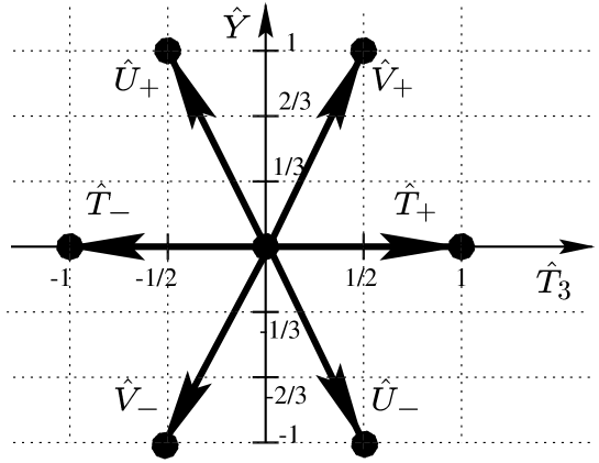
Figure 2: Action of the ladder operators on the $T_{3}$ – $Y$ plane

It can be seen, that the $su(3)$ algebra contains three $su(2)$ subalgebras symmetrically.

Generally, SU(3) multiplets are hexagon (truncated triangle) shaped (For a simple explanation see e. g. in Ref. [21]). Due to the difficult structure of Casimir operators (not detailed here), usually the dimensions of these polygons are used for indexing the states. The multiplet denoted by $(\lambda,\mu)$ has

$$\lambda=2T_{3},\ \mbox{at}\ Y=Y_{\mbox{\scriptsize{max}}}$$ (20)

$$\mu=2T_{3},\ Y=Y_{\mbox{\scriptsize{min}}}.$$ (21)

Due to the additional symmetry of interchanging of bosons however, only the multiplets $(n,0)$ can be realized, where $n$ denotes the total number of the photons. Some of the multiplets are visualized on the $T_{3}$ – $Y$ plane in Fig. 3.

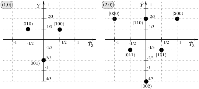
Figure 3: $SU(3)$-multiplets $(1,0)$ of one photon and $(2,0)$ of two photons visualized on the $\hat{T}_{3}$ – $\hat{Y}$ plane.

Having described the multiplets, now let us turn our attention to the description of the tritters alike that of beam splitters in Ref. [11]. The matrix $U$ describing the tritter in Eq. (13) can be decomposed into a generalized “Euler-angle” parameterization defined in Ref. [22]:

$$U(\alpha,\beta,\gamma,\theta,a,b,c,\phi)=e^{(i\hat{\lambda}_{3}\alpha)}e^{(i\hat{\lambda}_{2}\beta)}e^{(i\hat{\lambda}_{3}\gamma)}e^{(i\hat{\lambda}_{5}\theta)}e^{(i\hat{\lambda}_{3}a)}e^{(i\hat{\lambda}_{2}b)}e^{(i\hat{\lambda}_{3}c)}e^{(i\hat{\lambda}_{8}\phi)}.$$ (22)

This expression enables us to connect a standard parameterization of $SU(3)$ with the physical parameters of the actual realization of the tritter, such as transmittivity and reflectivity coefficients of the optical elements involved.

Similarly to the case of beam splitters, the action of a tritter may be described as follows: the input of the tritter can be described by the operators $\hat{F}_{1}\ldots\hat{F}_{8}$, which form a $su(3)$-algebra. From these operators, all the others described in Eqs. (4) can be expressed and used. The beam-splitter transformation $U$ defined in Eq. (13) turns these operators to operators $\hat{G}_{1}\ldots\hat{G}_{8}$ describing the output modes. The $\hat{G}$-s are formed from the $\hat{b}_{1},\hat{b}_{2},\hat{b}_{3}$ operators. The transformation $U$ is represented by the adjoint representation of $SU(3)$, which is a 8-parameter subgroup of the group $SO(8)$ of 8-dimensional rotations:

$$\hat{G}_{i}=U\hat{F}_{i}U^{\dagger}=\sum_{j=1}^{8}R_{ij}\hat{F}_{j},\quad R\in SO(8).$$ (23)

The explicit form of the $R$ matrices is given in Refs. [23, 24].

5 Conclusion

In this paper we have revisited $SU(2)$-description of beam splitters. We have presented an example of an optical setup in which only a few photon interfere, and have shown how the multiplet picture can help in understanding of the operation of such schemes.

We have outlined the $SU(3)$ description of optical tritters, describing bosonic realization of $SU(3)$ and showing the structure of the multiplets. The formalism suggested here maybe useful in applications of tritters, e.g. in few-photon interference experiments. The situation in case of tritters is similar to the case of the beam splitters, where 3 dimensional rotations occur, but unfortunately 8 dimensional rotations cannot be visualized.

References

- [1] K. Wódkiewicz and J. H. Eberly, “Coherent states and squeezed fluctuations, and the and ,” J. Opt. Soc. Am. B 2, pp. 458–466, 1985.
- [2] A. Luis and J. Perina, “ coherent states in parametric down-conversion,” Phys. Rev. A 53, pp. 1886–1893, 1996.
- [3] C. C. Gerry, “Remarks on the use of group theory in quantum optics,” Opt. Express 8, pp. 76–85, 2001.
- [4] M. G. Benedict and B. Molnár, “Algebraic construction of coherent states of the morse potential based on supersymmetric quantum mechanics,” Phys. Rev. A 60, pp. R1737–R1740, September 1999.
- [5] J. Janszky, A. Petak, C. Sibilia, M. Bertolotti, and P. Adam, “Optical Schrodinger-cat states in a directional coupler,” Quantum Semiclass. Opt. 7, pp. 145–152, 1995.
- [6] J. Fiurasek and J. Perina, “Substituting scheme for nonlinear couplers: A group approach,” Phys. Rev. A 62, No. 033808, 2000.
- [7] A. Karpati, P. Adam, J. Janszky, M. Bertolotti, and C. Sibilia, “Nonclassical light in complex optical systems,” J. Opt. B-Quantum Semicl. Opt. 2, pp. 133–139, 2000.
- [8] D. Bouwmeester, J.-W. Pan, K. Mattle, M. Eibl, H. Weinfurter, and A. Zeilinger, “Experimental quantum teleportation,” Nature 390, pp. 575–579, December 1997.
- [9] A. N. Boto, P. Kok, D. S. Abrams, S. L. Braunstein, C. P. Williams, and J. P. Dowling, “Quantum interferometric optical lithography: Exploiting entanglement to beat the diffraction limit,” Phys. Rev. Lett. 85, pp. 2733–2736, September 2000.
- [10] E. Knill, R. Laflamme, and G. J. Milburn, “A scheme for efficient quantum computation with linear optics,” Nature 409, pp. 46–52, 2001.
- [11] R. A. Campos, B. E. A. Saleh, and M. C. Teich, “Quantum-mechanical lossless beam splitter: symmetry and photon statistics,” Phys. Rev. A 40, pp. 1371–1384, August 1989.
- [12] D. T. Pegg, L. S. Phillips, and S. M. Barnett, “Optical state truncation by projection synthesis,” Phys. Rev. Lett. 81, pp. 1604–1606, August 1998.
- [13] S. M. Barnett and D. T. Pegg, “Optical state truncation,” Phys. Rev. A 60, pp. 4965–4973, December 1999.
- [14] M. Koniorczyk, Z. Kurucz, A. Gábris, and J. Janszky, “General optical state truncation and its teleportation,” Phys. Rev. A 62, No. 013802, June 2000.
- [15] A. Zucchetti, W. Vogel, and D. G. Welsch, “Quantum-state homodyne measurement with vacuum ports,” Phys. Rev. A 54, pp. 856–862, 1996.
- [16] Żukowski, A. Zeilinger, and M. A. Horne, “Realizible higher-dimensional two-particle entanglements via multiport beam splitters,” Phys. Rev. A 55, pp. 2564–2579, April 1997.
- [17] M. Żukowski and D. Kaszlikowski, “Greenberger-Horne-Zeilinger paradoxes with symmetric multiport beam splitters,” Phys. Rev. A 59, pp. 3200–3203, 1999.
- [18] J. A. Bergou, M. Hillery, and Y. Sun, “Non-unitary transformations in quantum mechanics: an optical realization,” J. Mod. Opt. 47(2), pp. 487 – 497, 2000.
- [19] L. C. Biedenharn and J. D. Louck, Angular momentum in quantum physics, Addison-Wesley, 1981.
- [20] M. Reck and A. Zeilinger, “Experimental realization of any discrete unitary operator,” Phys. Rev. Lett. 73, pp. 58–61, July 1994.
- [21] H. J. Lipkin, Lie groups for pedestrians, North-Holland Publishing CO., Amsterdam, 1965.
- [22] M. Byrd, “The geometry of ,” arXive e-print physics/9708015.
- [23] M. S. Byrd and E. C. G. Sudarshan, “ revisited,” arXive e-print physics/9803029.
- [24] M. Byrd and E. C. G. Sudarshan, “ revisited,” J. Phys. A-Math. Gen. 31, pp. 9255–9268, 1998.