Quantum homogenization

Abstract

We design a universal quantum homogenizer, which is a quantum machine that takes as an input a system qubit initially in the state $\rho$ and a set of $N$ reservoir qubits initially prepared in the same state $\xi$. In the homogenizer the system qubit sequentially interacts with the reservoir qubits via the partial swap transformation. The homogenizer realizes, in the limit sense, the transformation such that at the output each qubit is in an arbitratily small neighbourhood of the state $\xi$ irrespective of the initial states of the system and the reservoir qubits. This means that the system qubit undergoes an evolution that has a fixed point, which is the reservoir state $\xi$. We also study approximate homogenization when the reservoir is composed of a finite set of identically prepared qubits. The homogenizer allows us to understand various aspects of the dynamics of open systems interacting with environments in non-equilibrium states. In particular, the reversibility vs or irreversibility of the dynamics of the open system is directly linked to specific (classical) information about the order in which the reservoir qubits interacted with the system qubit. This aspect of the homogenizer leads to a model of a quantum safe with a classical combination.We analyze in detail how entanglement between the reservoir and the system is created during the process of quantum homogenization. We show that the information about the initial state of the system qubit is stored in the entanglement between the homogenized qubits.

PACS numbers: 03.65.Yz, 03.67.-a

I Introduction

When a system interacts with a reservoir which is in thermal equilibrium then after some time the system is thermalized - it relaxes towards the thermal equilibrium. This implies that the information about the original state of the system is (irreversibly) “lost” and its new state is determined exclusively by the parameters (temperature) of the reservoir. If the reservoir is composed of a large number, $N$, of physical objects of the same physical type as the system itself, then the thermalization process can be understood as homogenization: out of $N$ objects (the reservoir) prepared in the same thermal state and a single system in an arbitrary state, we obtain $N+1$ objects in the same thermal state. This intuitive picture is based on certain assumptions about the interaction between the system and the reservoir, about the physical nature of the reservoir itself and the concept of the thermal equilibrium. This picture is at the heart of the model of blackbody radiation, which triggered the birth of quantum theory in the seminal work of Planck. In addition, this same picture is very important in understanding many processes in quantum physics as well as the fundamental concept of the irreversibility [1, 2].

In this paper we present a rigorous analysis of the above picture within the framework of quantum information theory. Specifically, we will consider a system, $S$, represented by a single qubit initially prepared in the unknown state $\varrho_{S}^{(0)}$, and a reservoir, $R$, composed of $N$ qubits all prepared in the state $\xi$, which is arbitrary but same for all qubits. We will enumerate the qubits of the reservoir and denote the state of the $k$-th qubit as $\xi_{k}$ [3]. From the definition of the reservoir it follows that initially $\xi_{k}=\xi$ for all $k$, so the state of the reservoir is described by the density matrix $\xi^{\otimes N}$.

Let $U$ be a unitary operator representing the interaction between a system qubit and one of the reservoir qubits. In addition, let us assume that at each time step the system qubit interacts with just a single qubit from the reservoir (see Fig. 1). Moreover, the system qubit can interact with each of the reservoir qubits at most once. After the interaction with the $1$-st reservoir qubit the system is changed according to the following rule (which is a completely-positive map)

$$\varrho_{S}^{(1)}={\rm Tr}_{1}\left[U\varrho_{S}^{(0)}\otimes\xi_{1}U^{\dagger}\right].$$ (1)

FIG. 1.: The scenario of homogenization with just three reservoir qubits involved.

Let us repeat the interaction $N$ times, that is, via a sequence of interactions the system qubit interacts with $N$ reservoir qubits all prepared in the state $\xi$. The final state of the system is then described by the density operator

$$\varrho_{S}^{(N)} = {\rm Tr}_{R}\left[U_{N}\dots U_{1}\left(\varrho_{S}^{(0)}\otimes\xi^{\otimes N}\right)U_{1}^{\dagger}\dots U_{N}^{\dagger}\right]$$ (2)

where $U_{k}:=U\otimes(\bigotimes_{j\neq k}\openone_{j})$ describes the interaction between the $k$-th qubit of the reservoir and the system qubit. This model of homogenization is very similar to the collision model since the system becomes homogenized via a sequence of individual interactions with the reservoir qubits. The interactions are assumed to be localized in time (i.e., they act like ellastic collisions) [4].

Our aim is to investigate possible maps induced by the transformation (2) and describe the process of homogenization. Homogenization means that due to the interaction $U$ the states of the qubits in reservoir change only little while after $N$ interactions the system’s state become close to the initial state of the reservoir qubits. Formally,

$$\forall N\geq N_{\delta} \dots\dots D(\varrho_{S}^{(N)},\xi)\leq\delta\,;$$ (3)

$$\forall k,1\leq k\leq N \dots\dots D(\xi_{k}^{\prime},\xi)\leq\delta,$$ (4)

where $D(.,.)$ denotes some distance (e.g., a trace norm) between the states, $\delta>0$ is a small parameter which is chosen a priori to the determine the degree of the homogeneity and $\xi_{k}^{\prime}:={\rm Tr}_{S}[U\varrho_{S}^{(k-1)}\otimes\xi U^{\dagger}]$ is the state of the $k$-th reservoir qubit after the interaction with the system qubit.

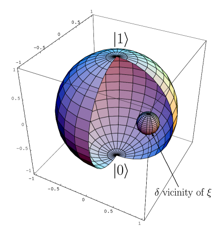
FIG. 2.: The $\delta$ neighborhood of the reservoir’s state $\xi$ inside the Bloch sphere. After $N$ interactions between the system and the reservoir the states of all reservoir qubits and the system qubit are contained within this $\delta$-sphere.

The conditions (3) and (4) can be represented using a geometrical picture. The Bloch sphere of unit radius is a representation of the state space of a spin-1/2 (qubit) system. The initial state $\rho$ of the system qubit and the reservoir state $\xi$ are represented by two (distinct) points of the Bloch sphere. We can image another sphere of the radius $\delta$ centered at the point representing the reservoir state $\xi$ (in what follows we will call this sphere the $\delta$-sphere). The task is to “shrink” the original Bloch sphere representing the (unknown) initial state space of the system qubit into the $\delta$-sphere. So we start with $N$ reservoir qubits in the state $\xi$ and the system qubit in an arbitrary state $\rho$ and we end up with $N+1$ qubits within the $\delta$-sphere centered at the point representing the original reservoir state $\xi$ (see Fig. 2).

We note that homogenization is closely related to thermalization. There are however two main differences: in thermalization, (i) the state $\xi$ of the reservoir qubits is not completely unknown, but is a thermal state, that is, a state diagonal in a given basis (interpreted as the basis of the eigenstates of a one-qubit Hamiltonian); and (ii) the number of qubits in the reservoir is considered to be infinite for any practical purpose. Thermalization is studied in Ref. [5].

Our paper is organized as follows: in Section II we show that quantum homogenization can be realized with the help of a partial swap operation. In Section III we show that the partial swap for qubits generates a contractive map on the system qubit with the fixed point being the initial state of the reservoir. This ensures the required convergence of the homogenization process [see Eqs. (3) and (4)]. The uniqueness of the partial-swap operation is proved in Section IV. In Section V we estimate the fidelity of the approximate homogenization map as a function of the number $N$ of reservoir qubits and the parameter $\delta$ (the precision of the homogenization), while in the Section VI we will analyze how the reservoir qubits become entangled as a consequence of their interaction with the system qubit. In the final Section VII of the paper we address possible applications of the homogenization map.

II Partial-swap operation

Let us start with the definition of the so-called swap operation $S$ acting on the Hilbert space of two qubits which is given by relation [6]

$$S|\psi\rangle\otimes|\phi\rangle=|\phi\rangle\otimes|\psi\rangle.$$ (5)

With this transformation

$$S\,\varrho^{(0)}\otimes\xi\,S^{\dagger}\,=\,\xi\otimes\varrho^{(0)}\;,$$ (6)

after just a single interaction, the state of the system $S$ is equal to the state $\xi$ of the reservoir qubit; and the interacting qubit from the reservoir is left in the initial state of system. This means the condition (3) is fulfilled, while the condition (4) is not — since recall that we want it to hold for all $\varrho^{(0)}$.

In order to fulfill both conditions (3) and (4) we have to find some unitary transformation which is “close” to the identity on the reservoir qubit, while it performs a partial swap operation, so that the system qubit at the output is closer to the reservoir state $\xi$ than before the interaction. The swap operator is Hermitian and therefore we can define the unitary partial swap operation

$$P(\eta)=\cos\eta\,\openone\,+\,i\,\sin\eta\,S$$ (7)

that serves our purposes. In what follows we denote $\sin\eta=s$ and $\cos\eta=c$.

In the process of homogenization, the system qubit interacts sequentially with one of the $N$ qubits of the reservoir through the transformation $P(\eta)$. After the each interaction, the system qubit becomes entangled with the qubit of the reservoir with which it interacted (for more details on the issue of entanglement see Sec. VI) The states of the system qubit and of the reservoir qubit are obtained by partial traces. Specifically, after the first interaction the system qubit is in the state described by the density operator

$$\varrho_{S}^{(1)}=c^{2}\varrho_{S}^{(0)}+s^{2}\xi+ics[\xi,\varrho_{S}^{(0)}],$$ (8)

while the first reservoir qubit is now in the state

$$\xi_{1}^{\prime}=s^{2}\varrho_{S}^{(0)}+c^{2}\xi+ics[\varrho_{S}^{(0)},\xi].$$ (9)

We can recursively apply the partial-swap transformation and after the interaction with the $n$-th reservoir qubit, we have

$$\varrho_{S}^{(n)}=c^{2}\varrho_{S}^{(n-1)}+s^{2}\xi+ics[\xi,\varrho_{S}^{(n-1)}]\,,$$ (10)

as the expression for the density operator of the system qubit, while the $n$-th reservoir qubit is in the state

$$\xi_{n}^{\prime}=s^{2}\varrho_{S}^{(n-1)}+c^{2}\xi+ics[\varrho_{S}^{(n-1)},\xi]\,.$$ (11)

Since we are interested only in those terms in expressions (10) and (11) that are proportional to the operator $\xi$ we can rewrite the above equations in the form

$$\varrho_{S}^{(n)}=s^{2}\sum_{k=0}^{n-1}c^{2k}\xi+\rho_{rest}^{(n)}=(1-c^{2n})\xi+\rho_{rest}^{(n)}\,,$$ (12)

and

$$\xi_{n}^{\prime}=s^{2}(1-c^{2(n-1)})\xi+\xi_{n,rest}\,.$$ (13)

In the next section, we are going to show that $\rho_{rest}^{(n)}$ converges monotonically to the null operator as $n\rightarrow\infty$. In this case, obviously $\varrho_{S}^{(n)}\rightarrow\xi$, so the condition (3) is fulfilled if the number of qubits $N$ is large enough. In addition, as $n$ increases, $\xi^{\prime}_{n}$ becomes more and more similar to $\xi$, since the commutator in (11) goes to zero; in other words,

$$D(\xi_{n}^{\prime},\xi)\leq D(\xi_{n-1}^{\prime},\xi)\,.$$ (14)

Therefore, condition (4) will be fulfilled for all $k$ if and only if it is fulfilled for $k=1$. This gives us a restriction on the parameter $\eta$ that enters the partial swap; this restriction will be studied in Section V.

III Homogenization is a contractive map

In this section we want to show that $\varrho^{(N)}_{S}\to\xi$ monotonically, for all parameters $\eta\neq 0$. This means, in particular, that condition (3) does not put any constraint on $\eta$. To show this convergence, we use the Banach theorem [7] that concerns the fixed point of a contractive transformation. Let $\cal S$ be a space with a distance function $D(\varrho,\xi)$, then the transformation $T$ is called contractive if it fulfills the inequality $D(T[\varrho],T[\xi])\leq kD(\varrho,\xi)$ with $0\leq k<1$ for all $\varrho,\xi\in\cal S$. A fixed point of the transformation $T$ is an element of $\cal S$ for which $T[\xi]=\xi$. The Banach theorem states that a contractive map has a unique fixed point [8], and that the iteration of the map converges to it, i.e. $T^{N}[\varrho]\to\xi$ for each $\varrho\in\cal S$. We note that contractive transformations within the context of quantum information processing have been recently discussed also in Ref. [9].

In our case $\cal S$ is the set of physical states, i.e. the set of all density matrices of a single qubit. The map, $T$, that we are considering is defined by $\varrho^{(0)}_{S}\to T[\varrho^{(0)}_{S}]=\varrho^{(1)}_{S}$. We must show that the map is contractive, and that $\xi$ is a fixed point of the map.

We begin by finding the super-operator induced by the transformation $U$ in the left-right form, i.e., as a linear operator acting on the space of trace-class operators ${\cal T}({\cal H})$ (see Ref. [10]). We choose the operators $\frac{1}{2}\openone,\sigma_{x},\sigma_{y},\sigma_{z}$ (where $\sigma_{n}$ are the Pauli matrices) as a basis for ${\cal T}({\cal H})$, where $\cal H$ represents the Hilbert space of a qubit. In this case an arbitrary density operator of a qubit can be written as

$$\varrho=\frac{1}{2}\openone+\vec{w}\cdot\vec{\sigma}$$ (15)

where $|\vec{w}|\leq 1/2$. We can write a state that is an element of ${\cal T}({\cal H})$ in a vector form, i.e. $\varrho=(1,w_{x},w_{y},w_{z})$. Let $\xi=\frac{1}{2}\openone+\vec{t}\cdot\vec{\sigma}=(1,t_{x},t_{y},t_{z})$ be the state of the qubit in the reservoir. After the first interaction $P$ with the first reservoir qubit the system qubit evolves according to Eq.(10) with $n=1$. This transformation can be described as

$$\varrho^{(0)}_{S}\to\varrho^{(1)}_{S} = s^{2}\xi+c^{2}\varrho^{(0)}_{S}+ics[\xi,\varrho^{(0)}_{S}]$$ (16)

$$= \frac{1}{2}\openone+(s^{2}\vec{t}+c^{2}\vec{w})\cdot\vec{\sigma}+ics[\vec{t}\cdot\vec{\sigma},\vec{w}\cdot\vec{\sigma}]$$ (17)

$$= \frac{1}{2}\openone+[s^{2}\vec{t}+c^{2}\vec{w}-2cs(\vec{t}\times\vec{w})]\cdot\vec{\sigma}$$ (18)

$$= \frac{1}{2}\openone+\vec{w}^{~{}\prime}\cdot\vec{\sigma},$$ (19)

where we used the identity $\sigma_{k}\sigma_{l}=\delta_{kl}\openone+i\varepsilon_{jkl}\sigma_{j}$, and

$$w^{\prime}_{j}=s^{2}t_{j}+(c^{2}\delta_{jl}-2cs\,\varepsilon_{jkl}t_{k})w_{l}\,,$$ (20)

with $j=x,y,z$. Now we can express the transformation $\varrho^{(0)}_{S}\to\varrho^{(1)}_{S}$ as

$$\left(\begin{array}[]{c}1\\ w_{x}^{\prime}\\ w_{y}^{\prime}\\ w_{z}^{\prime}\end{array}\right)=\left(\begin{array}[]{cccc}1&0&0&0\\ s^{2}t_{x}&c^{2}&2cst_{z}&-2cst_{y}\\ s^{2}t_{y}&-2cst_{z}&c^{2}&2cst_{x}\\ s^{2}t_{z}&2cst_{y}&-2cst_{x}&c^{2}\\ \end{array}\right)\left(\begin{array}[]{c}1\\ w_{x}\\ w_{y}\\ w_{z}\end{array}\right),$$ (21)

or more formally, as $\varrho^{(1)}_{S}=T\varrho^{(0)}_{S}$, where $T$ is the matrix representing the super-operator acting on the linear space ${\cal T}({\cal H})$. If we express the matrix $T$ as

$$T=\left(\begin{array}[]{cc}1&\vec{0}^{T}\\ s^{2}\vec{t}&{\bf T}\end{array}\right)\,,$$ (24)

then it is easy to check that in our case ${\bf T}\vec{t}=c^{2}\vec{t}$. This implies that the state $\xi$ is a fixed point of the map under consideration, i.e. $T\xi=\xi$. The system state after $n$-th iteration then reads

$$\varrho_{S}^{(n)} = \frac{1}{2}\openone+\left[\sum_{j=0}^{n-1}s^{2}{\bf T}^{j}\vec{t}+{\bf T}^{n}\vec{w}\right]\cdot\vec{\sigma}$$ (25)

$$= \frac{1}{2}\openone+\left[s^{2}\sum_{j=0}^{n-1}c^{2j}\vec{t}+{\bf T}^{n}\vec{w}\right]\cdot\vec{\sigma}\,$$ (26)

$$= \frac{1}{2}\openone+\left[(1-c^{2n})\,\vec{t}+{\bf T}^{n}\vec{w}\right]\cdot\vec{\sigma}\,,$$ (27)

where for the last equality we summed the geometric sum $\sum_{j=0}^{n-1}(c^{2})^{j}=(1-c^{2n})/(1-c^{2})$. Of course, $c^{2n}\to 0$ unless $c=\cos\eta=1$. Numerically one can check that ${\bf T}^{n}\to{\bf O}$, where ${\bf O}$ represents the zero operator. Thus $\varrho^{(n)}_{S}\to\xi$. In what follows we prove this convergence for all values of the parameter $\eta$.

To prove that the map $T$ is contractive, we must define a distance function on $\cal{S}$. Let us introduce the trace distance $D(\varrho,\omega)={\rm Tr}|\varrho-\omega|$ and the vectors $\omega=(1,v_{x},v_{y},v_{z})$ and $\vec{r}=\vec{w}-\vec{v}$. For a qubit we have

$$D(\varrho,\omega)={\rm Tr}|(\vec{w}-\vec{v})\cdot\vec{\sigma}|={\rm Tr}|\vec{r}\cdot\vec{\sigma}|\,=\,2|\vec{r}|$$ (28)

since the eigenvalues of the operator $\vec{r}\cdot\vec{\sigma}$ are given by $\lambda_{\pm}=\pm|\vec{r}|$. In order to find the contraction parameter $k$ for our transformation $T$ we proceed as follows. From the Eqs. (24) and (28) we obtain

$$D(T[\varrho],T[\omega])={\rm Tr}|\vec{r}^{~{}\prime}\cdot\vec{\sigma}|\,=\,2|\vec{r}^{~{}\prime}|,$$ (29)

where $\vec{r}^{~{}\prime}=\vec{w}^{~{}\prime}-\vec{v}^{~{}\prime}=s^{2}\vec{t}+{\bf T}\vec{w}-s^{2}\vec{t}-{\bf T}\vec{v}={\bf T}(\vec{w}-\vec{v})={\bf T}\vec{r}=c^{2}\vec{r}-2cs\vec{t}\times\vec{r}$. Since $|\vec{t}|^{2}\leq 1/4$ and $|\vec{r}^{~{}\prime}|^{2}=c^{4}|\vec{r}|^{2}+4c^{2}s^{2}|\vec{t}\times\vec{r}|^{2}=|\vec{r}|^{2}c^{2}(c^{2}+4s^{2}|\vec{t}|^{2}\sin^{2}\beta)$, where $\beta\leq\pi$ is the angle between the vectors $\vec{t}$ and $\vec{r}$, we find that the contraction coefficient $k=c$. This last equality is due to the fact that $|\vec{r}^{~{}\prime}|\leq|\vec{r}|c$. If $c=\cos\eta<1$ then the map $T$ is contractive and the convergence to the fixed point $\xi$ is assured.

IV Uniqueness of the partial-swap operation

In what follows we will discuss the question of the choice of the unitary transformation, ${U}$, that describes the interaction between a system from the reservoir and the initial system undergoing the homogenization process. If both the system and the reservoir state are the same, the interaction should not affect either qubit, and this should be true no matter what the state of the system and reservoir qubit are. This implies that the unitary operator must satisfy the following two conditions:

$${\rm Tr}_{1}\left({U}\rho\otimes\rho{U}^{\dagger}\right) = \rho\;,$$ (30)

$${\rm Tr}_{S}\left({U}\rho\otimes\rho{U}^{\dagger}\right) = \rho\;,$$ (31)

for any single-qubit state, $\rho$. Let us first discuss the case of pure states. If $\rho$ represents a pure state then the condition (30) says that ${U}\rho\otimes\rho{U}^{\dagger}=\rho\otimes\xi_{1}$ where $\xi_{1}$ needs to be determined. However from the second condition (31) it follows that ${U}\rho\otimes\rho{U}^{\dagger}=\xi_{2}\otimes\rho$ where $\xi_{2}$ is unknown. Putting the last two results together we obtain that

$${U}\rho\otimes\rho{U}^{\dagger}=\rho\otimes\rho\;,$$ (32)

for any $\rho$ representing a pure state. From here it follows that the unitary transformation ${U}$ acting on the joint Hilbert space ${\cal H}^{2}={\cal H}\otimes{\cal H}$ must be of the form

$${U}:|\psi\rangle\otimes|\psi\rangle\rightarrow e^{i\varphi}|\psi\rangle\otimes|\psi\rangle\;,$$ (33)

where the parameter $\varphi$ is independent of the state $|\psi\rangle$. Therefore, the action of the unitary transformation is fixed on the symmetric subspace of ${\cal H}^{2}$ up to a phase factor $e^{i\varphi}$. Neither of the two conditions (30) and (31) nor the condition (33) tell us anything about the action of the unitary transformation ${U}$ on the antisymmetric subspace of ${\cal H}^{2}$. This means that action of ${U}$ on the antisymmetric subspace is arbitrary. However, in the case of qubits the antisymmetric subspace is one dimensional, and we can proceed further. Because the antisymmetric subspace is one dimensional and invariant under the action of the unitary transformation ${U}$, we have

$${U}(|\psi\rangle|\psi^{\perp}\rangle-|\psi^{\perp}\rangle|\psi\rangle)=e^{i\theta}\left(|\psi\rangle|\psi^{\perp}\rangle-|\psi^{\perp}\rangle|\psi\rangle\right)\;,$$ (34)

where $\theta$ is a constant depending on ${U}$. Now the transformation ${U}$ is given by the equations (33) and (34) up to two constants $\varphi$ and $\theta$. What we would now like to show is that these conditions require that $U$ be a partial swap operator up to a global phase factor. This phase factor has no physical consequences. If we define the unitary operator $U^{\prime}$ to be

$${U}^{\prime}=\exp^{i(-\theta-\varphi)/2}{U}\;,$$

then equations (33) and (34) give us

$$|\psi\rangle|\psi\rangle \stackrel{{\scriptstyle U^{\prime}}}{{\rightarrow}} e^{i(\varphi-\theta)/2}|\psi\rangle|\psi\rangle$$

$$|\psi\rangle|\psi^{\perp}\rangle-|\psi^{\perp}\rangle|\psi\rangle) \stackrel{{\scriptstyle U^{\prime}}}{{\rightarrow}} e^{i(\theta-\varphi)/2}\left(|\psi\rangle|\psi^{\perp}\rangle-|\psi^{\perp}\rangle|\psi\rangle\right)\;.$$

Comparing these equations to Eq. (7), we see that $U^{\prime}$ is just the partial-swap operator with $\eta=(\varphi-\theta)/2$. We can, therefore, conclude that in the case of qubits, the partial swap is the only possible operator that satisfies the conditions of homogenization (30) and (31). The partial-swap uniquely determines yet another universal quantum machine [11]: the universal quantum homogenizer.

V Approximate homogenization

In what follows we will analyze homogenization not as the limit of the infinite number of interactions, but as an approximate process after a finite number of steps. Let us suppose that the parameter $\delta$ from Eqs. (3) and (4) is fixed. This parameter characterizes our approximation. We will use the partial-swap evolution for the description of the homogenization.

In the first step we give a condition on the parameter $\eta$ of the partial swap (7). For our map $T$, we have that $D(\varrho_{S}^{(N)},\xi)\leq D(\varrho_{S}^{(N-1)},\xi)\leq D(\varrho_{S}^{(0)},\xi)$. On the other hand from Eq. (14) we know that $D(\xi_{N}^{\prime},\xi)\leq D(\xi^{\prime}_{N-1},\xi)$. As we have discussed earlier, we can adjust the parameter $\eta$ so that the condition $D(\xi_{1}^{\prime},\xi)\leq\delta$ is fulfilled. Obviously, the distance $D(\xi_{1}^{\prime},\xi)$ depends on the initial state of the system, $\varrho_{S}^{(0)}$, and on $\eta$. Therefore we have to determine the maximum value of $\eta$, for which the distance is less than or equal to $\delta$, independent (the universality condition) of the initial states of the system and reservoir. For a qubit the maximum value of trace distance is achieved for $\vec{w}=-\vec{t}$, corresponding to the situation in which the states are pure and mutually orthogonal. The argument for this can be easily seen from a geometric representation of a qubit. In this case

$$D(\xi^{\prime}_{1},\xi)=2s^{2}{\rm Tr}|\vec{t}\cdot\vec{\sigma}|=2s^{2}$$ (35)

since for a pure state $|\vec{t}|=\frac{1}{2}$. From Eq. (35) we get the simple relation

$$\sin\eta\,\leq\,\sqrt{\delta/2}\;.$$ (36)

The second step is to determine the minimum number of interactions, $N$, that ensures for an arbitrary initial state of the system that the final state is in a sphere of radius $\delta$ around the reservoir state $\xi$. The worst case, i.e. when the number of necessary iterations is maximal, is intuitively the case when $D(\varrho_{S}^{(0)},\xi)$ is maximal. In section III we proved the convergence of the system state to $\xi$ for any $\eta\neq 0$. Therefore we are sure that such an $N$ exists. As was just discussed in the previous paragraph, the distance $D(\varrho_{S}^{(0)},\xi)$ is maximal, when the two states are pure and mutually orthogonal. Moreover, our transformation $T$ doesn’t change the commutation relation, which is initially equal to zero, i.e. $[\varrho_{S}^{(N)},\xi]=0$, for all $N$. Introducing $\vec{w}=-\vec{t}$ for the commuting states we obtain

$$\varrho_{S}^{(N)}=\frac{1}{2}\openone+(1-2c^{2N})\vec{t}\cdot\vec{\sigma}\,,$$ (37)

and for the distance we find

$$D(\varrho_{S}^{(N)},\xi)={\rm Tr}|(\vec{w}^{~{}\prime}-\vec{t})\cdot\vec{\sigma}|=2c^{2N}{\rm Tr}|\vec{t}\cdot\vec{\sigma}|\,.$$ (38)

This distance is maximal if we fix $N$ and maximize over all $\varrho_{S}^{(0)}$ and $\xi$. Again, since $|\vec{t}|=\frac{1}{2}$ for pure states, we obtain the distance $D(\varrho_{S}^{(N)},\xi)=2c^{2N}=2(\cos\eta)^{2N}$. If the parameters $\eta$ and $s$ in the experession (36) are such that $\sin\eta=\sqrt{\delta/2}$ then we can find the lower bound $N_{\delta}$ on the number of reservoir qubits which are necessary to achieve the homogenization with a required fidelity

$$N\,\geq N_{\delta}=\,\frac{\ln\delta/2}{\ln(1-\delta/2)}\,.$$ (39)

Both bounds on the parameters $\eta$ and $N$ are completely determined by the parameter $\delta$. After performing $N$ iterations, $N+1$ qubits are in states belonging to the $\delta$ neighborhood of the initial state of the reservoir, no matter what the states $\xi$ and $\varrho_{S}^{(0)}$ were.

We see that if we fix the number of reservoir’s qubits $N$, then the other two parameters are determined by the relations (39) and (36).

VI Entanglement via homogenization

In spite all the progress in the understanding of the nature of quantum entanglement there are still open questions that have to be answered. In particular, a problem which waits for a thorough illumination is the nature of multiparticle entanglement [13]. There are several aspects of quantum multiparticle correlations that have been investigated recently. One example is the investigation of intrinsic $N$-party entanglement (i.e, generalizations of the GHZ state [14]). Another is the realization that in contrast to classical correlations, entanglement cannot freely be shared among many objects.

Coffman et al. [15] have recently studied a set of three qubits, and have proved that the sum of the entanglement (measured in terms of the tangle) between the qubits $1$ and $2$ and the qubits $1$ and $3$ is less than or equal to the entanglement between qubit $1$ and the rest of the system, i.e. the subsystem $23$. Specifically, let us define the bi-partite concurrence [16] of a two-qubit system in the state $\varrho_{jk}$ to be:

$$C_{jk}\equiv C(\varrho_{jk}):=\max\{0,\lambda_{1}-\lambda_{2}-\lambda_{3}-\lambda_{4}\}$$ (40)

where the $\lambda_{i}$s are the square roots of the eigenvalues of the matrix $R=\varrho_{jk}(\sigma_{y}\otimes\sigma_{y})(\varrho_{jk})^{*}(\sigma_{y}\otimes\sigma_{y})$ listed indecreasing order. The tangle is equal to the square of the concurrence, i.e. $\tau_{jk}=[C_{jk}]^{2}$. Using this definition we can express the Coffman-Kundu-Wootters (CKW) [15] inequality as

$$C_{12}^{2}+C_{13}^{2}\leq C^{2}_{1,(23)}\,.$$ (41)

In the same paper they conjectured that a similar inequality might hold for an arbitrary number, $N$, of qubits prepared in a pure state. That is, one has

$$\sum_{k=1;k\neq j}^{N}C^{2}_{j,k}\leq C^{2}_{j,\overline{j}}\,,$$ (42)

where the sum in the left-hand-side is taken over all qubits except the qubit $j$, while $C^{2}_{j,\overline{j}}$ debotes the concurrence between the qubit $j$ and the rest of the system (denoted as $\overline{j}$).

Several interesting results in the investigation of various bounds on entanglement in multi-partite systems have been reported recently. In particular, Wootters [17] has considered an infinite collection of qubits arranged in an open line, such that every pair of nearest neighbors is entangled. In this translationally invariant entangled chain the maximum closest-neighbor (bi-partite) entanglement (measured in the concurrence) is bounded by the value $1/\sqrt{2}$ (it is not known whether this bound is achievable) [17]. Later Koashi et al. [18] considered a finite system of $N$ qubits in which each pair out of $N(N-1)/2$ possible pairs is entangled (the so-called web of entanglement). It has been proved that the maximum possible bi-partite concurrence in this case is equal to $2/N$. Dür [19] considered other possible inequalities associated with variously entangled qubits in multi-partite systems.

Within the context of our investigation it is very natural to ask, what is the nature of the entanglement created during the process of homogenization. In this section we will address several questions related to this issue. Firstly, we will study the bi-partite entanglement between the system qubit and the reservoir qubits, and then we will analyze entanglement between reservoir qubits which is induced by the interaction with the system qubit. We will show that CKW bounds are saturated, that is the $N+1$ qubit state created by a sequence of partial-swap operations in the homogenization process satisfies the inequality in Eq. (42) as an equality.

A Bipartite concurrence

Let us consider the concurrence $C^{(n)}_{jk}$ between the $j-$th and $k-$th qubits (irrespective whether these are reservoir or system qubits) after the $n-$th interaction, assuming that initially the system was in the state $\varrho$ and the reservoir qubits were in the state $\xi$. Without loss of generality we shall always assume that $j<k$. The value $j=0$ denotes the system qubit and $j=1,2,\dots,N$ denote the qubits of the reservoir.

The reduced density operator $\varrho^{(n)}_{jk}$ describing the two qubits under consideration is given by the expression

$$\varrho^{(n)}_{jk}={\rm Tr}_{\overline{j}\overline{k}}\left({\cal U}_{n}\dots{\cal U}_{1}[\varrho\otimes\xi^{\otimes N}]\right)\,,$$ (43)

with ${\cal U}_{l}[\sigma]=P_{l}\sigma P_{l}^{\dagger}$, where $P_{l}$ is the partial swap operation acting between the system qubit and the $l$-th qubit of the reservoir [see Eq.(7)]. The line over the indices in the trace formula denote the partial trace over all subsystems except the ones with the line over them.

Using the definition (40) of the concurrence, it is trivial to see that $C^{(n)}_{jk}=0$ for $j,k>n$, that is, the qubits which have not interacted yet are not entangled. On the other hand, a general expression for the concurrence is difficult to derive, so we concentrate our attention on a special case, when the reservoir is initially in a pure state $|\xi\rangle$ while the system qubit is in an arbitrary state $\varrho$.

Following the homogenization scenario the system qubit after $(k-1)$ interactions is in the state $\varrho_{0}^{(k-1)}$, that can be expressed in the basis $\{|\xi\rangle,|\xi^{\perp}\rangle\}$ as

$$\varrho_{0}^{(k-1)} = a_{k-1}|\xi\rangle\langle\xi|+(1-a_{k-1})|\xi^{\perp}\rangle\langle\xi^{\perp}|$$ (45)

$$+b_{k-1}|\xi\rangle\langle\xi^{\perp}|+b_{k-1}^{*}|\xi^{\perp}\rangle\langle\xi|.$$

After we apply the $k$-th partial swap operation between the system and the $k$-th reservoir qubit we find the bi-partite density operator in the matrix form (in the given basis)

$$\varrho_{0k}^{(k)}=\left(\begin{array}[]{cccc}a_{k-1}&cb_{k-1}&isb_{k-1}&0\\ b_{k-1}^{*}c&(1-a_{k-1})c^{2}&isc(1-a_{k-1})&0\\ -isb_{k-1}^{*}&-isc(1-a_{k-1})&s^{2}(1-a_{k-1})&0\\ 0&0&0&0\end{array}\right)$$ (46)

where $c=\cos\eta,s=\sin\eta$.

The matrix, $R$, constructed from $\varrho^{(k)}_{0k}$ has only one nonzero eigenvalue $4c^{2}s^{2}(1-a_{k-1})^{2}$. This implies for the concurrence

$$C_{0k}^{(k)}=2cs(1-a_{k-1}).$$ (47)

From Eq.(10) we find the recurrence formula for the parameters $a_{k}$

$$a_{k}=a_{k-1}c^{2}+s^{2}=1-c^{2k}(1-a_{0}),$$ (48)

from which we obtain

$$C_{0k}^{(k)}=2csc^{2(k-1)}(1-a_{0})$$ (49)

where $a_{0}:=\langle\xi|\varrho|\xi\rangle$, and $C_{0k}^{(k)}$ is the concurrence measuring the entanglement between the system qubit and $k-$th reservoir qubit just after their join interaction (i.e., it is supposed that the system qubit has interacted all together just $k$ times). We can conclude that the system qubit is entangled with $k$-th reservoir qubit. On the other hand we can ask whether this entanglement will persist after the system interacts later with other reservoir qubits. In order to make the discussion simpler we will study a particular case when initially the system is in the state $|1\rangle$ while the reservoir qubits are in the state $|0\rangle$. Nevertheless, prior to this task we study another aspect of multi-partite entanglement within the context of homogenization. Specifically, we will study how a given qubit is entangled with the rest of the system.

B One qubit vs rest of the system

In the case of pure multi-qubit states one can define a measure of the entanglement between a single qubit and the rest of the system [15] with the help of the determinant of the density operator of the specific qubit under consideration. In particular, let us begin the homogenization process with the system and the reservoir qubits initially in pure states. After $n$ partial swaps the $j$th qubit is in the state $\varrho_{j}^{(n)}={\rm Tr}_{\overline{j}}\left({\cal U}_{n}\dots{\cal U}_{1}[|\psi\rangle|\xi\rangle^{(\otimes N)}]\right)$. The degree of entanglement between the $j$th qubit and the rest of the system is given by the expression [15]

$$\tau^{(n)}_{j}\equiv\left[C_{j,\overline{j}}\right]^{2}:=4{\rm det}\varrho^{(n)}_{j}\,$$ (50)

where $\tau^{(n)}_{j}$ is the tangle, which is equal to the square of the corresponding concurrence.

Obviously, for the $j$th qubit of the reservoir, the tangle is zero until it interacts with the system qubit. After the interaction its value remains constant, irrespective of the further evolution of the system qubit during the homogenization process. This means that

$$\tau^{(n)}_{j}=\left\{\begin{array}[]{lcr}0&\ {\rm if}&\ n<j\leq N\\ 4{\rm det}\xi_{j}^{\prime}&\ {\rm if}&\ j\leq n\leq N\end{array}\right.$$ (51)

In order to justify the last equation we note that all measures of entanglement remain unchanged under local unitary transformations, and that all transformations ${\cal U}_{k}$ (except the $j$th one) are local with respect to the partition $j\oplus\overline{j}$ (where $\overline{j}$ denotes all qubits except $j$th).

The tangle between the system qubit and the reservoir is given by the expression

$$\tau^{(n)}_{0}=4{\rm det}\varrho_{0}^{(n)},$$ (52)

from which it follows that the shared entanglement between the system qubit and the whole reservoir depends on the total number of interactions $n$, unlike in the case (51) of the reservoir qubits.

C The case $|\psi\rangle_{0}=|1\rangle$ and $|\xi\rangle_{j}=|0\rangle$

In order to have a deeper insight into the problem of entanglement induced by the homogenization process, let us consider a specific initial state of the system and the reservoir: $|\psi\rangle_{0}=|0\rangle$ and $|\xi\rangle_{j}=|1\rangle$. In this case we find for the tangle between the system and the rest of the reservoir qubits after the $n$-th interaction the expression

$$\tau^{(n)}_{0}=4\det\varrho_{0}^{n}=4c^{2n}(1-c^{2n}),$$ (53)

since $\varrho_{0}^{(n)}=(1-c^{2n})|0\rangle\langle 0|+c^{2n}|1\rangle\langle 1|$ [cf. Eq. (12)]. It is clear from this expression that as $n\rightarrow\infty$ the degree of entanglement between the system and the reservoir is monotonically decreasing. On the other hand, the state of $j$-th qubit after the interaction with the system qubit is $\xi_{j}^{\prime}=s^{2}\varrho_{0}^{(j-1)}+c^{2}|0\rangle\langle 0|=(1-s^{2}c^{2(j-1)})|0\rangle\langle 0|+s^{2}c^{2(j-1)}|1\rangle\langle 1|$ [cf. Eq. (13)] from which it follows that

$$\tau^{(j)}_{j}=4s^{2}c^{2(j-1)}(1-s^{2}c^{2(j-1)})$$ (54)

In other words, after its interaction with the system qubit the $j$-th qubit is constantly entangled with the rest of the system. These simple examples illustrate the more general conclusions presented in the previous paragraph.

Let us turn our attention to the bipartite concurrences $C_{jk}^{(n)}$. With the given initial conditions, we easily find the state vector describing the whole system after $n$ interactions:

$$|\Psi\rangle=c^{n}|1\rangle_{0}\otimes|0\rangle^{\otimes N}+\sum_{l=1}^{n}|1\rangle_{l}\otimes|0\rangle^{\otimes N_{\overline{l}}}\left[isc^{l-1}(c+is)^{N-l}\right]\,.$$ (55)

We recall that $N$ is the total number of reservoir qubits, and that we have assumed that $j<k$. The state $|0\rangle^{\otimes N_{\overline{l}}}$ denotes all qubits except the qubit $l$ in the state $|0\rangle$. Tracing over the appropriate subsystems we find the density matrices for $j<n<k$,

$$\varrho_{jk}^{(n)} = \xi_{j}^{\prime}\otimes|0\rangle\langle 0|\,,$$ (56)

$$\varrho_{0k}^{(n)} = \varrho_{0}^{(j)}\otimes|0\rangle\langle 0|.$$ (57)

For $k\leq n$ we find

$$\varrho_{jk}^{(n)} = \left[c^{2n}+\sum_{l=1,l\neq k,j}^{n}s^{2}c^{2(k-1)}\right]|00\rangle\langle 00|$$ (61)

$$+s^{2}c^{2(k-1)}|01\rangle\langle 01|+s^{2}c^{2(j-1)}|10\rangle\langle 10|$$

$$+s^{2}c^{j+k-2}(c+is)^{k-j}|01\rangle\langle 10|$$

$$+s^{2}c^{j+k-2}(c-is)^{k-j}|10\rangle\langle 01|\,,$$

and

$$\varrho_{0k}^{(n)} = \sum^{n}_{l=1,l\neq k}s^{2}c^{2(l-1)}|00\rangle\langle 00|$$ (65)

$$+c^{2n}|10\rangle\langle 10|+s^{2}c^{2(k-1)}|01\rangle\langle 01|$$

$$+isc^{n+k-1}(c+is)^{n-k}|01\rangle\langle 10|$$

$$-isc^{n+k-1}(c-is)^{n-k}|10\rangle\langle 01|\,,$$

which determines the values of the concurrences. The corresponding eigenvalues of the matrices $R_{jk}^{(n)}$, constructed from the density matrices $\varrho_{jk}^{(n)}$ (in the case $n>k$), are

$${\rm eig}(R_{jk}^{(n)}) = \{4s^{4}c^{2(j+k-2)},0,0,0\}$$ (66)

$${\rm eig}(R_{0k}^{(n)}) = \{4s^{2}c^{2(n+k-1)},0,0,0\}.$$ (67)

The square roots of these eigenvalues are the $\lambda_{i}$s in Eq. (40). For the concurrences we find

$$C_{jk}^{(n)}=\left\{\begin{array}[]{lcl}0&\ {\rm for}&\ n<k\leq N\\ 2s^{2}c^{j+k-2}&\ {\rm for}&\ k\leq n\leq N\end{array}\right.\,,$$ (68)

$$C_{0k}^{(n)}=\left\{\begin{array}[]{lcl}0&\ {\rm for}&\ n<k\leq N\\ 2sc^{n+k-1}&\ {\rm for}&\ k\leq n\leq N\end{array}\right.\,.$$ (69)

We see that the concurrence between any two qubits of the reservoir is zero until both of them have interacted with the system qubit. Then the concurrence rises during the interaction to a new value and remains constant in the subsequent evolution. On the other hand the value of the entanglement between the system qubit and any qubit from the reservoir becomes nonzero after their joint interaction, but then it tends back to zero.

This means that the system qubit acts as a “mediator” of entanglement between the reservoir qubits which have never interacted directly. It is obvious that later the two reservoir qubits interact with the system qubit, the smaller the degree of their mutual entanglement. Nevertheless, this value is constant and does not depend on the subsequent evolution of the system qubit (i.e., it does not depend on the number of interactions $n$).

Once we have derived expressions for the bipartite concurrences, we can verify the CKW inequality (42), which in our notation takes the form

$$S_{j}(n):=\sum_{k=1}^{N}\left[C_{jk}^{(n)}\right]^{2}\leq\tau_{j}^{(n)}\equiv\left[C_{j,\overline{j}}^{(n)}\right]^{2}\,.$$ (70)

Firstly, let us consider the entanglement of the system qubit with the reservoir. Using Eq. (69) we can explicitly evaluate the expression for the left-hand-side of the inequality (70) and we can compare it with the expression (53) representing the right-hand-side of this inequality. We find that:

$$S_{0}(n)=\sum_{k=1}^{n}[C_{0k}^{(n)}]^{2}=4c^{2n}(1-c^{2n})=\tau^{(n)}_{0}\,,$$ (71)

which means that the bound on the bi-partite entanglement between the system and the reservoir qubits is saturated and the two sides are equal.

In fact, this property is also valid for the reservoir qubits. So, let us consider a qubit $j$ of the reservoir. In the case $n<j$ all the $C_{jk}^{(n)}$ vanish. That means $S_{j}(n)=0=\tau_{j}^{(n)}$. If $n\geq j$ then

$$S_{j}(n) = [C^{(n)}_{0j}]^{2}+\sum_{k=1}^{j-1}[C_{kj}^{(n)}]^{2}+\sum_{k=j+1}^{n}[C_{jk}^{(n)}]^{2}$$ (72)

$$= 4s^{2}c^{2(n+j-1)}+4s^{4}c^{2(j-2)}\left(\sum_{k=1}^{j-1}c^{2k}+\sum_{k=j+1}^{n}c^{2k}\right)$$ (73)

$$= 4s^{2}c^{2(n+j-1)}+4s^{4}c^{2(j-2)}(c^{2}-s^{2}c^{2j}-c^{2(n+1)})$$ (74)

$$= 4s^{2}c^{2(j-1)}(1-s^{2}c^{2(j-1)}).$$ (75)

In the calculation we used the equality

$$\sum_{k=1}^{j-1}c^{2k}+\sum_{k=j+1}^{n}c^{2k}=\sum_{k=0}^{n}c^{2k}-1-c^{2j}.$$ (76)

Comparing this result with Eq. (54) we obtain again the equality in Eq. (70)

$$S_{j}(n)=\tau_{j}^{(n)}=\left\{\begin{array}[]{lcl}0&\ {\rm for}&\ n\leq N\\ 4s^{2}c^{2(j-1)}\left[1-s^{2}c^{2(j-1)}\right]&\ {\rm for}&\ j\leq n\leq N\end{array}\right.$$ (77)

To understand in more detail the meaning of above expressions, let us consider the entanglement in the limit $N\to\infty$ of a very large number of qubits in the reservoir. We have to be careful with the definition of this limit. Let us first recall the definition of homogenization. We want to obtain homogenized qubits in states within some $\delta$-neighborhood of the reservoir’s state ($|0\rangle\langle 0|$ in our case). In Section V we showed that if we have a large number of qubits $N$, we can achieve an arbitrarily good homogenization, since in the bound (39) we can let $\delta\to 0$. In turn, the bound (36) means that $\delta\to 0$ is obtained for $s\to 0$. The behaviour of the expression $c^{2N}$ in this limit is as follows: Since $s\to 0$, then $c\to 1$, but still $c<1$, therefore $\lim_{N\to\infty}c^{2N}=0$, too. Now, looking at Eqs.(68),(69),(71) and (77), we see that in the limit $N\to\infty$ all the concurrencies vanish. Therefore, the shared entanglement between any pair of qubits is zero in this case, i.e. $\lim_{N\to\infty}C_{jk}^{(N)}=0$. Also the entanglement shared between a given qubit and rest of the homogenized system, expressed in terms of the function $S_{k}{(N)}$ is zero:

$$\lim_{N\to\infty}S_{k}{(N)}=0;\qquad k=0,1,\dots N$$ (78)

So, that’s how we define the limit $N\rightarrow\infty$: first, we assume that the system qubit has interacted with all the $N$ qubits in the reservoir, for $N$ finite; then, we let $N$ go to infinity, always assuming that we make the best possible homogenization according to the bounds of Section V.

As a first result, it is instructive to realize that in the limit $N\rightarrow\infty$ (when $\delta\rightarrow 0$) the functions $S_{0}(N)$ and $S_{j}(N)$ are such that

$$\lim_{N\rightarrow\infty}\frac{S_{0}(N)}{S_{k}(N)}=1,\qquad j=1,\dots N\,,$$ (79)

which means that the entanglement of the system qubit with the reservoir is the same as the entanglement of an arbitrary reservoir qubit to the rest of the homogenized system. This reflects the fact that not only states of individual qubits are the same but also the amount of entanglement between each of the qubits and the rest of the system are equal (see Fig. 3).

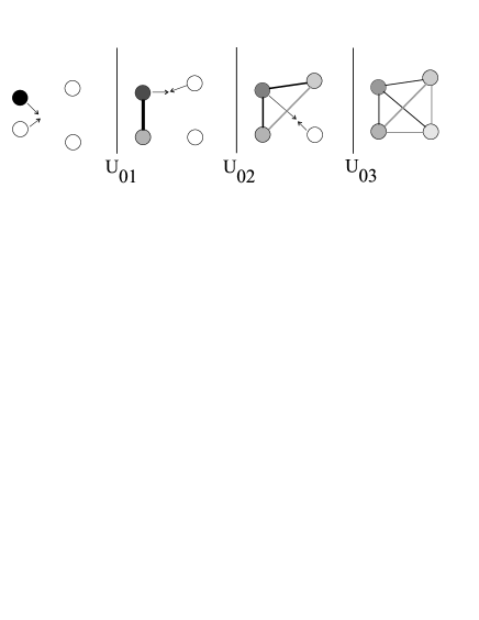
FIG. 3.: In this figure we schematically describe the process of entanglement between the system qubit and the reservoir qubits via the homogenization. The initial state of the whole system is shown in the left part of the figure: We have the system qubit denoted by the black circle, while the reservoir qubits are denoted as white circles. After the interaction ($U_{01}$) between the system and the first reservoir qubits a corresponding change of states (represented in different degrees of the grey color) and establishment of the entanglement (represented by the thick black line) is exhibited. After the interaction ($U_{02}$) with the second reservoir qubit, a three particle entangled state is created, with various degrees of bi-partite entanglement (represented by black and grey lines, where the grey line corresponds to the entanglement between reservoir qubits which have not interacted directly). In the right section of the figure we see the situation after the interaction ($U_{03}$) of the system qubit with the third reservoir qubit. All qubits are now entangled, black lines describe the entanglement between the system and the reservoir qubits which is established due to the direct interaction, while grey lines correspond to the entanglement between reservoir qubits induced by the interaction with the system qubit.

In spite of the fact that the pairwise entanglement between qubits in the limit $N\rightarrow\infty$ tends to zero, the information about the initial state of the system qubit is distributed among the homogenized qubits. Thus we have infinitely many infinitely small correlations between qubits and it seems that the required information is lost. However, as $N$ goes to infinity we have infinitely many qubits and the information redistributed among them has to be vanishingly small. If we sum up all the mutual concurrences between all qubits we obtain a finite value

$$\lim_{N\to\infty}\sum_{j<k}^{N}[C^{(N)}_{jk}]^{2}=\lim_{N\to\infty}\frac{1}{2}\sum_{j=0}^{N}S_{j}(N)=2.\,,$$ (80)

This supports our argument that the information about the initial state of the system is “hiden” in mutual correlations between qubits of the homogenized system. In the concluding section of the paper we will study how this information can be recovered.

To clarify the meaning of Eq. (80), we recall the recent results of Koashi et al. [18]. These authors have considered a system of $N$ qubits composing the web of entanglement. That is, each of $N(N-1)/2$ possible pairs of qubits is entangled, while the degree of entanglement is equal for all pairs. It has been shown that the maximal degree of pairwise entanglement in the web of entanglement is given by $C_{jk}^{(N)}=2/N$, that is the maximum tangle is $\tau=4/N^{2}$. Given that there are $N(N-1)/2$ possible pairs we find that the total value of the pairwise tangle is

$$\lim_{N\rightarrow\infty}\frac{N(N-1)}{2}\frac{4}{N^{2}}=2\,,$$ (81)

which is the same value as found in the homogenized system under consideration.

VII Conclusions and discussion:
Applications of homogenization

In this paper we have shown that one can choose a unitary transformation that exchanges information between a system qubit and a qubit from a reservoir, which, when applied sequentially to the system and each qubit in the reservoir, will generate an evolution that has the resevoir state as a fixed point. In fact, the state of the system qubit and those of the reservoir qubits become the same. Moreover, this unitary transformation, which we call the partial swap operation, is the only transformation, which is independent of the initial states of the system and the reservoir qubits, that will accomplish this.

This result is interesting per se since it allows us to understand in greater detail the dynamics of open systems [2]. It is also a nontrivial fact that the partial swap operation applied to the system qubit and a set of reservoir qubits allows us to realize an arbitrary contractive map of the system qubit [12].

On the other hand the results presented in the paper can be used in the context of quantum information processing. Specifically, quantum homogenization can be utilized for quantum cloning and in a protocol realizing a quantum safe with a classical combination.

A Quantum cloning

It is well known that unknown quantum states cannot be copied perfectly. Specifically, Wootters and Zurek[20] have presented a very simple proof that a perfect cloning transformation for unknown quantum states is impossible. The ideal quantum cloning scenario would look as follows: The quantum cloner is initially prepared in a state $|S\rangle$ which does not depend on the unknown state $|\psi\rangle$ of the input qubit which is going to be cloned. In addition, a qubit onto which the information is going to be copied is available. This particle is prepared in a known state denoted as $|0\rangle$. The perfect copying transformation ${\cal C}$ should be of the form

$$|\psi\rangle|0\rangle|S\rangle{\stackrel{{\scriptstyle\cal C}}{{\longrightarrow}}}|\psi\rangle|\psi\rangle|S^{\prime}\rangle$$ (82)

From the linearity of quantum mechanics it follows that the cloning transformation (82) is not possible.

Even though ideal cloning, i.e., the transformation (82), is prohibited by the laws of quantum mechanics for an arbitrary (unknown) state $|\psi\rangle$, it has been shown that it still possible to design quantum cloners which operate reasonably well [21]. These quantum cloners have been specified by the following conditions:

(i) The state of the original system and its quantum copy at the output of the quantum cloner, described by density operators $\hat{\rho}^{(out)}_{1}$ and $\hat{\rho}^{(out)}_{2}$, respectively, are identical, i.e.,

$$\hat{\rho}^{(out)}_{1}=\hat{\rho}^{(out)}_{2}.$$ (83)

(ii) If no a priori information about the in-state of the original system is available, then it is reasonable to require that all pure states should be copied equally well. One way to implement this assumption is to design a quantum copier such that the distances between density operators of each system at the output $\hat{\rho}^{(out)}_{j}$ (where $j=1,2$) and the ideal density operator $\hat{\rho}^{(id)}_{j}$ which describes the in-state of the original mode are input state independent.

(iii) Finally, it is also required that the copies are as close as possible to the ideal output state, which is, of course, just the input state. This means that the quantum copying transformation has to minimize the distance between the output state $\hat{\rho}_{j}^{(out)}$ of the copied qubit and the ideal state $\hat{\rho}_{j}^{(id)}$.

It has been shown by various authors that quantum cloners satisfying the above conditions do exist [21, 22]. Recently, experimental realizations of these quantum machines have been reported as well [23, 24]

However, this is not the only approach to quantum cloning; one can formulate the problem from a slightly different perspective using the ideas of quantum homogenization. First, one can lift the condition (83) that the qubits at the output are in the same state, that is, it can be assumed that the qubits at the output are in the states which are similar, but not identical. The second condition which might be lifted is that the “blank” qubit is initially in the known state $|0\rangle$. We can instead assume that both the input state of the original and that of the “blank” are unknown. If this point of view is adopted then the quantum homogenization as characterized by the conditions (3) and (4) can be successfully used for approximate cloning. Specifically, in this scenario the reservoir qubits play the role of originals, that is, it is the state $\xi$ we want to copy, while the system, which is supposed to be homogenized, (this system is initially in an unknown state $\varrho_{S}^{(0)}$) plays the role of the “blank” system onto which the information is going to be copied. From the description of quantum homogenization we see that quantum cloning in this context is a process in which we start with $N$ reservoir qubits, all in the same state $\xi$, and we end up with $N+1$ qubits in states which are very close (how close depends on the value of $N$) to the state $\xi$, so we have performed a version of $N\rightarrow N+1$ cloning on the reservoir state.

B Quantum safe with a classical combination

After the system qubit is homogenizaed it is in the same state as the reservoir qubits, so we can ask: What happened to the information encoded in the initial state of the system qubit? Is it irreversibly lost? Certainly not, because we considered only unitary transformations, and that means that the information encoded in the initial state of the system qubit is not lost but it is transferred into quantum correlations between all of the qubits. The parameters characterizing the state of the system are transformed into parameters determining the entanglement shared among the system and reservoir qubits. One question is whether the initial state of the system qubit can be recovered.

The process of homogenization is described by a sequence of unitary operations. Consequently, it can be reversed: That is the homogenized system can be “unwound” and the original state of the system $\varrho_{S}^{(0)}$ and the reservoir $\xi$ can be recovered. Perfect unwinding can be performed only when the $N+1$ qubits of the output state interact, via the inverse of the original partial-swap operation, in the “correct” order. The system particle must be identified from among the $N+1$ output qubits, and it and the reservoir particles must interact in the reverse of the order in which they originally interacted. Therefore, in order to unwind the homogenized system, the classical information about the ordering of the particles is vital. Obviously, if there are at the output $N+1$ particles, then there exists $(N+1)!$ permutations of possible orderings, only one of which will reverse the original process. The probability to choose the system particle, which is in the state $\varrho_{S}^{(N)}$, correctly is $1/(N+1)$. Even when this particle is chosen succesfully, then there are still $N!$ different possibilities in choosing the sequence of interactions with the reservoir qubits. If one has no knowledge about the output particles, the probability of successfully unwinding the homogenization transformation is $1/(N+1)!$. As we shall see, if at the beginning of the unwinding process the reservoir particle is chosen incorrectly then the whole process leads to a completely wrong result.

Therefore we can consider the quantum homogenization as a process that generates a combination to a quantum safe. The combination is the sequence in which the reservoir particles interact with the system particles, and the object in the safe is the initial state of the system particle. The combination consists of classical information, and the object in the safe consists of quantum information. The security here is given by the homogeneity of the final ensemble; it is difficult to distinguish among the particles by measuring them. The unwinding process can be performed reliably only when the combination is available. An important aspect of this scheme is that if one has tried one possible unwinding of the state, and measured the result to gain some information about it, it is not possible at that point to try to unwind it in a different way. That is, the nature of quantum mechanical measurement prevents repeated unwinding procedures on the same homogenized set of particles.

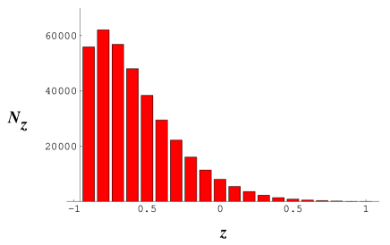
FIG. 4.: The result of the unwinding process with a trial-and-error strategy, when the system qubit is correctly chosen from a set of 10 homogenized particles. We plot a histogram representing number of reconstructed states of the system qubit with $s$ falling into the bin with $z=z_{n}\pm 0.05$. There are altogether $9!$ sequences we have checked and just one results in a correct reversal of the homogenization process.

To illustrate the above protocol let us assume that we begin with the system qubit in the state $|1\rangle$ and nine reservoir qubits in the $|0\rangle$. After quantum homogenization we try, randomly, to unwind the process. Let us assume that we are lucky and we have chosen the first qubit in the unwinding process correctly, that is, it is the original system qubit. Even with this good start, we have to find the rest of the combination, the proper sequence of the reservoir qubits, in order to completely “open” the quantum safe. Here we adopt a trial-and-error strategy, and we test all possible permutations of the reservoir qubits. Obviously, in this case just one sequence is correct, i.e. will result in opening the quantum safe and recovering the system state. All $9\,!=362880$ possible permutations of the reservoir qubits which were tested. Since we have chosen the states of the system and the reservoir qubits to be two orthogonal basis states of a single qubit, we can parameterize the reconstructed system state with just a single parameter $s$, i.e. $\rho_{unwound}=\frac{1}{2}(\openone+z\cdot\sigma_{z})=\frac{1+z}{2}|0\rangle\langle 0|+\frac{1-z}{2}|1\rangle\langle 1|$, such that $-1\leq z\leq 1$. In Fig.  4 we plot the histogram representing the number $N_{s}$ of reconstructed states of the system qubit with $s$ falling into the bin with $z=z_{n}\pm 0.05$. We see that a randomly chosen combination will not open the quantum safe. In fact, most of the reconstructed states are within the interval $-1\leq z\leq 0$, i.e. between the reservoir state and the completely random state.

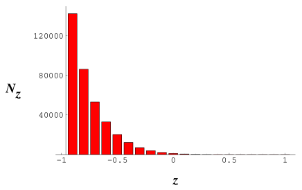
FIG. 5.: The result of the unwinding process with a trial-and-error strategy, when the system qubit is chosen incorrectly from a set of 10 homogenized particles. In the figure we represent results of $9\cdot 9!$ random unwindings. None of these sequences lead to the correct reversal of the original homogenization. We plot the histogram representing number of reconstructed states of the system qubit with $s$ falling into the bin with $z=z_{n}\pm 0.05$.

Let us now consider what happens when we choose the wrong qubit as the system qubit, i.e. what we have chosed as the system qubit was, in fact, one of the original reservoir qubits. As can be checked explicitly, in this case there is no way to correctly unwind the homogenization process. Obviously, with no prior knowledge, the probability to chose an incorrect system qubit from a set of $N+1$ homogenized qubits is $N$ time larger than the probability to chose the system qubit correctly. In addition, there are $N\cdot N!$ different sequences for the unwinding procedure in this case and none of them results in the initial state. In Fig. 5 we plot the results of these unwinding procedures for the same choice of the initial states as in the previous case.

We can conclude that the process of quantum homogenization can be unwound (i.e. reversed) if and only if classical information about the order of reservoir qubits is available. If this information is discarded, the process becomes irreversible even though the overall dynamics is unitary. This irreversibility can be used to protect quantum information. A detailed analysis of the security of the protocol we have proposed to do this remains to be done, but the example we have treated numerically strongly suggests that quantum information protected in this way is very secure.

- [1] A.Peres, Quantum Theory: Concepts and Methods (Kluwer, Dortrecht, 1993).
- [2] E.B. Davies, Quantum Theory of Open Systems (Academic, London, 1976).
- [3] We implicitely assume that the reservoir qubits are distinguishable. The validity of this assumption depends on the physical realization of the qubit. For instance, if the qubits are nuclear spins — or more generally, if each qubit is a degree of freedom of a given atom — the assumption is valid, since atoms are distinguishable from one another under normal conditions.
- [4] R. Alicki, K. Lendi, Quantum Dynamical Semigroups and Applications, Lecture Notes in Physics (Springer-Verlag, Berlin, 1987).
- [5] V. Scarani, M. Ziman, P. Štelmachovič, N. Gisin, and V. Bužek, quant-ph/0110088 (2001).
- [6] See for example: M. A. Nielsen and I. L. Chuang, Quantum Computation and Quantum Information (Cambridge University Press, Cambridge, 2000).
- [7] M. Reed and B. Simon, Methods of Modern Mathematical Physics I: Functional Analysis (Academic Press, San Diego, 1980)
- [8] This is very easy to see: suppose that and are two fixed points: then they must satisfy for a given . This is impossible unless .
- [9] M.Raginski, quant-ph/0105141 (2001).
- [10] M. B. Ruskai, S. Szarek, E. Werner, quant-ph/0101003 (2001).
- [11] G. Alber, T. Beth, M. Horodecki, P. Horodecki, R. Horodecki, M. Rötteler, W. Weinfurter, R. Werner, and A. Zeilinger, Quantum Information: An Introduction to Basic Theoretical Concepts and Experiments Springer Tracts in Modern Physics vol. 173 (Springer Verlag, Berlin, 2001).
- [12] J. Preskill, Lecture Notes on Quantum Computation, http://www.theory.caltech.edu/people/preskill/ph229/ #lecture.
- [13] A. V. Thapliyal, Phys. Rev. A 59, 3336 (1999); J. Kempe, Phys. Rev. A 60, 910 (1999).
- [14] D. M. Greenberger, et al., Am. J. Phys. 58, 1131 (1990).
- [15] V. Coffman, J. Kundu, W. K.Wootters, Phys.Rev. A 61, 052306 (2000).
- [16] S. Hill and W. K. Wootters, Phys. Rev. Lett. 78, 5022 (1997); W. K. Wootters, Phys. Rev. Lett. 80, 2245 (1998).
- [17] W. K. Wootters, quant-ph/0001114 (2000).
- [18] M. Koashi, V. Bužek, and N. Imoto, Phys. Rev. A 62, 050302(R) (2000).
- [19] W. Dür, Phys. Rev. A 63, 020303 (R) (2001).
- [20] W.K. Wootters and W.H. Zurek, Nature (London) 299, 802 (1982).
- [21] V. Bužek and M. Hillery, Phys. Rev. A 54, 1844 (1996)
- [22] N. Gisin and S. Massar, Phys. Rev. Lett. 79, 2153 (1997); D. Bruß, D. Vincenzo, A. Ekert, C. Fuchs, C. Macchiavello, and J. Smolin, Phys. Rev. A 57, 2368 (1998); R. Werner, Phys. Rev. A 58, 1827 (1998).
- [23] F.DeMartini and V. Musssi, Fort. der Physik 48, 413 (2000); F. DeMartini, V. Mussi, and F. Bovino, Opt. Commun. 179, 581 (2000).
- [24] Y.-F. Huang, W.-L. Li, Ch.-F. Li, Y.-S. Zhang, Y.-K. Jiang, and G.-C. Guo, Phys. Rev.. A 64, 012315 (2001).