Contents

toc

Chapter 1

QUANTUM-OPTICAL STATES IN
FINITE-DIMENSIONAL HILBERT SPACE.
II. STATE GENERATION

WIESŁAW LEOŃSKI

Nonlinear Optics Division, Institute of Physics, Adam Mickiewicz University, Poznań, Poland

ADAM MIRANOWICZ

CREST Research Team for Interacting Carrier Electronics, School of Advanced Sciences, The Graduate University for Advanced Studies (SOKEN), Hayama, Kanagawa, Japan and Nonlinear Optics Division, Institute of Physics,
Adam Mickiewicz University, Poznań, Poland

    I.  Introduction

As it was mentioned in the first part of this study [1], the finite-dimensional (FD) quantum-optical states have been a subject of numerous papers. For instance, various kinds of FD coherent states [2]–[6], FD Schrödinger cats [5, 6, 7], FD displaced number states [5], FD phase states [8], FD squeezed states [9, 10] were studied by many authors. In this chapter we concentrate on some schemes of generation of the FD quantum-optical states. These states can be produced as a finite superposition of $n$-photon Fock states. As a consequence, the problem of generation of FD states can be reduced to the choice of the mechanism of $n$-photon Fock state generation. For instance, Fock states can be achieved in the systems with externally driven cavity filled with the Kerr media [11]–[13]. Moreover, they can be produced in the cavities using micromaser trapped states [14]. Another way to obtain Fock states is that proposed by D’Ariano et. al. [15] based on the optical Fock-state synthesizer, in which the conditional measurements have been performed for the interferometer containing Kerr medium. The cavities with moving mirror [16] can also be utilized for the FD state generation. Recently, several schemes for the optical-state truncation (quantum scissors), by which FD quantum-optical states can be produced via teleportation, have been analyzed [17, 18]. Various other methods for preparation of Fock states [19] and their arbitrary superpositions [20] have been developed (see also Ref. [21]).

However, we shall concentrate here on the generation methods in which we are able to get directly the FD quantum state desired. Namely, we shall describe the models involving quantum nonlinear oscillator driven by an external field [11, 12, 13, 22]. For this class of systems we are able to get the quantum states that are very close for instance, to the FD coherent states [2, 3] or to the FD squeezed vacuum [10].

   II.  FD coherent states generated by nonlinear oscillator systems

This section is devoted to the method of generation of the FD coherent states making a class of states defined in FD Hilbert space. We shall concentrate on the states proposed by Bužek et al. [2] and further discussed by Miranowicz et al. [3, 23], where both the Glauber displacement operator and the states are defined in the FD Hilbert space [1]. The method of generation discussed here is based on the quantum systems containing a Kerr medium represented by nonlinear oscillator. It was introduced in Ref. [12] as a way of generating one-photon Fock states and was further adapted for the FD coherent-state generation [24]. The model discussed here represents a quantum nonlinear oscillator that interacts with an external field. Systems of this kind can be a source of various quantum states. For example, quantum nonlinear evolution can lead to generation of squeezed states [25], minimum uncertainty states [26], $n$-photon Fock states [11, 12, 13, 22], displaced Kerr states [27], macroscopically distinguishable superpositions of two states (Schrödinger cats) [28, 29] or higher number of states (Schrödinger kittens) [30]. Of course, the problem of practical realization of the system arises. At this point one should emphasize that the most commonly proposed practical realization is that in which a nonlinear medium is located inside one arm of the Mach–Zehnder interferometer [26]. However, models comprising a quantum nonlinear oscillator can be achieved in various ways. For instance, systems comprising trapped ions [31], trapped atoms [32] or cavities with moving mirror [16] can be utilized to generate states of our interest.

A.   Two-dimensional coherent states

Let us start the discussion of practical possibilities of the FD coherent-state generation from the simplest case, where only superpositions of vacuum and single-photon state are involved (the Hilbert space discussed is reduced to two dimensions). We consider the system governed by the following Hamiltonian defined in the interaction picture (in units of $\hbar=1$) to be

$$\hat{H}(t)=\frac{\chi}{2}({\hat{a}}^{\dagger})^{2}\hat{a}^{2}+\epsilon({\hat{a}}^{\dagger}+\hat{a})f(t)$$ (1.1)

where $\chi$ denotes the nonlinearity constant, which can be related to the third-order susceptibility of the Kerr medium; $\epsilon$ is the strength of the interaction with the external field, and $\hat{a}^{\dagger}$ and $\hat{a}$ are bosonic creation and annihilation operators, respectively. Moreover, using function $f(t)$ we are able to define the shape of the envelope of external field. For simplicity, we shall assume that the excitation is of the constant amplitude and hence, we put $f(t)=1$. Obviously, one should keep in mind that models discussed here concern a real physical situation (although they naturally involve certain limitation) and all operators, appearing in Eq. (1.1), are defined in the infinite-dimensional Hilbert space.

Let us express the wavefunction for our system in the Fock basis as

$$\left|\psi(t)\right>=\sum^{\infty}_{n=0}C_{n}(t)\left|n\right>$$ (1.2)

where the complex probability amplitude $C_{n}(t)$ corresponds to the $n$th Fock state $\left|j\right>$ and determines its time evolution. This wavefunction obeys the following Schrödinger equation

$$i\frac{d}{dt}\left|\psi(t)\right>=\left(\frac{\chi}{2}({\hat{a}}^{\dagger})^{2}\hat{a}^{2}+\epsilon({\hat{a}}^{\dagger}+\hat{a})\right)\left|\psi(t)\right>$$ (1.3)

for the Hamiltonian (1.1). Applying the standard procedure to our wavefunction (1.2) and Hamiltonian (1.1), we obtain a set of equations for the probability amplitudes $C_{n}(t)$. They are of the form

$$i\frac{d}{dt}C_{n}(t)=\frac{\chi}{2}n(n-1)C_{n}(t)+\epsilon\left[\sqrt{n}C_{n-1}(t)+\sqrt{n+1}C_{n+1}(t)\right]$$ (1.4)

where $n$ corresponds to the $n$-photon Fock state. Obviously, one should keep in mind that we deal with the infinite-dimensional Hilbert space and so the set of equations for $C_{n}(t)$, given by (1.4), is infinite too. However, our aim here is to show that under special conditions our system behaves as one defined in the FD Hilbert space. The first step is to assume that the external excitation is weak ($\epsilon\ll\chi$). As a consequence, we assume a perturbative approach. Moreover, and this is the main point of our considerations, the part of Hamiltonian (1.1) corresponding to the nonlinear evolution of the system

$$\hat{H}_{\mathrm{N}L}=\frac{\chi}{2}({\hat{a}}^{\dagger})^{2}\hat{a}^{2}$$ (1.5)

produces degenerate states corresponding to $n=0$ and $n=1$. As we take into account not only the first part of Hamiltonian (1.1) but also the second part, we see that a resonance arises between the interaction described by the latter and the degenerate states generated by $\hat{H}_{\mathrm{N}L}$. This resonance and the weak interaction lead to a situation when the system dynamics becomes of the closed form and cuts some subspace of states out of all the $n$-photon Fock states. As a consequence, assuming that the dynamics of the physical process starts from vacuum $\left|0\right>$, the evolution of the system is restricted to the states $\left|0\right>$ and $\left|1\right>$ solely. This situation resembles in some sense the problem of two degenerate atomic levels coupled by a zero-frequency field, where this resonant coupling selects, from the whole set of atomic levels, only those of them that lead to a closed system dynamics. For the case discussed here our system evolution corresponds to the two-level atom problem, where the interaction with remaining atomic states can be treated as a negligible perturbation [34]. Obviously, one should note that the character of the resonances commonly discussed in various papers, where the cavity field and the difference between the energies of the atomic levels (or cavity frequencies) have identical values, is different than that of those discussed here.

Thus, we write following equations of motion

$$i\frac{d}{dt}C_{0}(t) = \epsilon C_{1}(t)$$

$$i\frac{d}{dt}C_{1}(t) = \epsilon\left[C_{0}(t)+\sqrt{2}C_{2}(t)\right]$$ (1.6)

$$i\frac{d}{dt}C_{2}(t) = \chi C_{2}(t)+\epsilon\left[\sqrt{2}C_{1}(t)+\sqrt{3}C_{3}(t)\right]$$

$$\vdots$$

for the probability amplitudes corresponding to the system discussed here. Since we have assumed $\epsilon\ll\chi$, the Eqs. (1) indicate that the amplitude $C_{n}(t)$ rapidly oscillates in comparison with the amplitudes $C_{N}(t)$ if $n>{N}$. Hence, analogously to the description of driven atomic systems within the rotating wave approximation (RWA) [34], we neglect the influence of the probability amplitudes $C_{n}(t)$ for $n\geq 2$. Therefore, the dynamics of our system can be described by the following set of two equations

$$i\frac{d}{dt}C_{0}(t) = \epsilon C_{1}(t)$$

$$i\frac{d}{dt}C_{1}(t) = \epsilon C_{0}(t)$$ (1.7)

and their solution

$$C_{0}(t) = i\cos(\epsilon t)$$

$$C_{1}(t) = \sin(\epsilon t)$$ (1.8)

where we have assumed that the system starts its evolution from vacuum $\left|0\right>$. Clearly, this result resembles that for a two-level atom in an external field [34] and the dynamics of the system exhibits well-known oscillatory behavior. This result is identical to that derived for the simplest case (i.e., for $N=s+1=2$) of the FD generalized coherent states discussed by us in the first part of this work [1]. Of course, one should keep in mind that the set of Eqs. (1) gives zero-order solutions in perturbative treatment. As a consequence, the FD coherent states can be produced by the system discussed within the error following from this approximation.

The preceding result concerns the situation where the external excitation is characterized by a constant envelope: $f(t)=1$. For the general case, the solution can be obtained easily, applying the same procedure as for a resonantly driven two-level atom [34]. Then, the general solution can be expressed as

$$C_{0}(t) = i\cos\Theta(t)$$

$$C_{1}(t) = \sin\Theta(t)$$ (1.9)

where the symbol $\Theta(t)$ denotes the pulse area and is defined to be

$$\Theta(t)=\epsilon\int^{t}_{0}f(t^{\prime})dt^{\prime}$$ (1.10)

B.   ${N}$-Dimensional coherent states

It is possible to extend our considerations to the case of the FD Hilbert space with arbitrary dimension. Similarly as in [24] we introduce a system comprising a nonlinear oscillator with the $N$th-order nonlinearity and governed by the following Hamiltonian

$$\hat{H}(t)=\frac{\chi}{N}({\hat{a}}^{\dagger})^{N}\hat{a}^{N}+\epsilon({\hat{a}}^{\dagger}+\hat{a})f(t)$$ (1.11)

The first term in (1.11) is the $N$-photon Kerr Hamiltonian [35], giving rise to optical bistability, and $\chi$ is related to the ($2{N}-1$)-order susceptibility of the medium. The second term in (1.11) represents coherent pumping modulated by classical function $f(t)$. Similarly, as in the previous section, we assume that the excitation has a constant envelope: $f(t)=1$. Applying the procedure analogous to that described in the previous section we get the following equations

$$i\frac{d}{dt}C_{0}(t) = \epsilon C_{1}(t)$$

$$i\frac{d}{dt}C_{1}(t) = \epsilon\left[C_{0}(t)+\sqrt{2}C_{2}(t)\right]$$

$$\vdots$$

$$i\frac{d}{dt}C_{{N}-1}(t) = \epsilon\left[\sqrt{{N}-1}C_{{N}-2}(t)+\sqrt{N}C_{N}(t)\right]$$ (1.12)

$$i\frac{d}{dt}C_{N}(t) = \chi({N}-1)!C_{N}(t)+\epsilon\left[\sqrt{N}C_{{N}-1}(t)+\sqrt{{N}+1}C_{{N}+1}(t)\right]$$

$$\vdots$$

for the probability amplitudes $C_{n}(t)$. As it is assumed that $\epsilon\ll\chi$, we can exclude all probability amplitudes $C_{n}(t)$ for $n>{N}-1$. Hence, we get the set of equations in the closed form and the dynamics of the system is practically restricted within a space spanned over ${N}$ Fock states. For instance, for ${N}=3$ Eqs. (1) reduce to

$$i\frac{d}{dt}C_{0}(t) = \epsilon C_{1}(t)$$

$$i\frac{d}{dt}C_{1}(t) = \epsilon\left[C_{0}(t)+\sqrt{2}C_{2}(t)\right]$$ (1.13)

$$i\frac{d}{dt}C_{2}(t) = \epsilon\sqrt{2}C_{1}(t)$$

and have the solutions

$$C_{0}(t) = \frac{1}{3}\left[2+\cos\left(\sqrt{3}\epsilon t\right)\right]$$

$$C_{1}(t) = \frac{-i}{\sqrt{3}}\sin\left(\sqrt{3}\epsilon t\right)$$ (1.14)

$$C_{2}(t) = \frac{\sqrt{2}}{3}\left[\cos\left(\sqrt{3}\epsilon t\right)-1\right]$$

Again, these solutions are identical to those derived by Miranowicz et al. [3] (compare Eq. (25) in Ref. [1]). Of course, we can write the equations for arbitrary value of the parameter ${N}$ and hence, get the formulas for the probability amplitudes for the $n$-photon state expansion of the FD coherent state defined in the ${N}$-dimensional Hilbert space. In general, for any dimension ${N}$ and arbitrary real periodic function $f(t)$ with the period $T$, we find that the system evolves at $t=kT$ into the state [33]

$$|\phi(kT)\rangle = \sum_{n=0}^{{N}-1}C_{n}|n\rangle+\epsilon C_{N}|{N}\rangle+{\mathcal{}O}(\epsilon^{2})$$ (1.15)

where the superposition coefficients $C_{n}=\langle n|\phi(kT)\rangle$ for $n=0,\dots,{N}-1$ are given by

$$C_{n}=\frac{({N}-1)!}{N}\,\frac{(-1)^{n}}{\sqrt{n!}}\sum_{m=0}^{{N}-1}\exp\left({i}kx_{m}\epsilon c_{0}\right)\,\frac{{\mathrm{H}e}_{n}(x_{m})}{[{\mathrm{H}e}_{{N}-1}(x_{m})]^{2}}$$ (1.16)

and for $n={N}$ are

$$C_{N}=\sqrt{N}BC_{{N}-1}=(-1)^{{N}-1}B\sqrt{\frac{({N}-1)!}{N}}\sum_{m=0}^{{N}-1}\frac{\exp(ikx_{m}c_{0}\epsilon)}{{\mathrm{H}e}_{{N}-1}(x_{m})}$$ (1.17)

Here, $x_{m}\equiv x_{m}^{({N})}$ are the roots of the Hermite polynomial of order ${N}$, ${\mathrm{H}e}_{N}(x_{m})=0$. The coefficient $B$ is defined to be

$$B = \frac{1}{2\pi}\sum_{n=-\infty}^{\infty}\frac{c_{n}}{n+a}$$ (1.18)

where

$$c_{n}=\int\limits_{0}^{T}f(t)\exp\left(-i2\pi n\frac{t}{T}\right){\mathrm{d}}t$$ (1.19)

is the Fourier transform and $a=T\chi(N-1)!/(2\pi)$. In the first part of this work (see Eq. (20) in Ref. [1]), we have defined the $N$-dimensional generalized coherent states to be ($N\equiv s+1$)

$$|\alpha\rangle_{(s)} = \exp\big{[}\alpha\hat{a}_{s}^{\dagger}-\alpha^{*}\hat{a}_{s}\big{]}|0\rangle$$ (1.20)

in terms of the FD annihilation and creation operators,

$$\hat{a}_{s}=\sum_{n=1}^{s}\sqrt{n}|n-1\rangle\langle n|,\qquad\hat{a}_{s}^{\dagger}=\sum_{n=1}^{s}\sqrt{n}|n\rangle\langle n-1|$$ (1.21)

respectively. On omitting terms proportional to $\epsilon$, we explicitly show that

$$|\alpha=-ikc_{0}\epsilon\rangle_{(s)} = |\phi(kT)\rangle+{\mathcal{}O}(\epsilon)$$ (1.22)

Thus, the state created in the process governed by the Hamiltonian (1.11) is the finite-dimensional coherent state.

 III.  Numerical calculations

It is possible to verify our considerations performing appropriate numerical calculations. As, we have excluded here all damping processes, the dynamics of our system can be described by the unitary evolution. Therefore, we define the unitary evolution operator

$$\hat{U}=\exp\left\{-i\left[\frac{\chi}{N}(\hat{a}^{\dagger})^{N}\hat{a}^{N}+\epsilon(\hat{a}^{\dagger}+\hat{a})\right]t\right\}$$ (1.23)

on the basis of Hamiltonian (1.1). In (1.23) all operators are defined in the ${N}$-dimensional Hilbert space. For example, for ${N}=4$ the wavefunction $\left|\psi(t)\right>$ can be expressed as

$$\left|\psi(t)\right> = \left(\begin{array}[]{c}C_{0}(t)\\ C_{1}(t)\\ C_{2}(t)\\ C_{3}(t)\end{array}\right)$$ (1.28)

whereas the annihilation and creation operators ($\hat{a}$ and $\hat{a}^{\dagger}$ respectively) can be represented by the following matrices

$$\hat{a}=\left[\begin{array}[]{llll}0&1&0&0\\ 0&0&\sqrt{2}&0\\ 0&0&0&\sqrt{3}\\ 0&0&0&0\end{array}\right],\qquad\hat{a}^{\dagger}=\left[\begin{array}[]{llll}0&0&0&0\\ 1&0&0&0\\ 0&\sqrt{2}&0&0\\ 0&0&\sqrt{3}&0\end{array}\right]$$ (1.37)

which are special cases of (1.21) for $s=3$. As a consequence, the Hamiltonian (1.11) can be constructed using the Eq. (1.37) matrix representations. Next we should construct the evolution operator $\hat{U}$. Since this operator is in the form of the matrix exponential it could be necessary to solve eigensystem with the Hamiltonian $\hat{H}$. This step can be easily done by applying standard numerical procedures [36]. Obviously, other methods of calculating matrix exponentials can be utilized as well. For instance, the Taylor-series expansion of the operator $\hat{U}$ can be helpful in this case. Using the evolution operator derived, we are in a position to generate the wavefunction for arbitrary time $t$.

Thus, assuming that the system starts its evolution from vacuum $\left|0\right>$ we act (numerically) $\hat{U}$ on the wave function of the system represented by the ${N}$-element vector

$$\left|\psi(0)\right> = \left(\begin{array}[]{c}1\\ 0\\ 0\\ \vdots\\ 0\end{array}\right)$$ (1.43)

and obtain the vector representation of the desired wavefunction $\left|\psi(t)\right>$ corresponding to the state of our system for the time $t$:

$$\left|\psi(t)\right>=\hat{U}\left|\psi(0)\right>$$ (1.44)

It would be interesting to compare Eqs. (1.43) and (1.44) with the Glauber definition of the coherent state [37]

$$\left|\alpha\right>_{(\infty)}=\hat{D}(\alpha,\alpha^{*})\left|0\right>$$ (1.45)

where the Glauber displacement operator $\hat{D}(\alpha,\alpha^{*})$ is defined as

$$\hat{D}(\alpha,\alpha^{*})=\exp\left(\alpha\hat{a}^{\dagger}-\alpha^{*}\hat{a}\right)$$ (1.46)

It is seen that the operator $\hat{U}$ defined in Eq. (1.23) plays the same role as the Glauber displacement operator $\hat{D}(\alpha,\alpha^{*})$. Obviously, it should be kept in mind that $\hat{U}$ is defined in the FD Hilbert space, contrary to the definition of $\hat{D}$ in which the space has been assumed to be infinite dimensional. Therefore, we conclude that within the

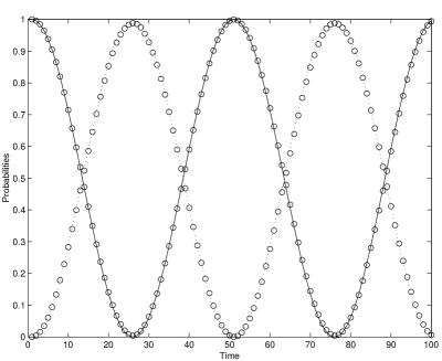
Fig. 1.1: Time-evolution of the probabilities (analytical results) for vacuum $\left|0\right>$ (solid curve) and one-photon state $\left|1\right>$ (dotted curve) for the system with Kerr medium described by the Hamiltonian $\frac{1}{2}\chi(\hat{a}^{\dagger})^{2}\hat{a}^{2}$. The circle marks denote numerical results. The pulse strength is $\epsilon=\pi/50$.

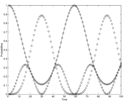
Fig. 1.2: The same as in Fig. 1.1 but for the system with the Kerr medium described by $\frac{1}{3}\chi(\hat{a}^{\dagger})^{3}\hat{a}^{3}$. Analytical results for: vacuum $\left|0\right>$ (solid curve), one-photon state $\left|1\right>$ (dashed curve), and two-photon state $\left|2\right>$ (dotted curve). The numerical results are marked by circles.

assumptions introduced here we deal with the following correspondence:

$$\left.\hat{U}\right|_{\infty}\leftrightarrow\hat{D}$$ (1.47)

To check our analytical formulas derived in the previous sections, we shall concentrate on the two cases where the parameter ${N}=2,3$. First, for ${N}=2$ we apply the evolution operator

$$\hat{U}=\exp\left\{-i\left[\frac{\chi}{2}\left(\hat{a}^{\dagger}\right)^{2}\hat{a}^{2}+\epsilon\left(\hat{a}^{\dagger}+\hat{a}\right)\right]t\right\}$$ (1.48)

and the results are shown in Fig. 1.1, which also shows the analytical results for the probabilities of finding the system in vacuum $\left|0\right>$ and one-photon $\left|1\right>$ states together with those of the numerical method. The analytical and numerical results agree almost perfectly and for these two cases we obtain the well-known oscillatory behavior. Obviously, one should keep in mind that the interaction with the external field is weak ($\epsilon\ll\chi$) and we assume that $\epsilon=\pi/50$ contrary to $\chi=1$.

Analogously, for ${N}=3$ three states are involved in the system evolution. For this case the evolution operator should be of the form

$$\hat{U}=\exp\left(-i\left[\frac{\chi}{3}\left(\hat{a}^{\dagger}\right)^{3}\hat{a}^{3}+\epsilon\left(\hat{a}^{\dagger}+\hat{a}\right)\right]t\right)$$ (1.49)

whereas the parameters $\epsilon$ and $\chi$ are the same as for the case of ${N}=2$. Similarly as for ${N}=2$ the agreement of the analytical results with their numerical counterparts is very good. Thus, Fig. 1.2 depicts oscillations of the probabilities for the states $\left|0\right>$, $\left|1\right>$ and $\left|2\right>$. The amplitude of the oscillations for one-photon state $\left|1\right>$ is considerably smaller than that for other two states involved in the evolution. This fact agrees with the properties of the Fock expansion of the FD coherent state [3].

Applying the numerical method described here, we can also estimate the error of the perturbative treatment introduced in the previous sections. In Fig. 1.3 we show the probability corresponding to the three-photon state $\left|3\right>$ as a function of time. It is seen that the probability oscillates in a similar way as those corresponding to the states $\left|0\right>$, $\left|1\right>$, and $\left|2\right>$. However, the amplitudes of the oscillations differ significantly. Thus, the probability for the state $\left|3\right>$ oscillates between $0$ and $\sim 1.2\times 10^{-3}$ whereas that corresponding to the state $\left|1\right>$ changes its value from $0$ to $\sim 0.3$ (Fig. 1.2). We see that the dynamics of the system described by the Hamiltonian (1.1) is restricted in practice to the closed set of the Fock states. This fact and the behavior of the probabilities shown in Figs. 1.1 and 1.2 proves that the quantum states generated by the system described by Hamiltonian (1.1) are very close to the FD coherent states described in Ref. [3].

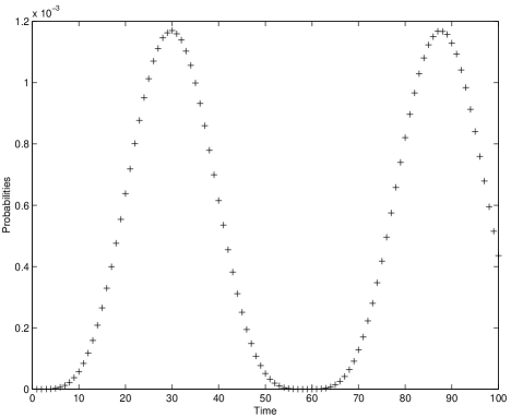
Fig. 1.3: The probability for the three-photon state $\left|3\right>$ obtained from the numerical calculations. All parameters are the same as for Fig. 1.2.

 IV.  State generation in dissipative systems

It is obvious that in the real physical situations we are not able to avoid dissipation processes. For dissipative systems, we cannot take an external excitation too weak (the parameter $\epsilon$ cannot be too small) since the field interacting with the nonlinear oscillator could be completely damped and hence, our model could become completely unrealistic. Moreover, the dissipation in the system leads to a mixture of the quantum states instead of their coherent superpositions.Therefore, we should determine the influence of the damping processes on the systems discussed here. To investigate such processes we can utilize various methods. For instance, the quantum jumps simulations [38] and quantum state diffusion method [39] can be used. Description of these two methods can be found in Ref. [40] where they were discussed and compared. Another way to investigate the damping processes is to apply the approach based on the density matrix formalism. Here, we shall concentrate on this method [41, 42, 12].

As we have discussed earlier, the time dependence of the envelope of external excitation does not influence the final analytical result discussed here. The parameter $f(t)$ appears only inside the integral determining the external pulse area $\theta(t)$ [Eq. 1.10]. Therefore, we can assume without losing generality of our considerations that the excitation is in the form of a series of ultrashort pulses. Then the function $f(t)$ can be modeled by the Dirac-delta functions as

$$f(t) = \sum_{k=0}^{\infty}\delta(t-kT)$$ (1.50)

where $T$ is a time between two subsequent pulses. For such situation the time-evolution of the system can be divided into two different stages. When the damping processes are absent, the first stage is a “free” evolution of the nonlinear oscillator determined by the unitary evolution operator

$$\hat{U}_{\mathrm{N}L} = \exp\left[-i\frac{\chi T}{2}\left(\hat{a}^{\dagger}\right)^{2}\hat{a}^{2}\right]$$ (1.51)

We assume the simplest case, where the time-evolution is restricted to two quantum states $\left|0\right>$ and $\left|1\right>$. The second stage of the time-evolution of the system is caused by its interaction with an infinitely short external pulse. This part of the evolution is described by the second term of the Hamiltonian (1.1) and can be described by the following evolution operator

$$\hat{U}_{\mathrm{K}} = \exp\left[-i\epsilon\left(\hat{a}^{\dagger}+\hat{a}\right)\right]$$ (1.52)

The overall evolution of the system can be described as a subsequent action of the operators $\hat{U}_{\mathrm{N}L}$ and $\hat{U}_{\mathrm{K}}$ on the initial state. When we take into account losses during the time-evolution between two pulses we should solve the appropriate master equation. It can be written as

$$\frac{d\rho}{dt}=-i\frac{\chi}{2}\left(\hat{a}^{\dagger}\right)^{2}\hat{a}^{2}+\frac{\gamma}{2}\left(2\hat{a}\rho\hat{a}^{\dagger}-\hat{a}^{\dagger}\hat{a}\rho-\rho\hat{a}^{\dagger}\hat{a}\right)$$ (1.53)

The solution of this master equation in the Fock number states basis is given by [41, 42]

$$\left<p\right|\rho(t+T)\left|q\right>=\exp\left[i\frac{\vartheta}{2}(p-q)\right]\frac{[g(T)]^{(p+q)/2}}{\sqrt{p!q!}}\sum_{n=p}^{\infty}\left<n\right|\rho(t)\left|n-(p-q)\right>$$

$$\times\frac{\sqrt{n![n-(p-q)]!}}{(n-p)!}(1+i\delta)^{-(n-p)}\left[1-g(T)\right]^{(n-p)}\quad\quad$$ (1.54)

where

$$\delta = \frac{p-q}{\kappa}$$

$$g(T) = \exp\left[-\kappa\vartheta-i\vartheta(p-q)\right]$$

$$\kappa = \frac{\gamma}{\chi}$$

$$\vartheta = \chi T$$ (1.55)

The symbol $\gamma$ appearing above is a damping constant responsible for the cavity loss. Thus solving the master equation (1.53) we can determine the probabilities of finding the system in an arbitrary $n$-photon state. Of course, the evolution during single ultrashort, external pulse is determined by the operator $\hat{U}_{K}$ as before.

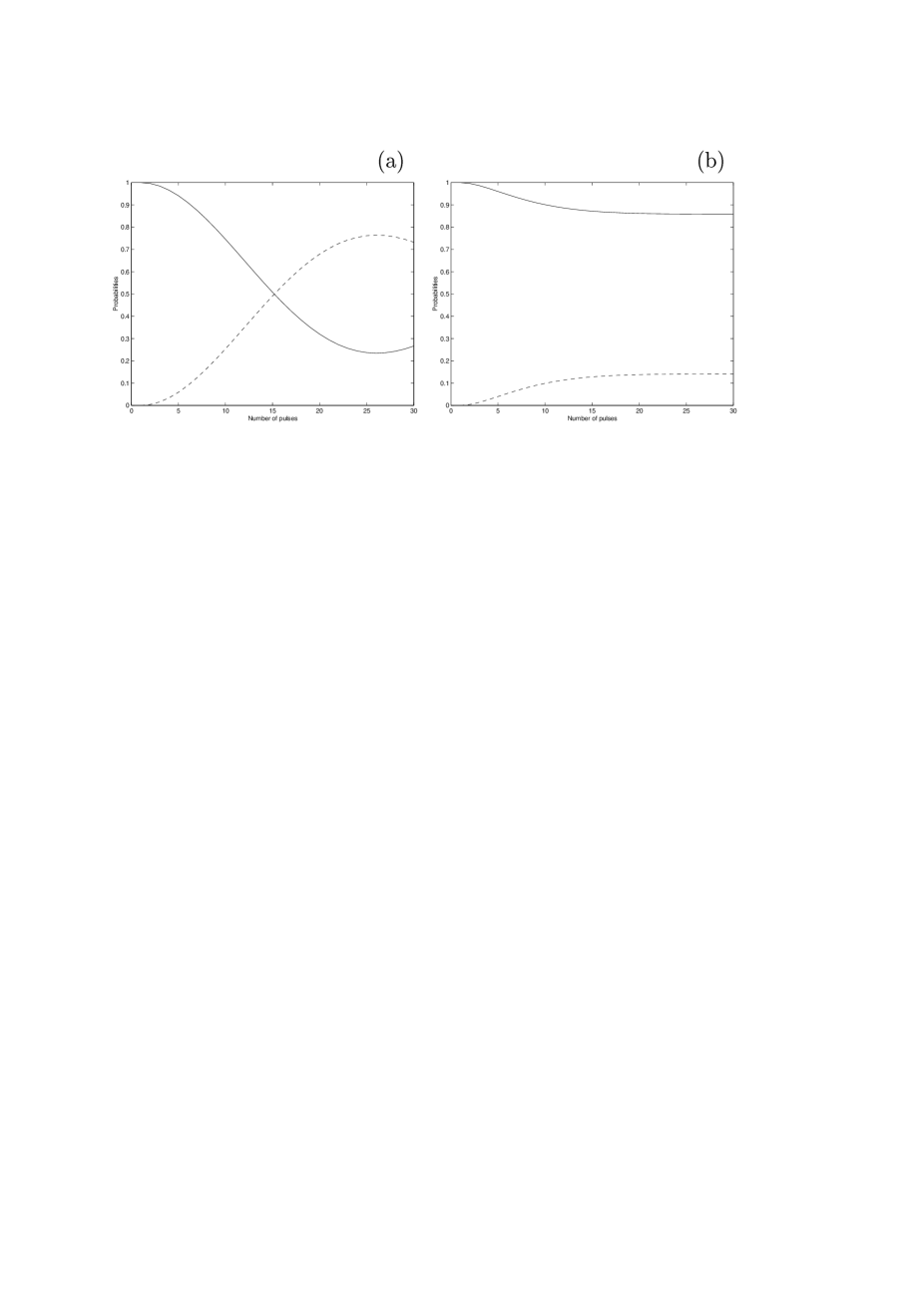
Fig. 1.4: The probabilities for vacuum $\left|0\right>$ (solid curve) and one-photon state $\left|1\right>$ (dashed curve) for the Kerr medium described by $\frac{1}{2}\chi(\hat{a}^{\dagger})^{2}\hat{a}^{2}$. The damping constants are: (a) $\gamma=0.01$ and (b) $\gamma=0.1$. The pulse strength is $\epsilon=\pi/50$ and the time $T=\pi$.

Thus Fig. 1.4 shows probabilities for vacuum $\left|0\right>$ and one-photon $\left|1\right>$ state for weak external excitation once more. We have chosen two values of the damping parameter: $\gamma=0.1$ (Fig. 1.4(a)) and $\gamma=0.01$ (Fig. 1.4(b)). It is seen that for weak damping we observe slow oscillations of the probabilities, similarly as for the case of the quantum nonlinear oscillator without dissipation. Moreover, for ($\gamma=0.01$) the amplitude of the oscillations reaches over $75\%$ of its value for the case of $\gamma=0$. As a consequence, we are able to get the field very close to the desired quantum state. However, as the damping increases the situation changes considerably. For $\gamma=0.1$ the oscillations of the probabilities vanish, and the resulting state is far from the FD coherent state defined in the two-dimensional Hilbert space. We see that the dissipation in the system can drastically lower the effectiveness of producing the FD coherent states. Nevertheless, one should keep in mind one of the crucial points of our considerations: the assumption of weak external excitation. Hence, we hope that for sufficiently weak damping, our system can evolve to a state that is very close the quantum state of our interest.

  V.  Generalized method for FD squeezed vacuum generation

The method described in the previous sections can be easily generalized to be useful for generation of various FD quantum-optical states different from the FD coherent state. Thus, we shall show an example of how to adapt our method to generate the FD squeezed vacuum [10]. In the first part of this work [see Eq. (78) in Ref. [1]], we have defined the $(s+1)$-dimensional generalized squeezed vacuum to be

$$\left|\xi\right>_{(s)}=\exp\left[\frac{\xi}{2}(\hat{a}_{s}^{\dagger})^{2}-\frac{\xi^{*}}{2}\hat{a}_{s}^{2}\right]|0\rangle$$ (1.56)

where $\xi=|\xi|\exp(i\phi)$ is the complex squeeze parameter, whereas $\hat{a}_{s}$ and $\hat{a}_{s}^{\dagger}$ are, respectively, the FD annihilation and creation operators defined by (1.21). Since the properties of the FD squeezed vacuum have already been discussed [1], here we shall concentrate on the method of its generation.

We assume that our system consists of a Kerr medium of the $(s+1)$th-order nonlinearity and a parametric amplifier driven by a series of ultrashort external classical-light pulses. Thus, the Hamiltonian describing our system can be written in the interaction picture as

$$\hat{H}=\frac{\chi}{(s+1)}\left(\hat{a}^{\dagger}\right)^{s+1}\hat{a}^{s+1}+\epsilon\left(\hat{a}^{\dagger 2}+\hat{a}^{2}\right)f(t)$$ (1.57)

where the first term describes the $(s+1)$-photon nonlinear oscillator (Kerr medium) as in (1.11), and the second term represents a pulsed parametric oscillator modulated by $f(t)$, given by (1.50). This situation differs from those discussed in the previous sections in one important point, namely, in the character of external excitation. For this case we assume that the oscillator is driven by a second-order parametric process instead of linear excitation involved in the FD coherent-state generation. The model, described by (1.57) with the two-photon Kerr Hamiltonian, was studied by Milburn and Holmes [42] in their analysis of quantum coherence and classical chaos. The system for $s=1$ and $f(t)=1$ is referred to as the Cassinian oscillator and has been analyzed in the context of squeezing by, for instance, Gerry et al. [43] and DiFilippo et al. [44]. The time evolution of the system leads to the generation of the quantum states that differ significantly from the FD coherent states. In a similar way as for the generation of the latter, we assume that the excitation is weak ($\epsilon\ll\chi$), and we can apply the perturbative treatment again. As a consequence, we get the formula for the $n$-photon state expansion

$$\left|\phi(t)\right>=\sum_{n=0}^{\sigma}C_{2n}(t)\left|2n\right>+\epsilon C_{2\sigma+2}(t)\left|2\sigma+2\right>+O(\epsilon^{2})$$ (1.58)

where the expansion coefficients $C_{2n}=\left<2n\right|\left.\phi(t)\right>$ for $n=0,\dots,\sigma$ are

$$C_{2n}(t)=(-1)^{n}\frac{(2\sigma)!}{\sqrt{(2n)!}}\sum_{k=0}^{\sigma}\exp(ix_{k}\epsilon t)\frac{G_{n}(x_{k})}{G_{\sigma}(x_{k})G^{\prime}_{\sigma+1}(x_{k})}$$ (1.59)

and

$$C_{2\sigma+2}(t)=2^{-\sigma-1}\sqrt{(2\sigma+1)(2\sigma+2)}\,C_{2\sigma}(t)$$ (1.60)

The functions $G_{n}(x)$ appearing above are the Meixner–Sheffer orthogonal polynomials; the prime sign in Eq. (1.59) denotes their $x$-derivative, and $\sigma={\mathrm{I}nt}(s/2)$ is the integer part of $s/2$. If we omit the terms proportional to $\epsilon$ and higher, we get the expansion for the FD squeezed vacuum as

$$\left|\xi=-2\epsilon t\right>_{(s)}=\left|\phi(t)\right>+O(\epsilon)$$ (1.61)

So, our system evolves to a state close to the FD squeezed vacuum discussed in Ref. [10].

VI.  Summary

We have discussed one of the possible methods of generation of the FD quantum-optical states. Although, it is possible to generate $n$-photon Fock states and then to construct a desired state from these states, we have concentrated on the generation schemes that can lead directly to the FD coherent states and FD squeezed vacuum. The method described here is based on the quantum nonlinear oscillator evolution. We have assumed that this oscillator is driven by an external excitation. We have shown that within the weak excitation regime we are able to generate with high accuracy the appropriate FD quantum state. Thus, depending on the character of the excitation we can produce various FD states. For instance, for the linear excitation case we generate the FD coherent state, whereas for the parametric excitation of the FD squeezed vacuum can be achieved. Moreover, we have shown that the mechanism of the generation does not depend on the shape of the excitation envelope. Hence, various forms of the latter can be assumed depending of the feasibility of our model from the experimental or mathematical point of view.

For the situations discussed here appropriate analytical formulas for the generated states have been derived. These results have been obtained within the perturbation theory, and they agree with those of the $n$-photon expansion of the appropriate FD states. Moreover, we have proposed methods for checking our results numerically, and we have shown that numerical results agree very well with the analytical ones. Since, we are not able to avoid dissipation processes from real physical situations, we have discussed damping processes two. It has been shown that although dissipation can play crucial role in the whole system dynamics and is able to destroy the effect of the FD state generation completely, under special assumptions these states can be achieved.

ACKNOWLEDGMENTS

The authors thank J. Bajer, S. Dyrting, N. Imoto, M. Koashi, T. Opatrný, Ş. K. Özdemir, J. Peřina, K. Pia̧tek and R. Tanaś for their helpful discussions. A. M. is indebted to Prof. Nobuyuki Imoto for his hospitality and stimulating research at SOKEN.

REFERENCES

Index

Cassinian oscillator, 14

Coherent states; generalized, 7

Coherent states; two-dimensional, 2

Displacement operator, 8

Dissipative systems, 10

Finite-dimensional Hilbert space, 1

Hermite polynomial, 6

Kerr medium, 2

Meixner–Sheffer orthogonal polynomials, 14

Rotating wave approximation, 4

Squeezed vacuum; generalized, 13

REFERENCES

- 1. A. Miranowicz, W. Leoński, and N. Imoto, “Quantum-optical states in finite-dimensional Hilbert space. I. General formalism”, Chapter 3, this volume.
- 2. V. Bužek, A. D. Wilson-Gordon, P. L. Knight, and W. K. Lai, Phys. Rev. A 45, 8079 (1992).
- 3. A. Miranowicz, K. Pia̧tek, and R. Tanaś, Phys. Rev. A 50, 3423 (1994); T. Opatrný, A. Miranowicz, and J. Bajer, J. Mod. Opt. 43, 417 (1996).
- 4. L. M. Kuang, F. B. Wang, and Y. G. Zhou, Phys. Lett. 183, 1 (1993) and J. Mod. Opt. 42, 1307 (1994); A. K. Pati and S. V. Lawande, Phys. Rev. A 51, 5012 (1995); B. Roy and R. Roychoudhury, Int. J. Theor. Phys. 36, 1525 (1997); B. Roy, Modern Phys. Lett. 11, 963 (1997).
- 5. A. Miranowicz, T. Opatrný, and J. Bajer, in T. Hakioǧlu and A. S. Shumovsky (Eds.), Quantum Optics and the Spectroscopy of Solids: Concepts and Advances, Ser. on Fundamental Theories in Physics, Kluwer, Dordrecht, 1997, p. 225.
- 6. B. Roy and P. Roy, J. Phys. A 31, 1307 (1998).
- 7. J. Y. Zhu and L. M. Kuang, Phys. Lett. A 193, 227 (1994).
- 8. D. Pegg and S. M. Barnett, Phys. Rev. A 41, 3427 (1989); S. M. Barnett and D. T. Pegg, J. Mod. Opt. 36, 7 (1989).
- 9. K. Wódkiewicz, P. L. Knight, S. J. Buckle, and S. M. Barnett, Phys. Rev. A 35, 2567 (1987); P. Figurny, A. Orłowski, and K. Wódkiewicz, Phys. Rev. A 47, 5151 (1993); D. J. Wineland, J. J. Bollinger, W. M. Itano, and D. J. Heinzen, Phys. Rev. A 50, 67 (1994).
- 10. A. Miranowicz, W. Leoński, and R. Tanaś, in D. Han et al. (Eds.), NASA Conference Publication 206855, Greenbelt, MD, 1998, p. 91.
- 11. J. R Kukliński, Phys. Rev. Lett. 64, 2507 (1990).
- 12. W. Leoński and R. Tanaś, Phys. Rev. A 49, R20 (1994).
- 13. W. Leoński, S. Dyrting, and R. Tanaś, J. Mod. Opt. 44, 2105 (1997).
- 14. J. Krause, M. O. Scully, T. Walther, and H. Walther, Phys. Rev. A 39, 1915 (1989); M. Kozierowski and S. M. Chumakov, Phys. Rev. A 52, 4194 (1995); P. Domokos, M. Brune, J. M Raimond, and S. Haroche, Eur. Phys. J. 1, 1 (1998).
- 15. G. M. D’Ariano, L. Maccone, M. G. A. Paris, and M. F. Sacchi, Phys. Rev. A 61, 053817 (2000).
- 16. S. Bose, K. Jacobs, and P. L. Knight, Phys. Rev. A 56, 4175 (1997).
- 17. D. T. Pegg, L. S. Philips, and S. M. Barnett, Phys. Rev. Lett. 81, 1604 (1998).
- 18. M. Koniorczyk, Z. Kurucz, A. Gábris, and J. Janszky, Phys. Rev. A 62, 013802 (2000); M. G. A. Paris, ibid. 033813;A. Miranowicz, Ş. K. Özdemir, N. Imoto, and M. Koashi, Mtg. Abstr. Phys. Soc. Jpn. 62, 108 (2000).
- 19. M. Brune, S. Haroshe, V. Lefevre, J. M. Raimond, and N. Zagury, Phys. Rev. Lett. 65, 976 (1990); M. J. Holland, D. F. Walls, and P. Zoller, Phys. Rev. Lett. 67, 1716 (1991).
- 20. K. Vogel, V. M. Akulin, and W. P. Schleich, Phys. Rev. Lett. 71, 1816 (1993); B. M. Garraway, B. Sherman, H. Moya-Cessa, P. L. Knight, and G. Kurizki, Phys. Rev. A 49, 535 (1994); J. Janszky, P. Domokos, S. Szabó, and P. Adam, Phys. Rev. A 51, 4191 (1995); M. Dakna, J. Clausen, L. Knöll, D.-G. Welsch, Phys. Rev. A 59, 1658 (1999).
- 21. Special issue on quantum state preparation and measurement, J. Mod. Opt. 44 (11/12) (1997).
- 22. W. Leoński, Phys. Rev. A 54, 3369 (1996).
- 23. A. Miranowicz, K. Pia̧tek, and T. Opatrný and R. Tanaś, Acta. Phys. Slov. 45, 391 (1995).
- 24. W. Leoński, Phys. Rev. A 55, 3874 (1997).
- 25. Y. Yamamoto, N. Imoto, and S. Machida, Phys. Rev. A 33, 3243 (1986).
- 26. M. Kitagawa and Y. Yamamoto, Phys. Rev. A 34, 3974 (1986).
- 27. A. D. Wilson-Gordon, V. Bužek, and P. L. Knight, Phys. Rev. A 44, 7647 (1991).
- 28. B. Yurke and D. Stoller, Phys. Rev. Lett. 57, 13 (1986).
- 29. P. Tombessi and A. Mecozzi, J. Opt. Soc. Am. B 4, 1700 (1987).
- 30. A. Miranowicz, R. Tanaś, and S. Kielich, Quantum Opt. 2, 253 (1990).
- 31. V. Bužek, G. Drobný, M. S. Kim, G. Adam, and P. L. Knight, Phys. Rev. A 56, 2352 (1997).
- 32. S. Walentowitz and W. Vogel, Phys. Rev. A 55, 4438 (1997); ibid. 58, 679 (1998); S. Walentowitz, W. Vogel, and P. L. Knight, Phys. Rev. A 59, 531 (1999).
- 33. A. Miranowicz, W. Leoński, S. Dyrting, and R. Tanaś, Acta Phys. Slov. 46, 451 (1996).
- 34. L. Allen and J. H. Eberly, Optical Resonance and Two-Level Atoms, Wiley, New York, 1975.
- 35. C. C. Gerry, Phys. Lett. A 124, 237 (1987); V. Bužek and I. Jex, Acta Phys. Slov. 39, 351 (1989); M. Paprzycka and R. Tanaś, Quantum Opt. 4, 331 (1992).
- 36. W. H. Press, B. P. Flannery, S. A. Teukolsky, and W. T. Vetterling, Numerical Recipes. The Art of Scientific Computing, Cambridge Univ. Press, 1986.
- 37. R. J. Glauber, Phys. Rev. A 131, 2766 (1963).
- 38. J. Dalibard, Y. Castin, and K. Mölmer, Phys. Rev. Lett. 68, 580 (1992); K. Mölmer, Y. Castin, and J. Dalibard, J. Opt. Soc. Am. 10, 524 (1993); H. J. Carmichael, An Open Systems Approach to Quantum Optics, Lecture Notes in Physics, Series, Springer, Berlin, 1993.
- 39. N. Gisin and I. C. Percival, J. Phys. A 25, 5677 (1992); ibid 26, 2233 and 2245 (1993).
- 40. B. M. Garraway and P. L. Knight, Phys. Rev. A 49, 1266 (1994).
- 41. G. J. Milburn and C. A. Holmes, Phys. Rev. Lett. 56, 2237 (1986).
- 42. G. J. Milburn and C. A. Holmes, Phys. Rev. A 44, 4704 (1991).
- 43. C. C. Gerry and S. Rodrigues, Phys. Rev. A 36, 5444 (1987); C. C. Gerry, R. Grobe, and E. R. Vrscay, Phys. Rev. A 43, 361 (1991).
- 44. F. DiFilippo, V. Natarajan, K. R. Boyce, and D. E. Pritchard, Phys. Rev. Lett. 68, 2859 (1992).
Index