A Note on Linear Optics Gates by Post-Selection

Abstract

Recently it was realized knill:qc2000e that linear optics and photo-detectors with feedback can be used for theoretically efficient quantum information processing. The first of three steps toward efficient linear optics quantum computation (eLOQC) was to design a simple non-deterministic gate, which upon post-selection based on a measurement result implements a non-linear phase shift on one mode. Here a computational strategy is given for finding non-deterministic gates for bosonic qubits with helper photons. A more efficient conditional sign flip gate is obtained.

I Introduction

Now that we know that linear optics and photo-detectors are sufficient for quantum information processing knill:qc2000e , it is necessary to investigate how the necessary schemes can be realized more efficiently. One promising direction is to use superpositions of squeezed or coherent states for encoding qubits gottesman:qc2000a ; ralph:qc2002b . In this note, it is shown how the non-deterministic gates at the foundation of the constructions in knill:qc2000e can be found and improved. Other relevant work in this direction includes ralph:qc2001a ; rudolph:qc2001a ; pittman:qc2001a ; pittman:qc2001b , where networks suitable for experimental realization are given. The focus of this paper is on what can be done in principle without giving experimentally accessible layouts. To that end, a systematic method is given for finding non-deterministic gates based on a combination of algebraic solution finding, exploitation of known symmetries, and numerical optimization. By using the method, a conditional sign flip for bosonic qubits that succeeds with probability $1/13.5$ using two helper photons is found. This improves the one in knill:qc2000e , which succeeds with probability $1/16$. What is the optimum probability of success for any number of helper photons? A characterization of the achievable states without post-selection implies that the probability cannot be one, a result related to known bounds on Bell-measurements lutkenhaus:qc1999a ; calsamiglia:qc2001a .

II Preliminaries

The physical system of interest consists of bosonic modes, each of whose state space is spanned by the number states $\mbox{$|||$}{0}\mbox{$\rangle\rangle\rangle$},\mbox{$|||$}{1}\mbox{$\rangle\rangle\rangle$},\mbox{$|||$}{2}\mbox{$\rangle\rangle\rangle$},\ldots$. If more than one mode is used, they are distinguished by labels. For example, $\mbox{$|||$}{k}\mbox{$\rangle\rangle\rangle$}_{{}_{\!\!{\scriptstyle\mathsf{r}}}}$ is the state with $k$ photons in the mode labeled $\mathsf{r}$. The hermitian transpose of this state is denoted by ${}^{\scriptstyle\mathsf{r}}\!\mbox{$\langle\langle\langle$}{k}\mbox{$|||$}$. The vacuum state for a set of modes has each mode in the state $\mbox{$|||$}{0}\mbox{$\rangle\rangle\rangle$}$ and is denoted by $\mbox{$|||$}{{\mathbf{0}}}\mbox{$\rangle\rangle\rangle$}$. The anniliation operator for mode $r$ is written as ${{\mathbf{a}}}^{({\mathsf{r}})}$ and the creation operator as ${{\mathbf{c}}}^{({\mathsf{r}})}=\left({{\mathbf{a}}}^{({\mathsf{r}})}\right)^{\dagger}$. Recall that ${{\mathbf{c}}}^{({\mathsf{r}})}\mbox{$|||$}{m}\mbox{$\rangle\rangle\rangle$}=\sqrt{m+1}\mbox{$|||$}{m+1}\mbox{$\rangle\rangle\rangle$}$. Labels are omitted when no ambiguity results. Hamiltonians that are at most quadratic in creation and annihilation operators generate the group of linear optics transformations. Among these, the ones that preserve the particle number are called passive linear. Every passive linear optics transformation can be achieved by a combination of beam splitters and phase shifters. If $U$ is passive linear, then $U{{\mathbf{c}}}^{({\mathsf{r}})}\mbox{$|||$}{{\mathbf{0}}}\mbox{$\rangle\rangle\rangle$}=\sum_{s}u_{sr}{{\mathbf{c}}}^{({\mathsf{s}})}\mbox{$|||$}{{\mathbf{0}}}\mbox{$\rangle\rangle\rangle$}$, where $u_{sr}$ defines a unitary matrix $\hat{u}$. Conversely, for every unitary matrix $\hat{u}$, there is a corresponding passive linear optics transformation reck:qc1994a . For the remainder of this note, all linear optics transformations are assumed to be passive.

III Conditional phase shifts

A conditional phase shift by $\theta$ on two modes is the map $\mathsf{CS}_{\theta}:\mbox{$|||$}{ab}\mbox{$\rangle\rangle\rangle$}\rightarrow e^{i(ab)\theta}\mbox{$|||$}{ab}\mbox{$\rangle\rangle\rangle$}$ for $0\leq a,b\leq 1$. These phase shifts can be used to implement conditional phases on two bosonic qubits. A bosonic qubit $\mathsf{Q}_{\mathsf{r},\mathsf{s}}$ is defined by identifying logical $\mbox{$|||$}{\mathfrak{0}}\mbox{$\rangle\rangle\rangle$}$ with $\mbox{$|||$}{01}\mbox{$\rangle\rangle\rangle$}_{{}_{\!\!{\scriptstyle\mathsf{rs}}}}$ and logical $\mbox{$|||$}{\mathfrak{1}}\mbox{$\rangle\rangle\rangle$}$ with $\mbox{$|||$}{10}\mbox{$\rangle\rangle\rangle$}_{{}_{\!\!{\scriptstyle\mathsf{rs}}}}$. The modes $\mathsf{r}$ and $\mathsf{s}$ can be two distinct spatial modes or the two polarizations of one spatial mode. To realize the conditional sign flip between $\mathsf{Q}_{\mathsf{1},\mathsf{2}}$ and $\mathsf{Q}_{\mathsf{3},\mathsf{4}}$, apply $\mathsf{CS}_{180^{\circ}}$ to modes $\mathsf{1}$ and $\mathsf{3}$. The bosonic qubit controlled-not can then be implemented using conditional sign flips and single qubit rotations, which are realizable with beamsplitters.

In knill:qc2000e , conditional sign flips were implemented indirectly using a non-deterministic realization of the map

$$\mathsf{NS}:\alpha\mbox{$|||$}{0}\mbox{$\rangle\rangle\rangle$}+\beta\mbox{$|||$}{1}\mbox{$\rangle\rangle\rangle$}+\gamma\mbox{$|||$}{2}\mbox{$\rangle\rangle\rangle$}\rightarrow\alpha\mbox{$|||$}{0}\mbox{$\rangle\rangle\rangle$}+\beta\mbox{$|||$}{1}\mbox{$\rangle\rangle\rangle$}-\gamma\mbox{$|||$}{2}\mbox{$\rangle\rangle\rangle$}$$ (1)

that succeeds with probability $1/4$. This realization requires one helper photon and two ancilla modes. The goal is to implement $\mathsf{CS}_{\theta}$ more efficiently directly using two helper photons. One helper photon can be shown to be insufficient by means of the same algebraic method about to be used. Let modes $\mathsf{1}$ and $\mathsf{2}$ contain the state to which $\mathsf{CS}_{\theta}$ is to be applied. The basic scheme is to start with two ancilla modes $\mathsf{3}$ and $\mathsf{4}$ initialized with one photon each, apply a linear optics transformation to modes $\mathsf{1},\mathsf{2},\ldots,\mathsf{k}$ with $k\geq 4$, measure all but the first two of these modes and accept only a predetermined outcome, say where one photon is detected in each of modes $\mathsf{3}$ and $\mathsf{4}$ and none in the added modes. Let $\hat{u}$ be the unitary matrix associated with the linear optics transformation, with $u_{sr}$ the entries of $\hat{u}$. The post-selected final state is determined completely by the $4\times 4$ upper left submatrix $V$ of $\hat{u}$ with entries $V_{rs}=u_{sr}$ for $s,r\leq 4$.

It is necessary to consider the effects of the scheme on the initial states $\mbox{$|||$}{00}\mbox{$\rangle\rangle\rangle$}_{{}_{\!\!{\scriptstyle\mathsf{12}}}},\mbox{$|||$}{01}\mbox{$\rangle\rangle\rangle$}_{{}_{\!\!{\scriptstyle\mathsf{12}}}},\mbox{$|||$}{10}\mbox{$\rangle\rangle\rangle$}_{{}_{\!\!{\scriptstyle\mathsf{12}}}},\mbox{$|||$}{11}\mbox{$\rangle\rangle\rangle$}_{{}_{\!\!{\scriptstyle\mathsf{12}}}}$. Since photon number is conserved, we have, without renormalization:

$$\mbox{$|||$}{00}\mbox{$\rangle\rangle\rangle$}_{{}_{\!\!{\scriptstyle\mathsf{12}}}} \rightarrow \alpha_{0000}\mbox{$|||$}{00}\mbox{$\rangle\rangle\rangle$}_{{}_{\!\!{\scriptstyle\mathsf{12}}}}$$ (2)

$$\mbox{$|||$}{01}\mbox{$\rangle\rangle\rangle$}_{{}_{\!\!{\scriptstyle\mathsf{12}}}} \rightarrow \alpha_{0101}\mbox{$|||$}{01}\mbox{$\rangle\rangle\rangle$}_{{}_{\!\!{\scriptstyle\mathsf{12}}}}+\alpha_{0110}\mbox{$|||$}{10}\mbox{$\rangle\rangle\rangle$}_{{}_{\!\!{\scriptstyle\mathsf{12}}}}$$ (3)

$$\mbox{$|||$}{10}\mbox{$\rangle\rangle\rangle$}_{{}_{\!\!{\scriptstyle\mathsf{12}}}} \rightarrow \alpha_{1010}\mbox{$|||$}{10}\mbox{$\rangle\rangle\rangle$}_{{}_{\!\!{\scriptstyle\mathsf{12}}}}+\alpha_{1001}\mbox{$|||$}{01}\mbox{$\rangle\rangle\rangle$}_{{}_{\!\!{\scriptstyle\mathsf{12}}}}$$ (4)

$$\mbox{$|||$}{11}\mbox{$\rangle\rangle\rangle$}_{{}_{\!\!{\scriptstyle\mathsf{12}}}} \rightarrow \alpha_{1111}\mbox{$|||$}{11}\mbox{$\rangle\rangle\rangle$}_{{}_{\!\!{\scriptstyle\mathsf{12}}}}+\alpha_{1120}\mbox{$|||$}{20}\mbox{$\rangle\rangle\rangle$}_{{}_{\!\!{\scriptstyle\mathsf{12}}}}+\alpha_{1102}\mbox{$|||$}{02}\mbox{$\rangle\rangle\rangle$}_{{}_{\!\!{\scriptstyle\mathsf{12}}}}$$ (5)

To be successful, the amplitudes have to satisfy

$$\alpha_{0110}=\alpha_{1001}=\alpha_{1120}=\alpha_{1102}=0$$ (6)

$$\alpha_{1010}=\alpha_{0101}=\alpha_{0000}$$ (7)

$$\alpha_{1111}=e^{i\theta}\alpha_{0000}$$ (8)

The amplitudes are polynomials of the coefficients of $V$. For example $\alpha_{0000}=v_{33}v_{44}+v_{34}v_{43}$. More generally, define $p_{s}=\sum_{r}v_{rs}{{\mathbf{c}}}^{({\mathsf{r}})}$. If the initial state in mode $\mathsf{s}$ has $d_{s}$ photons, then the output state is given by $P=\prod_{s}p_{s}^{d_{s}}$. Thus, $P$ is a polynomial of the ${{\mathbf{c}}}^{({\mathsf{r}})}$. If $\beta$ is the coefficient of the monomial $\prod_{t}\left({{\mathbf{c}}}^{({\mathsf{t}})}\right)^{m_{t}}$ in $P$, then the output amplitude for having $m_{t}$ photons in mode $\mathsf{t}$ is given by $\sqrt{\prod_{t}m_{t}!}\beta$. This shows that the amplitudes $\alpha_{abcd}$ are polynomials of the $v_{rs}$.

The first step for constructing $\mathsf{CS}_{\theta}$ is to solve Eqs. 6–8, which are polynomial identites in the $v_{rs}$. Before showing how to reduce the difficulty of doing that, let us see how to proceed from there. Since there are $16$ free complex variables, the solution will have a number of remaining free variables that must be chosen to optimize the probability of success ($|\alpha_{0000}|^{2})$ and to satisfy one more constraint: The solution is an (explicit) matrix $V$ that needs to be extended to a unitary matrix $\hat{u}$. This is possible if and only if the maximum singular value (that is the square root of the maximum eigenvalue of $V^{\dagger}V$) is at most one. The extension is not unique. One can set the first four columns of $\hat{u}$ to the matrix with orthonormal columns

$$X=\left(\begin{array}[]{cc}V&\\ (\textbf{I}-V^{\dagger}V)^{1/2}&\end{array}\right),$$ (9)

and then complete the last four columns with any orthonormal basis of the orthogonal complement of the space spanned by the columns of $X$. The maximum singular value constraint is needed to be able to compute the square root in the expression for $X$. If some of the singular values of $V$ are equal to one, then fewer than four additional columns and rows can be used

The singular value constraint cannot be easily achieved using algebraic methods. In principle, one can reparametrize the matrix $V$ to guarantee the constraint, for example by using the polar decomposition and an Euler angle representation of unitary matrices. In the case where $\mathsf{CS}_{\theta}$ is to be applied to the “left” modes of a pair of bosonic qubits, the singular value constraint can be removed by exploiting a rescaling symmetry. Now there are two additional modes to complete the bosonic qubits. The total number of photons is always four. Let $V$ be a matrix whose coefficients satisfy the identities for the $\alpha_{abcd}$. Let $\lambda=\lambda(V)$ be the maximum singular value of $V$ and consider the matrix

$$V_{e}={1\over\lambda}\left(\begin{array}[]{cc}\textbf{I}&\mathbf{0}\\ \mathbf{0}&V\end{array}\right),$$ (10)

where the first two indeces are associated with the two other (“right”) qubit modes. $V_{e}$ has maximum singular value $1$ and can be extended to a unitary $\hat{u}_{e}$ as before. The claim is that if the resulting optics operation is applied to the pair of bosonic qubits with the same post-selection procedure, it has the intended effect with probability $1/\lambda^{8}$. To see that this is true, first observe that, $V^{\prime}=\lambda V_{e}$ satisfies the polynomial equations obtained by requiring that the operation works correctly for the pair of bosonic qubits. The amplitudes (as in Eqs. 2–5) that occur in these equations are polynomials which are either homogenous linear in the coefficients of a given column of $V^{\prime}$ or independent of them. This is because the input states have at most one photon in each mode. Because each input state under consideration has exactly four photons, the amplitudes are all homogenous of degree four in the coefficients of $V^{\prime}$. This implies that multiplying $V^{\prime}$ by $\delta$ scales the amplitudes by $\delta^{4}$. Since the equations to be satisfied are homogenous linear in the amplitudes, every scalar multiple of the matrix also satisfies the equations.

With the observation of the previous paragraph, instead of trying to satisfy the singular value constraint, one can recalculate the probability of success by dividing $V$’s probability of success by $\lambda^{8}$ and optimize it. Note that this works even if $\lambda<1$. In computer experiments using naive optimization methods (see below), this usually led to solutions $V$ with $\lambda=1$ for $\theta=180^{\circ}$ and $\theta=90^{\circ}$.

To simplify solving the equations for the $\alpha_{abcd}$, one can use scaling symmetries to standardize $V$. Since each of the $\alpha_{abcd}$ is homogenous in the variables associated with any one row or column of $V$, the equations of the form $\alpha_{abcd}=0$ are satisfied for any rescaling of a row or column. The non-zero $\alpha_{abcd}$ are homogenous of degree one in the third and fourth column (because of the presence of the helper photons at the input in modes $\mathsf{3}$ and $\mathsf{4}$) and in the third and fourth row (because of the post-conditioning on detecting exactly one photon in each of modes $\mathsf{3}$ and $\mathsf{4}$). Because Eqs. 7–8 are homogenous linear in the amplitudes, rescaling these rows or columns preserves the identities. The non-zero $\alpha_{abcd}$ satisfy that they are of equal degree and homogenous in the first column and (separately) in the first row. This is due to the fact that when a photon is present in mode $\mathsf{1}$ at the input, this is designed to be the case at the output too. Thus multiplying the first column by $\delta$ and the first row by $1/\delta$ does not change the values. Similarly, this rescaling can be used on the second column and row.

The scaling rules of the previous paragraph can be used to introduce unconstrained scaling variables and standardize the entries of $V$. For example, one can take $v_{13}=v_{24}=v_{33}=v_{44}=v_{43}=1$. Note that this choice implies that solutions where any one of these variables is $0$ are not easily found. It may therefore be necessary to try solving with some of the variables set to $0$. For example, the $\mathsf{CS}$ gate of knill:qc2000e after translation into the form used here satisfies $v_{43}=0$. I did not find any solutions satisfying this constraint with better probability of success.

Mathematica was used to solve the equations (any other computer algebra system would do equally well). The strategy was to solve linear equations first and then to simplify expressions. Some Mathematica notes are included verbatim in App. A and include formulas for the solution found. The solution could be expressed in terms of the remaining variables of the last two columns of $V$ and one additional variable. After some experimentation, it seemed that in all the best solutions, $v_{11}=v_{22}$. This was exploited in the final version of the optimization procedure, implemented in Matlab (the programs are available by request). Briefly, the function to be optimized takes as input the remaining free complex variables ($v_{14},v_{23},v_{34},l_{1}$), and a non-redundant subset of the scaling variables. To avoid infinities, one can provide the logarithms of the scaling variables as inputs. The scales can be taken to be real since phases have no effect on the probability of success. The function can then be optimized using random starting points. With the optimization procedures provided by Matlab, it was found useful to randomly perturb the point returned and repeat until the solution no longer changes significantly. This procedure routinely finds the same optimum. For $\theta=180^{\circ}$, it was possible to guess the algebraic numbers that it converged to. Here is a version of the matrix found, which turns out to be unitary:

$$V_{180^{\circ}}=\left(\begin{array}[]{cccc}-1/3&-\sqrt{2}\;/3&\sqrt{2}\;/3&2/3\\ \sqrt{2}\;/3&-1/3&-2/3&\sqrt{2}\;/3\\ -\sqrt{3+\sqrt{6}}\;/3&\sqrt{3-\sqrt{6}}\;/3&-\sqrt{(3+\sqrt{6})/2}\;/3&\sqrt{1/6-1/(3\sqrt{6})}\\ -\sqrt{3-\sqrt{6}}\;/3&-\sqrt{3+\sqrt{6}}\;/3&-\sqrt{1/6-1/(3\sqrt{6})}&-\sqrt{(3+\sqrt{6})/2}\;/3\end{array}\right)$$ (11)

The probability of success is $2/27$. The matrix can be systematically decomposed into elementary beam splitter and phase shift operators reck:qc1994a . An optical network realizing it is shown in Fig. 1. The implementation uses fewer elements (4 beam splitters, 4 modes, 2 photon counters, probability of success $2/27$) than the solution in knill:qc2000e (6 beam splitters, 6 modes, 2 photon counters, 2 photo-detectors, probability of success $1/16$). As before, the counters must be able to distinguish between zero, one, or more than one photons.

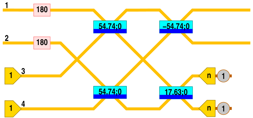
Figure 1: Optical network realizing $\mathsf{CS}_{180^{\circ}}$. The notation is as explained in knill:qc2000e .

A matrix that can be extended to obtain $\mathsf{CS}_{90^{\circ}}$ by post-selection was also obtained:

$$V_{90^{\circ}}=\left(\begin{array}[]{@{}llll@{}}-0.3202+0.0418i&-0.2520-0.3226i&0.2883&-0.1292-0.7221i\\ -0.2520-0.3226i&-0.3202+0.0418i&-0.1292-0.7221i&0.2883\\ -0.3216+0.7210i&-0.1711-0.1725i&0.2469&0.3322+0.3285i\\ -0.1711-0.1725i&-0.3216+0.7210i&0.3322+0.3285i&0.2469\end{array}\right)$$ (12)

The probability of success for this solution is $1/19.37$. A “nice” beam splitter decomposition of this matrix was not found. Partly this is due to the fact that because only two of the singular values are (close to) one, at least two extra modes must be added for the unitary completion. The simplest method of decomposing a $6\times 6$ unitary matrix normally requires $15$ beam splitters.

It is an open problem to determine whether the above solutions are indeed optimal as is suggested by the results of the numerical experiments.

IV Bounds on conditional phase shifts?

To obtain bounds on the probability of success of a phase-shift gate implemented with helper photons, one can attempt to characterize the states obtained in the output modes after tracing out the helper modes. There is some choice of the initial state of the modes that the gate is applied to. Assume that this is a state obtained by applying linear optics to prepared single photons. In this case, the final state after a linear optics transformation is given by

$$\mbox{$|||$}{\psi_{f}}\mbox{$\rangle\rangle\rangle$}=\prod_{k=1}^{n}(\alpha_{k1}{{\mathbf{c}}}^{({\mathsf{1}})}+\ldots+\alpha_{km}{{\mathbf{c}}}^{({\mathsf{m}})})\mbox{$|||$}{{\mathbf{0}}}\mbox{$\rangle\rangle\rangle$}.$$ (13)

The goal is to show that after tracing out modes $m^{\prime}+1,\ldots,m$, the state in the remaining modes is a mixture of states of the form

$$\prod_{k=1}^{n}(\beta_{k0}+\beta_{k1}{{\mathbf{c}}}^{({\mathsf{1}})}+\ldots+\beta_{km^{\prime}}{{\mathbf{c}}}^{({\mathsf{m^{\prime}}})})\mbox{$|||$}{{\mathbf{0}}}\mbox{$\rangle\rangle\rangle$}.$$ (14)

In fact, this is the case if the final state before tracing out is also of this form. To be explicit, add to the factors in the expression for $\mbox{$|||$}{\psi_{f}}\mbox{$\rangle\rangle\rangle$}$ any constant terms $\alpha_{k0}$ so that

$$\mbox{$|||$}{\psi_{f}}\mbox{$\rangle\rangle\rangle$}=\prod_{k=1}^{n}(\alpha_{k0}+\alpha_{k1}{{\mathbf{c}}}^{({\mathsf{1}})}+\ldots+\alpha_{km}{{\mathbf{c}}}^{({\mathsf{m}})})\mbox{$|||$}{{\mathbf{0}}}\mbox{$\rangle\rangle\rangle$}.$$ (15)

First trace out mode $\mathsf{m}$. Given an overcomplete set of states $\mbox{$|||$}{\gamma}\mbox{$\rangle\rangle\rangle$}_{{}_{\!\!{\scriptstyle\mathsf{m}}}}$, the state of modes $\mathsf{1}\ldots\mathsf{m}$ is a mixture of the (unnormalized) states ${}^{\scriptstyle\mathsf{m}}\!\mbox{$\langle\langle\langle$}{\gamma}\mbox{$|||$}\mbox{$|||$}{\psi_{f}}\mbox{$\rangle\rangle\rangle$}$. Choosing as the set of states the coherent states and using the fact that for these states ${}^{\scriptstyle\mathsf{m}}\!\mbox{$\langle\langle\langle$}{\gamma}\mbox{$|||$}{{\mathbf{c}}}^{({\mathsf{m}})}={}^{\scriptstyle\mathsf{m}}\!\mbox{$\langle\langle\langle$}{\gamma}\mbox{$|||$}\bar{\gamma}$, the mixture consists of states of the form

$$\prod_{k=1}^{n}(\alpha_{k0}+\bar{\gamma}\alpha_{km}+\alpha_{k1}{{\mathbf{c}}}^{({\mathsf{1}})}+\ldots+\alpha_{k(m-1)}{{\mathbf{c}}}^{({\mathsf{m-1}})})\mbox{$|||$}{{\mathbf{0}}}\mbox{$\rangle\rangle\rangle$}_{{}_{\!\!{\scriptstyle\mathsf{1\ldots(m-1)}}}}.$$ (16)

Iterating this procedure proves the desired result.

Consider the conditional sign-flip gate. With this gate and using a few beam splitters, one can map the state $\mbox{$|||$}{1100}\mbox{$\rangle\rangle\rangle$}$ to the state ${1\over\sqrt{2}}(\mbox{$|||$}{1100}\mbox{$\rangle\rangle\rangle$}+\mbox{$|||$}{0011}\mbox{$\rangle\rangle\rangle$})={1\over\sqrt{2}}({{\mathbf{c}}}^{({\mathsf{1}})}{{\mathbf{c}}}^{({\mathsf{2}})}+{{\mathbf{c}}}^{({\mathsf{3}})}{{\mathbf{c}}}^{({\mathsf{4}})})$, a well-known entangled photon state. By the above, before post-selection on a measurement of the other modes and with $n$ helper photons, the state can be written as a mixture of products of linear expressions in the creation operators. To obtain a bound on the probability of success, it suffices to obtain a bound for the overlap of (normalized) such states with the Bell state. Because the normalized overlap of $({{\mathbf{c}}}^{({\mathsf{1}})}+{{\mathbf{c}}}^{({\mathsf{3}})})({{\mathbf{c}}}^{({\mathsf{2}})}+{{\mathbf{c}}}^{({\mathsf{4}})})$ with the Bell state is $1/\sqrt{2}$, the bound on the probability of success thus obtained can be no smaller than $1/2$. It is clear that the probability of success cannot be made equal to one: The polynomial $xy+uv$ associated with the creation operators in the Bell state cannot be factored.

A problem suggested by the above is:

Problem. What is the maximum probability of success for implementing $\mathsf{CS}_{\theta}$ using linear optics with at most $k$ independently prepared helper photons and post-selection from photon counters without feedback?

It was shown that for $\theta=180^{\circ}$, a probability of success of one is not possible, but for $k\geq 2$, $1/13.5$ can be realized. A variant of the problem asks the same question for conditional sign shifts of two bosonic qubits (a four mode operation). Other directions for investigation are to determine what improvements are possible if active linear optics operations can be used, or if initial states such as prepared entangled photon pairs pittman:qc2001a or photon number states like $\mbox{$|||$}{2}\mbox{$\rangle\rangle\rangle$}$ are available.

Acknowledgements. This work was partially supported by the NSA and the DOE (contract W-7405-ENG-36).

Appendix A Mathematica Notes for Solving Eq. 6–8

The following gives a sequence of steps using Mathematica for solving Eq. 6–8.

(* The columns of V as polynomials of the creation operators
 * c1,c2,c3,c4  with the scaling simplifications. *)
p1 = (v11*c1+v21*c2+v31*c3+v41*c4);
p2 = (v12*c1+v22*c2+v32*c3+v42*c4);
p3 = (c1+v23*c2+c3+c4);
p4 = (v14*c1+c2+v34*c3+c4);

(* The amplitudes that occur in the equations to be solved are: *)

a0000 := Coefficient[p3*p4, c3*c4];
a1010 := Coefficient[p1*p3*p4, c3*c4*c1];
a1001 := Coefficient[p1*p3*p4, c3*c4*c2];
a0110 := Coefficient[p2*p3*p4, c3*c4*c1];
a0101 := Coefficient[p2*p3*p4, c3*c4*c2];
a1111 := Coefficient[p1*p2*p3*p4, c1*c2*c3*c4];
a1120 := Coefficient[p1*p2*p3*p4, c1^2*c3*c4];
a1102 := Coefficient[p1*p2*p3*p4, c2^2*c3*c4];

(* First solve a1001==0.
 * a1001 is linear in the coefficients of p1. *)
p1x34 = Coefficient[a1001, v21];
p1x24 = Coefficient[a1001, v31];
p1x23 = Coefficient[a1001, v41];
(* Parametrize the linear solutions by hand, introducing l12,l13,l14: *)
rl1 = {v21->l12*p1x24 + l13*p1x23,
       v31->l12*(-p1x34) + l14*p1x23,
       v41->l13*(-p1x34) + l14*(-p1x24)};
p1 = p1/.rl1;

(* Similarly for a0110==0. *)
p1x34 = Coefficient[a0110, v12];
p1x24 = Coefficient[a0110, v32];
p1x23 = Coefficient[a0110, v42];
rl2 = {v12->l21*p1x24 + l23*p1x23,
       v32->l21*(-p1x34) + l24*p1x23,
       v42->l23*(-p1x34) + l24*(-p1x24)};
p2 = p2/.rl2;

(* Next solve a1010==a0101==a0000:
 * Again this leads to linear equations in v11 and v22 respectively. *)
x1 = Coefficient[a1010,v11];
ap1010 = Simplify[a1010-x1*v11];
rl3 = {v11->(a0000-ap1010)/x1};
p1 = p1/.rl3;

x2 = Coefficient[a0101,v22];
ap0101 = Simplify[a0101-x2*v22];
rl4 = {v22->(a0000-ap0101)/x2};
p2 = p2/.rl4;

(* Now solve for a1120==0 and a1102==0.
 * This leads to quadratic equations in l12 and l21.
 * Explicitly: *)

ll11 = Coefficient[FullSimplify[a1120],l12*l21];
tl1120 = a1120-ll11*l12*l21;
ll01 = Coefficient[tl1120,l21];
ll10 = Coefficient[tl1120,l12];
ll00 = FullSimplify[tl1120-ll01*l21-ll10*l12];

lm11 = Coefficient[FullSimplify[a1102],l12*l21];
tl1102 = a1102-lm11*l12*l21;
lm01 = Coefficient[tl1102,l21];
lm10 = Coefficient[tl1102,l12];
lm00 = FullSimplify[tl1102-lm01*l21-lm10*l12];

xysols = Solve[x*y*ll11 + x*ll10 + y*ll01 + ll00 == 0 &&
      x*y*lm11 + x*lm10 + y*lm01 + lm00 == 0, {x,y}];
xy1 = FullSimplify[xysols[[1]]];

p1 = (p1/.{l12->x,l21->y})/.xy1;
p2 = (p2/.{l12->x,l21->y})/.xy1;

(*
 * One can now simplify the expressions by removing
 * redundant variables introduced earlier. p1’s coefficients
 * are a function of Coefficient[p1,c4] and similarly for
 * p2. *)
lsimrule = {l13->(l1-l14*(1+v23))/(1+v34),
            l23->(l2-l24*(1+v14))/(1+v34)};
p1 = p1/.lsimrule;
p2 = p2/.lsimrule;
(* Check the identities by evaluating:
 * Answers included after the expression:
FullSimplify[a0000]//InputForm
  1 + v34
FullSimplify[a0101]//InputForm
  1 + v34
FullSimplify[a1010]//InputForm
  1 + v34
FullSimplify[a0110]//InputForm
  0
FullSimplify[a1001]//InputForm
  0
FullSimplify[a1102]//InputForm
  0
FullSimplify[a1120]//InputForm
  0
FullSimplify[a1111]//InputForm
  (-1 - 4*l1*l2*v23^2*v14^2*(-1 + v34)*v34 +
  v34*(-1 - 4*l1*l2*(-1 + v34) + v34 + v34^2 + 2*v23*(1 + v34)^2) +
  v14*(-2*(1 + v34)^2 + v23*(-1 + v34)*(1 + v34*(2 + 8*l1*l2 + v34))))/
 ((1 + v34)*(-1 - (2 + v23)*v14 + v34 + v23*(2 + v14)*v34))
*)

(* Remaining identity: a1111 = ph*a0000, where ph is the desired phase.
 * Note that a1111 is now a function of l1*l2, so solve for that. *)
l1rls = Solve[FullSimplify[a1111 == ph*a0000], {l1}];
l1rl = FullSimplify[l1rls[[1]]];
l1tl2 = l1*l2/.l1rl;

(*
 * Checking shows that p1-c1 and p2-c2 are multiples
 * of l1 and l2 respectively. Exploit that to express
 * the coefficients of p1 and p2: *)
dp1c1 = FullSimplify[(Coefficient[p1,c1]-1)/l1];
dp1c2 = FullSimplify[Coefficient[p1,c2]/l1];
dp1c3 = FullSimplify[Coefficient[p1,c3]/l1];
dp1c4 = FullSimplify[Coefficient[p1,c4]/l1];

dp2c1 = FullSimplify[Coefficient[p2,c1]/l2];
dp2c2 = FullSimplify[(Coefficient[p2,c2]-1)/l2];
dp2c3 = FullSimplify[Coefficient[p2,c3]/l2];
dp2c4 = FullSimplify[Coefficient[p2,c4]/l2];

(* The transpose of V is now given by:
*)
vmat = {{dp1c1,dp1c2,dp1c3,dp1c4}*l1+{1,0,0,0},
        {dp2c1,dp2c2,dp2c3,dp2c4}*l2+{0,1,0,0},
        {1,v23, 1, 1},
        {v14,1,v34,1}};
(* Formulas:
dp1c1//InputForm
(1 + v14 + v23*v14 - 2*v14^2 - v23*v14^2 - 2*v34 + 2*v23*v34 - 4*v14*v34 +
  4*v23*v14*v34 - 2*v14^2*v34 + 2*v23*v14^2*v34 + v34^2 + 2*v23*v34^2 -
  v14*v34^2 - v23*v14*v34^2 - v23*v14^2*v34^2 +
  (1 + v14)*Sqrt[v14^2*(v23*(-1 + v34)^2 + 2*(1 + v34))^2 +
     2*v14*(2*(-1 + v34)^2*(1 + v34) + 2*v23^2*(-1 + v34)^2*v34*(1 + v34) +
       v23*(1 - 18*v34^2 + v34^4)) + (1 + v34*(-2 + v34 + 2*v23*(1 + v34)))^
      2])/(2*(1 + v34)*(-1 - (2 + v23)*v14 + v34 + v23*(2 + v14)*v34))
dp1c2//InputForm
(-1 + v23 - 2*v14 + v23*v14 + v23^2*v14 + 2*v34 + 4*v23*v34 + 2*v23^2*v34 -
  2*v14*v34 - 4*v23*v14*v34 - 2*v23^2*v14*v34 - v34^2 - v23*v34^2 +
  2*v23^2*v34^2 - v23*v14*v34^2 + v23^2*v14*v34^2 +
  (1 + v23)*Sqrt[v14^2*(v23*(-1 + v34)^2 + 2*(1 + v34))^2 +
     2*v14*(2*(-1 + v34)^2*(1 + v34) + 2*v23^2*(-1 + v34)^2*v34*(1 + v34) +
       v23*(1 - 18*v34^2 + v34^4)) + (1 + v34*(-2 + v34 + 2*v23*(1 + v34)))^
      2])/(2*(1 + v34)*(-1 - (2 + v23)*v14 + v34 + v23*(2 + v14)*v34))
dp1c3//InputForm
((-1 + v34)*(1 + (2 + v23)*v14 + v34 + v23*(2 + v14)*v34) -
  Sqrt[v14^2*(v23*(-1 + v34)^2 + 2*(1 + v34))^2 +
    2*v14*(2*(-1 + v34)^2*(1 + v34) + 2*v23^2*(-1 + v34)^2*v34*(1 + v34) +
      v23*(1 - 18*v34^2 + v34^4)) + (1 + v34*(-2 + v34 + 2*v23*(1 + v34)))^
     2])/(2*(-1 - (2 + v23)*v14 + v34 + v23*(2 + v14)*v34))
dp1c4//InputForm
 -1
dp2c1//InputForm
(1 + v14 + v23*v14 - 2*v14^2 - v23*v14^2 - 2*v34 + 2*v23*v34 - 4*v14*v34 +
  4*v23*v14*v34 - 2*v14^2*v34 + 2*v23*v14^2*v34 + v34^2 + 2*v23*v34^2 -
  v14*v34^2 - v23*v14*v34^2 - v23*v14^2*v34^2 -
  (1 + v14)*Sqrt[v14^2*(v23*(-1 + v34)^2 + 2*(1 + v34))^2 +
     2*v14*(2*(-1 + v34)^2*(1 + v34) + 2*v23^2*(-1 + v34)^2*v34*(1 + v34) +
       v23*(1 - 18*v34^2 + v34^4)) + (1 + v34*(-2 + v34 + 2*v23*(1 + v34)))^
      2])/(2*(1 + v34)*(-1 - (2 + v23)*v14 + v34 + v23*(2 + v14)*v34))
dp2c2//InputForm
(-1 + v23 - 2*v14 + v23*v14 + v23^2*v14 + 2*v34 + 4*v23*v34 + 2*v23^2*v34 -
  2*v14*v34 - 4*v23*v14*v34 - 2*v23^2*v14*v34 - v34^2 - v23*v34^2 +
  2*v23^2*v34^2 - v23*v14*v34^2 + v23^2*v14*v34^2 -
  (1 + v23)*Sqrt[v14^2*(v23*(-1 + v34)^2 + 2*(1 + v34))^2 +
     2*v14*(2*(-1 + v34)^2*(1 + v34) + 2*v23^2*(-1 + v34)^2*v34*(1 + v34) +
       v23*(1 - 18*v34^2 + v34^4)) + (1 + v34*(-2 + v34 + 2*v23*(1 + v34)))^
      2])/(2*(1 + v34)*(-1 - (2 + v23)*v14 + v34 + v23*(2 + v14)*v34))
dp2c3//InputForm
((-1 + v34)*(1 + (2 + v23)*v14 + v34 + v23*(2 + v14)*v34) +
  Sqrt[v14^2*(v23*(-1 + v34)^2 + 2*(1 + v34))^2 +
    2*v14*(2*(-1 + v34)^2*(1 + v34) + 2*v23^2*(-1 + v34)^2*v34*(1 + v34) +
      v23*(1 - 18*v34^2 + v34^4)) + (1 + v34*(-2 + v34 + 2*v23*(1 + v34)))^
     2])/(2*(-1 - (2 + v23)*v14 + v34 + v23*(2 + v14)*v34))
dp2c4//InputForm
-1
* And l1*l2 ==
l1tl2//InputForm
  -((-1 + ph)*(1 + v34)^2*(-1 - (2 + v23)*v14 + v34 + v23*(2 + v14)*v34))/
   (4*(-1 + v23*v14)^2*(-1 + v34)*v34)
*)

References

- [1] E. Knill, R. Laflamme, and G. Milburn. A scheme for efficient linear optics quantum computation. Nature, 409:46–52, 2001.
- [2] D. Gottesman, A. Kitaev, and J. Preskill. Encoding a qudit in an oscillator. Phys. Rev. A, 64:012310/1–21, 2001.
- [3] T. C. Ralph, W. J. Munro, and G. J. Milburn. Quantum computation with coherent states, linear interactions and superposed resources. quant-ph/0110115, 2001.
- [4] T.C.Ralph, A.G.White, W.J.Munro, and G.J.Milburn. Simple scheme for efficient linear optics quantum gates. quant-ph/0108049, 2001.
- [5] T. Rudolph and J.-W. Pan. A simple gate for linear optics quantum computing. quant-ph/0108056, 2001.
- [6] T. B. Pittman, B. C. Jacobs, and J. D. Franson. Probabilistic quantum logic operations using polarizing beam splitters. quant-ph/0107091, 2001.
- [7] T. B. Pittman, B. C. Jacobs, and J. D. Franson. Demonstration of non-deterministic quantum logic operations using linear optical elements. quant-ph/0109128, 2001.
- [8] N. Lütkenhaus, J. Calsamiglia, and K.-A. Suominen. Bell measurements for teleportation. Phys. Rev. A, 59:3295–3300, 1999.
- [9] J. Calsamiglia. Generalized measurements by linear elements. quant-ph/0108108, 2001.
- [10] M. Reck, A. Zeilinger, H. J. Bernstein, and P. Bertani. Experimental realization of a discrete unitary operator. Phys. Rev. Lett., 73:58–61, 1994.