[

Efficient quantum computation of high harmonics of the Liouville density distribution

Abstract

We show explicitly that high harmonics of the classical Liouville density distribution in the chaotic régime can be obtained efficiently on a quantum computer [1, 2]. As was stated in [1], this provides information unaccessible for classical computer simulations, and replies to the questions raised in [3, 4].

]

In our Letter [1] we showed on the example of Arnold cat map that classical chaotic dynamics of exponentially many orbits can be simulated in polynomial time on a quantum computer. The Liouville density distribution $P(x_{i},y_{j})$ is encoded on a discretized lattice ($2^{n_{q}}\times 2^{n_{q}}$) using $3n_{q}-1$ qubits organized in three registers. After each map iteration, the distribution is coded in the quantum state $\sum_{i,j}a_{ij}|x_{i}>|y_{j}>|0>$ with $P(x_{i},y_{j})=a_{ij}$ and $x_{i}=i/N$, $y_{j}=j/N$, $N=2^{n_{q}}$ [5]. One measurement of qubits in this basis gives one point in the phase space and therefore the distribution $P(x_{i},y_{j})$ can be obtained approximately in polynomial number of measurements. However the same information can be obtained via classical Monte Carlo simulation with a polynomial number of orbits, as it was discussed by us in [2] and later repeated in [3]. Based on this observation, the comment [3] makes a general claim that no new information can be extracted efficiently from quantum computation of such classical maps (paragraph 3 in [3]) (see also the comment [4]). Here we show that this statement is incorrect. Indeed, the quantum Fourier transform (QFT) of $a_{ij}$ provides nondiagonal observables [1], namely the Fourier components $\tilde{P}(k_{x},k_{y})=\sum_{i,j}\exp(i2\pi(k_{x}x_{i}+k_{y}y_{j}))a_{ij}/N$. They obviously contain important information relevant for the classical dynamics, and require $O(n_{q}^{2})$ operations including measurement. On the contrary, all known classical algorithms will require exponential number of operations to obtain correct probabilities at high harmonics $k_{x,y}\sim N$. Such harmonics are important since due to chaos a significant part of total probability is transfered to wavevectors with $k\sim\exp(ht)$ where $h$ is the Kolmogorov-Sinai entropy, and $t$ is the number of iterations (see [6]). We note that the claim of [3] applies equally to the Shor algorithm, where all information is also encoded only in squared moduli of amplitudes, but where the QFT produces classically unaccessible information.

In Fig.1 we present the probability $\tilde{P}(k_{x},k_{y})$ in Fourier space for different times $t$. We note that a 2-dimensional (2d) QFT can be efficiently implemented by application of usual QFT to each register consecutively. The results show that $\tilde{P}$ is composed of well-pronounced peaks, most of which move with time to high wavevectors $k$. They remain stable in presence of noise in the quantum gates (e.g. top right panel in Fig.1 is unchanged if $1\%$ noise is added in each gate). The location and amplitude of these peaks can be extracted from a polynomial number of measurements of qubits after the 2d QFT.

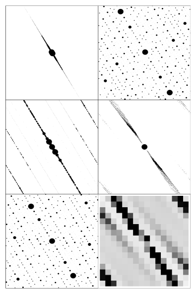
FIG. 1.: Fourier coefficients $|\tilde{P}(k_{x},k_{y})|^{2}$ of Liouville distribution for $-N/2\leq k_{x,y}\leq N/2$, initial state as in Fig.1 of $[1]$. Left column: cat map at $t=3,5,7$ from top to bottom for $n_{q}=10$. Top right: same at $t=5$, $n_{q}=7$. Middle right: $|\tilde{P}(k_{x},k_{y})|^{2}$ for perturbed cat map (see text) at $t=5$, $n_{q}=10$. Peaks are shown by circles; maximal circle size marks peaks with $1>|\tilde{P}(k_{x},k_{y})|^{2}>0.1$, circles twice smaller those with $0.1>|\tilde{P}(k_{x},k_{y})|^{2}>0.01$, etc… Bottom right: coarse-grained image of $|\tilde{P}(k_{x},k_{y})|^{2}$ (proportional to grayness) for the data of middle right panel, $n_{f}=4$.

For the Arnold cat map the dynamics in $(k_{x},k_{y})$ space is especially simple, given by $\bar{k_{x}}=k_{x}-k_{y},\;\bar{k_{y}}=2k_{y}-k_{x}\;\mbox{(mod}\;\mbox{N)}$. However, generally this dynamics is very complicated. To exemplify this, we simulated the perturbed cat map $\bar{y}=y+x+x^{2},\;\bar{x}=x+\bar{y}\;\mbox{(mod}\;\mbox{1)}$ (Fig. 1). It can be iterated in $O(n_{q}^{2})$ operations on a quantum computer using modular multiplication. In this case, main peaks can be seen directly for short times, while for larger times a polynomial number of measurements of the first $n_{f}$ qubits [2] gives a coarse-grained image of $|\tilde{P}(k_{x},k_{y})|^{2}$, including very high harmonics, which are unaccessible to classical computation [7].

As concerns the issue of errors in the computation, raised in [4], it should be stressed that the main aim of [1] was to compare the errors natural for classical and quantum computers. In fact, we showed that the natural/minimal (last bit) errors for classical computer grow exponentially with number of map iterations while the natural errors in quantum gates do not destroy the time reversibility (Fig. 1 of [1]). As a further example, Fig. 1 of [8] clearly shows that the errors of relative precision $10^{-8}$ (comparable with ordinary precision on Pentium III) completely destroy the reversibility of classical dynamics. At the same time, the quantum errors of relative precision $10^{-2}$ in operations of quantum gates preserve the reversibility. Of course, since the quantum algorithm simulates the classical discretized map exactly, the last bit errors made on a quantum computer lead to exponential divergence of nearby trajectories and exponential drop of fidelity. This is clearly illustrated by Fig. 3 in [1]. Thus exponential instability of classical chaos is preserved in quantum simulations. The quantum computer has enormous capacity in memory and precision which grows exponentially with the number of qubits; thus in the quantum case the last bit errors are much less important than for the classical computer with its limited memory space. However, the quantum computer has its own natural errors related to imperfections in gate operations. The results presented in [1, 2, 8] show that the quantum simulation is stable with respect to its natural errors in quantum gates operations while the classical computation is unstable with respect to its natural errors in the last bit of dynamical variables.

This work was supported in part by the NSA and ARDA under ARO contract number DAAD19-01-1-0553.

REFERENCES

- [1] B. Georgeot and D. L. Shepelyansky, Phys. Rev. Lett 86 5393 (2001), quant-ph/0101004.
- [2] B. Georgeot and D. L. Shepelyansky, quant-ph/0102082v2.
- [3] L. Diosi, quant-ph/0110026.
- [4] C. Zalka, quant-ph/0110019.
- [5] An initial distribution with exponentially many orbits can be prepared efficiently on a quantum computer; for example a square of size can be built by using Hadamard gates acting on the last qubits of each register .
- [6] A. Lichtenberg and M. Lieberman, Regular and Chaotic Dynamics, Springer, N.Y. (1992).
- [7] Contrary to what was argued in [4], high harmonics cannot be found from the fine structure of “a few closely spaced final points”, since the Fourier coefficients involve the full distribution.
- [8] B. Georgeot and D. L. Shepelyansky, quant-ph/0105149.