On the concepts of radial and angular kinetic energies

Abstract

We consider a general central-field system in $D$ dimensions and show that the division of the kinetic energy into radial and angular parts proceeds differently in the wavefunction picture and the Weyl-Wigner phase-space picture. Thus, the radial and angular kinetic energies are different quantities in the two pictures, containing different physical information, but the relation between them is well defined. We discuss this relation and illustrate its nature by examples referring to a free-particle and to a ground-state hydrogen atom.

I Introduction

Phase-space representations of quantum mechanics play an increasingly important role in several branches of physics, including quantum optics and atomic physics. The principal reason for this is the conceptual possibility these representations give for viewing the position and momentum characteristics of a quantum state in the same picture. Phase space is often useful for the description of stationary states, and it has become a natural background for describing the quantum-mechanical time evolution of wavepackets, for both matter waves and electromagnetic waves. Several phase-space representations have been discussed in the literature, but one of them—the so-called Weyl-Wigner representation—has come to play the role of a canonical phase-space representation, because of its simplicity [1, 2]. In accordance with this, we shall exclusively consider the Weyl-Wigner representation in the following.

We consider this phase-space representation to be a representation in its own right. In previous work [3, 4, 5] we have justified this statement by analyzing and solving the phase-space differential equations that the Wigner functions must satisfy. In particular, we have stressed that the Wigner functions may be determined directly from these equations, without reference to wavefunctions—although it is in general easier to determine them from the wavefunctions.

The fact that the phase-space description is a representation in its own right makes it relevant to apply physical intuition to the form and behavior of the Wigner functions, just as physical intuition may be applied to the form and behavior of wavefunctions. When we do this, we discover that our understanding of quantum states becomes enlarged, because the two types of intuition may work differently and therefore supplement each other.

In the present investigation which, for the sake of generality, is carried out in $D$ dimensions, we consider quantum states referred to a center $O$. We focus, in particular, on the evaluation of the angular momentum and the kinetic energy of such states. In the familiar picture based on wavefunctions, these quantities are calculated as the expectation values of operators. In the phase-space picture they are calculated by taking averages of dynamical phase-space functions with Wigner distribution functions. Performing the two calculations with care will, of course, lead to the same result. Yet, a comparison between the detailed features of the two descriptions leads to some interesting and physically important observations.

This was already noted in our previous work on the Wigner function for the ground state of the hydrogen atom [6], in which we touched on a pedagogical dilemma which, for instance, has bothered writers of elementary textbooks [7]: How does one bring the fact that the angular momentum in the Bohr orbit is non-zero into accordance with the fact that the angular momentum in the Schrödinger picture is zero? We referred to this dilemma as the angular-momentum dilemma and showed that it could be resolved by noting that the mapping of the operator $\hat{L}^{2}$ to phase space produces the phase-space function $|\mathchoice{{\hbox{\boldmath$\displaystyle r$}}}{{\hbox{\boldmath$\textstyle r$}}}{{\hbox{\boldmath$\scriptstyle r$}}}{{\hbox{\boldmath$\scriptscriptstyle r$}}}\times\mathchoice{{\hbox{\boldmath$\displaystyle p$}}}{{\hbox{\boldmath$\textstyle p$}}}{{\hbox{\boldmath$\scriptstyle p$}}}{{\hbox{\boldmath$\scriptscriptstyle p$}}}|^{2}-3\hbar^{2}/2$ rather than just $|\mathchoice{{\hbox{\boldmath$\displaystyle r$}}}{{\hbox{\boldmath$\textstyle r$}}}{{\hbox{\boldmath$\scriptstyle r$}}}{{\hbox{\boldmath$\scriptscriptstyle r$}}}\times\mathchoice{{\hbox{\boldmath$\displaystyle p$}}}{{\hbox{\boldmath$\textstyle p$}}}{{\hbox{\boldmath$\scriptstyle p$}}}{{\hbox{\boldmath$\scriptscriptstyle p$}}}|^{2}$.

In the following, we generalize this result to $D$ dimensions. In addition, we derive parallel but more faceted relations for kinetic-energy quantities, likewise in $D$ dimensions. We discuss these results and show that the separation of kinetic energy into a radial and an angular part may be done in two physically meaningful ways. One is suggested by the form of the operators in the wave-function picture, the other by classical-like dynamical functions in the phase-space picture. The relation between the two variants of radial and angular kinetic energies is tied to the Weyl correspondence rule and is, therefore, well defined.

We illustrate the conceptual difference between the two types of kinetic-energy separation by two important examples in three dimensions. One is the simplest possible time-dependent state of a free particle, the other is the stationary ground state of the hydrogen atom. For the first example, we find that the phase-space induced separation of the kinetic energy into a radial and an angular part depends on time in an intuitively simple way, whereas the operator-based separation is independent of time. For the ground state of the hydrogen atom, the operator-based separation leads to an angular kinetic energy of zero, whereas the phase-space induced separation classifies the whole kinetic energy as angular kinetic energy. This striking difference between the results of the two types of separation is well reflected in the form of the wavefunction versus the form of the Wigner function. It illustrates in a perfect way how the physical richness that is hidden in the simplest state of the simplest atom can only be seen by looking at the state from different angles. It also illustrates the intricate way in which the roots of classical mechanics are buried in the quantum-mechanical soil.

The paper, which is intended to be reasonably self contained, is organized in the following way: In Sec. II we give a brief overview of hyperspherical coordinates and the central-field form of wavefunctions in $D$ dimensions. In Sec. III we define the angular momentum and perform the operator-based separation of the kinetic energy into a radial and an angular part. We express the result both in terms of general operators and in terms of differential operators. As a background for the rest of the paper we recall the salient aspects of the Weyl-Wigner transformation in Sec. IV . In Sec. V we discuss the concept of angular momentum in the phase-space picture. We introduce the concepts of $q$ (quantum) angular momentum and $c$ (classical-like) angular momentum and discuss the relation between them. In Sec. VI we give a similar discussion of the kinetic energy in phase space and of its separation into a radial part and an angular part. Secs. VII and VIII are devoted to two illustrative examples in three dimensions. Sec. IX generalizes the examples to $D$ dimensions. Sec. X is our conclusion.

II Hyperspherical Coordinates

Let $\mathchoice{{\hbox{\boldmath$\displaystyle r$}}}{{\hbox{\boldmath$\textstyle r$}}}{{\hbox{\boldmath$\scriptstyle r$}}}{{\hbox{\boldmath$\scriptscriptstyle r$}}}=(x_{1},x_{2},\ldots,x_{D})$ be the position vector of a ‘particle’ moving in $D$-dimensional position space [8], and let $\mathchoice{{\hbox{\boldmath$\displaystyle p$}}}{{\hbox{\boldmath$\textstyle p$}}}{{\hbox{\boldmath$\scriptstyle p$}}}{{\hbox{\boldmath$\scriptscriptstyle p$}}}=(p_{1},p_{2},\ldots,p_{D})$ be its conjugate momentum. We take $x_{i}$, and hence also $p_{i}$, to be Cartesian coordinates. In accordance with this, we introduce the hyperradius $r$ by the relation $r^{2}=x_{1}^{2}+x_{2}^{2}+\ldots+x_{D}^{2}$, and likewise $p$, the magnitude of the momentum, by the relation $p^{2}=p_{1}^{2}+p_{2}^{2}+\ldots+p_{D}^{2}$. Quantum mechanically, we adopt the position-space representation and write

$$\hat{\mathchoice{{\hbox{\boldmath$\displaystyle p$}}}{{\hbox{\boldmath$\textstyle p$}}}{{\hbox{\boldmath$\scriptstyle p$}}}{{\hbox{\boldmath$\scriptscriptstyle p$}}}}=(\hat{p}_{1},\hat{p}_{2},\ldots,\hat{p}_{D})=-i\hbar\left(\frac{\partial}{\partial x_{1}},\frac{\partial}{\partial x_{2}},\ldots,\frac{\partial}{\partial x_{D}}\right),$$ (1)

and

$$\hat{p}^{2}=-\hbar^{2}\left(\frac{\partial^{2}}{\partial x_{1}^{2}}+\frac{\partial^{2}}{\partial x_{2}^{2}}+\ldots+\frac{\partial^{2}}{\partial x_{D}^{2}}\right)=-\hbar^{2}\nabla^{2},$$ (2)

where $\nabla^{2}$ is the $D$-dimensional Laplacian. The kinetic energy of a quantum-mechanical particle with mass $M$ is represented by the operator

$$\hat{T}=\frac{\hat{p}^{2}}{2M}=-\frac{\hbar^{2}}{2M}\nabla^{2}\,.$$ (3)

The central-field Hamiltonian

$$\hat{H}=\frac{\hat{p}^{2}}{2M}+V(r)$$ (4)

determines the motion of the particle in a central field $V(r)$.

To introduce hyperspherical coordinates in position space, one writes $x_{i}=r\eta_{i}$, where the $\eta_{i}$’s are $D$ functions of $D-1$ angular coordinates. Both the angles and the $\eta_{i}$’s may be chosen in different ways, but a choice similar to the following one is generally used, albeit with varying notation for the angles:

$$x_{1} = r\sin\theta_{D-1}\sin\theta_{D-2}\ldots\sin\theta_{2}\sin\theta_{1}$$ (5)

$$x_{2} = r\sin\theta_{D-1}\sin\theta_{D-2}\ldots\sin\theta_{2}\cos\theta_{1}$$ (6)

$$x_{3} = r\sin\theta_{D-1}\sin\theta_{D-2}\ldots\cos\theta_{2}$$ (7)

$$\vdots$$ (8)

$$x_{D-1} = r\sin\theta_{D-1}\cos\theta_{D-2}$$ (9)

$$x_{D} = r\cos\theta_{D-1}$$ (10)

with ($0\leq r\leq\infty$), ($0\leq\theta_{1}<2\pi$), ($0\leq\theta_{2}<\pi$), …, ($0\leq\theta_{D-1}<\pi$). A similar representation may, of course, be set up for the vector $\textstyle p$ in momentum space.

For the volume element in position space we have the expression

$$d\mathchoice{{\hbox{\boldmath$\displaystyle r$}}}{{\hbox{\boldmath$\textstyle r$}}}{{\hbox{\boldmath$\scriptstyle r$}}}{{\hbox{\boldmath$\scriptscriptstyle r$}}}=dx_{1}dx_{2}\ldots dx_{D}=r^{D-1}drd\Omega,$$ (11)

where the solid-angle element $d\Omega$ is given by

$$d\Omega = (\sin\theta_{D-1})^{D-2}(\sin\theta_{D-2})^{D-3}\ldots\sin\theta_{2}$$ (13)

$$\times d\theta_{D-1}\ldots d\theta_{2}d\theta_{1}.$$

Integrating over all angles gives the total solid angle:

$$S_{D}=\int d\Omega=\frac{2\pi^{D/2}}{\Gamma(D/2)}\,.$$ (14)

Wavefunctions of the central-field problem are conveniently referred to basis functions of the form

$$\psi(\mathchoice{{\hbox{\boldmath$\displaystyle r$}}}{{\hbox{\boldmath$\textstyle r$}}}{{\hbox{\boldmath$\scriptstyle r$}}}{{\hbox{\boldmath$\scriptscriptstyle r$}}})=R(r)Y(\Omega)$$ (15)

where $\Omega$ is a collective notation for the angular coordinates $(\theta_{1},\theta_{2},\ldots,\theta_{D-1})$, and $Y(\Omega)$ is a hyperspherical harmonic. The hyperspherical harmonics were introduced and extensively studied by Green [9] and Hill [10]. They have also been much studied by later authors. (See, in particular, the comprehensive presentations by Sommerfeld [11], Louck [12] and Avery [13].) The hyperspherical harmonics are eigenfunctions of the operator $\hat{L}^{2}$ which represents the square of the total angular momentum and is defined below.

III Angular Momentum and Kinetic Energy

The angular-momentum tensor in $D$ dimensions is defined by the operators

$$\hat{L}_{ij}=x_{i}\hat{p}_{j}-x_{j}\hat{p}_{i},\qquad i\neq j.$$ (16)

The square of the total angular momentum is

$$\hat{L}^{2}=\frac{1}{2}\sum_{i=1}^{D}{\sum_{j=1}^{D}}{}^{\prime}\hat{L}_{ij}^{2},$$ (17)

where the prime indicates that the double sum excludes terms for which $i=j$. The angular-momentum operators are independent of $r$. They merely depend upon the angular coordinates.

We shall now separate the kinetic-energy operator $\hat{T}$ into two distinctive parts. To accomplish this in a manner that eases the subsequent transition to the phase-space representation, we begin by decomposing the $D$-dimensional unit matrix $\textstyle 1$ as follows:

$$\mathchoice{{\hbox{\boldmath$\displaystyle 1$}}}{{\hbox{\boldmath$\textstyle 1$}}}{{\hbox{\boldmath$\scriptstyle 1$}}}{{\hbox{\boldmath$\scriptscriptstyle 1$}}}=\frac{\mathchoice{{\hbox{\boldmath$\displaystyle S$}}}{{\hbox{\boldmath$\textstyle S$}}}{{\hbox{\boldmath$\scriptstyle S$}}}{{\hbox{\boldmath$\scriptscriptstyle S$}}}}{r^{2}}+\frac{1}{2}\sum_{i=1}^{D}{\sum_{j=1}^{D}}{}^{\prime}\frac{\mathchoice{{\hbox{\boldmath$\displaystyle T$}}}{{\hbox{\boldmath$\textstyle T$}}}{{\hbox{\boldmath$\scriptstyle T$}}}{{\hbox{\boldmath$\scriptscriptstyle T$}}}^{ij}}{r^{2}}\,.$$ (18)

The matrices $\textstyle S$ and $\mathchoice{{\hbox{\boldmath$\displaystyle T$}}}{{\hbox{\boldmath$\textstyle T$}}}{{\hbox{\boldmath$\scriptstyle T$}}}{{\hbox{\boldmath$\scriptscriptstyle T$}}}^{ij}$ are defined by the relations

$$S_{kl}=x_{k}x_{l}$$ (19)

and

$$(\mathchoice{{\hbox{\boldmath$\displaystyle T$}}}{{\hbox{\boldmath$\textstyle T$}}}{{\hbox{\boldmath$\scriptstyle T$}}}{{\hbox{\boldmath$\scriptscriptstyle T$}}}^{ij})_{kl} = x_{i}^{2}\delta_{kj}\delta_{lj}+x_{j}^{2}\delta_{ki}\delta_{li}-x_{i}x_{j}(\delta_{ki}\delta_{lj}+\delta_{kj}\delta_{li}),$$ (21)

$$i\neq j,$$

or,

$$\mathchoice{{\hbox{\boldmath$\displaystyle S$}}}{{\hbox{\boldmath$\textstyle S$}}}{{\hbox{\boldmath$\scriptstyle S$}}}{{\hbox{\boldmath$\scriptscriptstyle S$}}}=\left(\begin{array}[]{cccc}x_{1}^{2}&x_{1}x_{2}&\cdots&x_{1}x_{D}\\ x_{2}x_{1}&x_{2}^{2}&\cdots&x_{2}x_{D}\\ \cdot&\cdot&\cdots&\cdot\\ x_{D}x_{1}&x_{D}x_{2}&\cdots&x_{D}^{2}\end{array}\right)$$ (22)

and, for instance,

$$\mathchoice{{\hbox{\boldmath$\displaystyle T$}}}{{\hbox{\boldmath$\textstyle T$}}}{{\hbox{\boldmath$\scriptstyle T$}}}{{\hbox{\boldmath$\scriptscriptstyle T$}}}^{12}=\left(\begin{array}[]{ccccc}x_{2}^{2}&-x_{1}x_{2}&0&\cdots&0\\ -x_{2}x_{1}&x_{1}^{2}&0&\cdots&0\\ 0&0&0&\cdots&0\\ \cdot&\cdot&\cdot&\cdots&\cdot\\ 0&0&0&\cdots&0\end{array}\right)\,.$$ (23)

Adopting a dyadic notation, we may then write

$$\hat{T}=\frac{1}{2M}\hat{\mathchoice{{\hbox{\boldmath$\displaystyle p$}}}{{\hbox{\boldmath$\textstyle p$}}}{{\hbox{\boldmath$\scriptstyle p$}}}{{\hbox{\boldmath$\scriptscriptstyle p$}}}}\cdot\left(\frac{\mathchoice{{\hbox{\boldmath$\displaystyle S$}}}{{\hbox{\boldmath$\textstyle S$}}}{{\hbox{\boldmath$\scriptstyle S$}}}{{\hbox{\boldmath$\scriptscriptstyle S$}}}}{r^{2}}+\frac{1}{2}\sum_{i=1}^{D}{\sum_{j=1}^{D}}{}^{\prime}\frac{\mathchoice{{\hbox{\boldmath$\displaystyle T$}}}{{\hbox{\boldmath$\textstyle T$}}}{{\hbox{\boldmath$\scriptstyle T$}}}{{\hbox{\boldmath$\scriptscriptstyle T$}}}^{ij}}{r^{2}}\right)\cdot\hat{\mathchoice{{\hbox{\boldmath$\displaystyle p$}}}{{\hbox{\boldmath$\textstyle p$}}}{{\hbox{\boldmath$\scriptstyle p$}}}{{\hbox{\boldmath$\scriptscriptstyle p$}}}}\,.$$ (24)

Next, we note that

$$\hat{\mathchoice{{\hbox{\boldmath$\displaystyle p$}}}{{\hbox{\boldmath$\textstyle p$}}}{{\hbox{\boldmath$\scriptstyle p$}}}{{\hbox{\boldmath$\scriptscriptstyle p$}}}}\cdot\frac{\mathchoice{{\hbox{\boldmath$\displaystyle S$}}}{{\hbox{\boldmath$\textstyle S$}}}{{\hbox{\boldmath$\scriptstyle S$}}}{{\hbox{\boldmath$\scriptscriptstyle S$}}}}{r^{2}}\cdot\hat{\mathchoice{{\hbox{\boldmath$\displaystyle p$}}}{{\hbox{\boldmath$\textstyle p$}}}{{\hbox{\boldmath$\scriptstyle p$}}}{{\hbox{\boldmath$\scriptscriptstyle p$}}}}=\left(\hat{\mathchoice{{\hbox{\boldmath$\displaystyle p$}}}{{\hbox{\boldmath$\textstyle p$}}}{{\hbox{\boldmath$\scriptstyle p$}}}{{\hbox{\boldmath$\scriptscriptstyle p$}}}}\cdot\frac{\mathchoice{{\hbox{\boldmath$\displaystyle r$}}}{{\hbox{\boldmath$\textstyle r$}}}{{\hbox{\boldmath$\scriptstyle r$}}}{{\hbox{\boldmath$\scriptscriptstyle r$}}}}{r}\right)\left(\frac{\mathchoice{{\hbox{\boldmath$\displaystyle r$}}}{{\hbox{\boldmath$\textstyle r$}}}{{\hbox{\boldmath$\scriptstyle r$}}}{{\hbox{\boldmath$\scriptscriptstyle r$}}}}{r}\cdot\hat{\mathchoice{{\hbox{\boldmath$\displaystyle p$}}}{{\hbox{\boldmath$\textstyle p$}}}{{\hbox{\boldmath$\scriptstyle p$}}}{{\hbox{\boldmath$\scriptscriptstyle p$}}}}\right)$$ (25)

and

$$\hat{\mathchoice{{\hbox{\boldmath$\displaystyle p$}}}{{\hbox{\boldmath$\textstyle p$}}}{{\hbox{\boldmath$\scriptstyle p$}}}{{\hbox{\boldmath$\scriptscriptstyle p$}}}}\cdot\frac{\mathchoice{{\hbox{\boldmath$\displaystyle T$}}}{{\hbox{\boldmath$\textstyle T$}}}{{\hbox{\boldmath$\scriptstyle T$}}}{{\hbox{\boldmath$\scriptscriptstyle T$}}}^{ij}}{r^{2}}\cdot\hat{\mathchoice{{\hbox{\boldmath$\displaystyle p$}}}{{\hbox{\boldmath$\textstyle p$}}}{{\hbox{\boldmath$\scriptstyle p$}}}{{\hbox{\boldmath$\scriptscriptstyle p$}}}}=\frac{\hat{L}_{ij}^{2}}{r^{2}}\,.$$ (26)

Hence, the kinetic-energy operator may be written

$$\hat{T} = \hat{T}_{rad}+\hat{T}_{ang}$$ (27)

$$= \frac{1}{2M}\left(\hat{\mathchoice{{\hbox{\boldmath$\displaystyle p$}}}{{\hbox{\boldmath$\textstyle p$}}}{{\hbox{\boldmath$\scriptstyle p$}}}{{\hbox{\boldmath$\scriptscriptstyle p$}}}}\cdot\frac{\mathchoice{{\hbox{\boldmath$\displaystyle r$}}}{{\hbox{\boldmath$\textstyle r$}}}{{\hbox{\boldmath$\scriptstyle r$}}}{{\hbox{\boldmath$\scriptscriptstyle r$}}}}{r}\right)\left(\frac{\mathchoice{{\hbox{\boldmath$\displaystyle r$}}}{{\hbox{\boldmath$\textstyle r$}}}{{\hbox{\boldmath$\scriptstyle r$}}}{{\hbox{\boldmath$\scriptscriptstyle r$}}}}{r}\cdot\hat{\mathchoice{{\hbox{\boldmath$\displaystyle p$}}}{{\hbox{\boldmath$\textstyle p$}}}{{\hbox{\boldmath$\scriptstyle p$}}}{{\hbox{\boldmath$\scriptscriptstyle p$}}}}\right)+\frac{\hat{L}^{2}}{2Mr^{2}}\,,$$ (28)

where $\hat{T}_{rad}$ has the form

$$\hat{T}_{rad}=\frac{1}{2M}\left(\hat{\mathchoice{{\hbox{\boldmath$\displaystyle p$}}}{{\hbox{\boldmath$\textstyle p$}}}{{\hbox{\boldmath$\scriptstyle p$}}}{{\hbox{\boldmath$\scriptscriptstyle p$}}}}\cdot\frac{\mathchoice{{\hbox{\boldmath$\displaystyle r$}}}{{\hbox{\boldmath$\textstyle r$}}}{{\hbox{\boldmath$\scriptstyle r$}}}{{\hbox{\boldmath$\scriptscriptstyle r$}}}}{r}\right)\left(\frac{\mathchoice{{\hbox{\boldmath$\displaystyle r$}}}{{\hbox{\boldmath$\textstyle r$}}}{{\hbox{\boldmath$\scriptstyle r$}}}{{\hbox{\boldmath$\scriptscriptstyle r$}}}}{r}\cdot\hat{\mathchoice{{\hbox{\boldmath$\displaystyle p$}}}{{\hbox{\boldmath$\textstyle p$}}}{{\hbox{\boldmath$\scriptstyle p$}}}{{\hbox{\boldmath$\scriptscriptstyle p$}}}}\right).$$ (29)

It represents the radial kinetic energy. $\hat{T}_{ang}$, which represents the angular kinetic energy, is given by the operator

$$\hat{T}_{ang}=\frac{\hat{L}^{2}}{2Mr^{2}}\,.$$ (30)

A modified expression for $\hat{T}_{rad}$ may be obtained by introducing the radial momentum $\hat{p}_{r}$ by the definition

$$\hat{p}_{r}=\frac{1}{2}\left(\frac{\mathchoice{{\hbox{\boldmath$\displaystyle r$}}}{{\hbox{\boldmath$\textstyle r$}}}{{\hbox{\boldmath$\scriptstyle r$}}}{{\hbox{\boldmath$\scriptscriptstyle r$}}}}{r}\cdot\hat{\mathchoice{{\hbox{\boldmath$\displaystyle p$}}}{{\hbox{\boldmath$\textstyle p$}}}{{\hbox{\boldmath$\scriptstyle p$}}}{{\hbox{\boldmath$\scriptscriptstyle p$}}}}+\hat{\mathchoice{{\hbox{\boldmath$\displaystyle p$}}}{{\hbox{\boldmath$\textstyle p$}}}{{\hbox{\boldmath$\scriptstyle p$}}}{{\hbox{\boldmath$\scriptscriptstyle p$}}}}\cdot\frac{\mathchoice{{\hbox{\boldmath$\displaystyle r$}}}{{\hbox{\boldmath$\textstyle r$}}}{{\hbox{\boldmath$\scriptstyle r$}}}{{\hbox{\boldmath$\scriptscriptstyle r$}}}}{r}\right)$$ (31)

and realizing that

$$\left(\hat{\mathchoice{{\hbox{\boldmath$\displaystyle p$}}}{{\hbox{\boldmath$\textstyle p$}}}{{\hbox{\boldmath$\scriptstyle p$}}}{{\hbox{\boldmath$\scriptscriptstyle p$}}}}\cdot\frac{\mathchoice{{\hbox{\boldmath$\displaystyle r$}}}{{\hbox{\boldmath$\textstyle r$}}}{{\hbox{\boldmath$\scriptstyle r$}}}{{\hbox{\boldmath$\scriptscriptstyle r$}}}}{r}\right)\left(\frac{\mathchoice{{\hbox{\boldmath$\displaystyle r$}}}{{\hbox{\boldmath$\textstyle r$}}}{{\hbox{\boldmath$\scriptstyle r$}}}{{\hbox{\boldmath$\scriptscriptstyle r$}}}}{r}\cdot\hat{\mathchoice{{\hbox{\boldmath$\displaystyle p$}}}{{\hbox{\boldmath$\textstyle p$}}}{{\hbox{\boldmath$\scriptstyle p$}}}{{\hbox{\boldmath$\scriptscriptstyle p$}}}}\right)=\hat{p}_{r}^{2}+\frac{\hbar^{2}}{4r^{2}}(D-1)(D-3).$$ (32)

This gives

$$\hat{T}_{rad}=\frac{\hat{p}_{r}^{2}}{2M}+\frac{\hbar^{2}(D-1)(D-3)}{8Mr^{2}}\,.$$ (33)

To express $\hat{T}_{rad}$ as a differential operator, we note from Eq. (10) that the definition of hyperspherical coordinates implies that

$$\frac{\partial}{\partial r}=\sum_{i=1}^{D}\frac{\partial x_{i}}{\partial r}\frac{\partial}{\partial x_{i}}=\sum_{i=1}^{D}\frac{x_{i}}{r}\frac{\partial}{\partial x_{i}}=\frac{\mathchoice{{\hbox{\boldmath$\displaystyle r$}}}{{\hbox{\boldmath$\textstyle r$}}}{{\hbox{\boldmath$\scriptstyle r$}}}{{\hbox{\boldmath$\scriptscriptstyle r$}}}}{r}\cdot\nabla.$$ (34)

Using this, and the commutation relations between the components of $\textstyle r$ and $\hat{\mathchoice{{\hbox{\boldmath$\displaystyle p$}}}{{\hbox{\boldmath$\textstyle p$}}}{{\hbox{\boldmath$\scriptstyle p$}}}{{\hbox{\boldmath$\scriptscriptstyle p$}}}}$, turns the expression (29) into the following forms

$$\hat{T}_{rad} = -\frac{\hbar^{2}}{2M}\frac{1}{r^{D-1}}\frac{\partial}{\partial r}r^{D-1}\frac{\partial}{\partial r}$$ (35)

$$= -\frac{\hbar^{2}}{2M}\left(\frac{\partial^{2}}{\partial r^{2}}+\frac{D-1}{r}\frac{\partial}{\partial r}\right).$$ (36)

These are familiar expressions.

IV The Weyl-Wigner Transformation

Let $\psi(\mathchoice{{\hbox{\boldmath$\displaystyle r$}}}{{\hbox{\boldmath$\textstyle r$}}}{{\hbox{\boldmath$\scriptstyle r$}}}{{\hbox{\boldmath$\scriptscriptstyle r$}}})$ be a normalized position-space wavefunction,

$$\int\psi^{*}(\mathchoice{{\hbox{\boldmath$\displaystyle r$}}}{{\hbox{\boldmath$\textstyle r$}}}{{\hbox{\boldmath$\scriptstyle r$}}}{{\hbox{\boldmath$\scriptscriptstyle r$}}})\psi(\mathchoice{{\hbox{\boldmath$\displaystyle r$}}}{{\hbox{\boldmath$\textstyle r$}}}{{\hbox{\boldmath$\scriptstyle r$}}}{{\hbox{\boldmath$\scriptscriptstyle r$}}})d\mathchoice{{\hbox{\boldmath$\displaystyle r$}}}{{\hbox{\boldmath$\textstyle r$}}}{{\hbox{\boldmath$\scriptstyle r$}}}{{\hbox{\boldmath$\scriptscriptstyle r$}}}=1.$$ (37)

Further, let $\hat{A}$ be some operator acting on $\psi$. The expectation value of $\hat{A}$ in the state $\psi$ is then

$$\langle\hat{A}\rangle=\int\psi^{*}(\mathchoice{{\hbox{\boldmath$\displaystyle r$}}}{{\hbox{\boldmath$\textstyle r$}}}{{\hbox{\boldmath$\scriptstyle r$}}}{{\hbox{\boldmath$\scriptscriptstyle r$}}})\hat{A}\psi(\mathchoice{{\hbox{\boldmath$\displaystyle r$}}}{{\hbox{\boldmath$\textstyle r$}}}{{\hbox{\boldmath$\scriptstyle r$}}}{{\hbox{\boldmath$\scriptscriptstyle r$}}})d\mathchoice{{\hbox{\boldmath$\displaystyle r$}}}{{\hbox{\boldmath$\textstyle r$}}}{{\hbox{\boldmath$\scriptstyle r$}}}{{\hbox{\boldmath$\scriptscriptstyle r$}}}.$$ (38)

When $\hat{A}$ is Hermitian, $\langle\hat{A}\rangle$ is real.

Another way to evaluate the expectation value (38) is by introducing the $2D$-dimensional $(\mathchoice{{\hbox{\boldmath$\displaystyle r$}}}{{\hbox{\boldmath$\textstyle r$}}}{{\hbox{\boldmath$\scriptstyle r$}}}{{\hbox{\boldmath$\scriptscriptstyle r$}}},\mathchoice{{\hbox{\boldmath$\displaystyle p$}}}{{\hbox{\boldmath$\textstyle p$}}}{{\hbox{\boldmath$\scriptstyle p$}}}{{\hbox{\boldmath$\scriptscriptstyle p$}}})$ phase space, and then use the expression

$$\langle\hat{A}\rangle=\int\int a(\mathchoice{{\hbox{\boldmath$\displaystyle r$}}}{{\hbox{\boldmath$\textstyle r$}}}{{\hbox{\boldmath$\scriptstyle r$}}}{{\hbox{\boldmath$\scriptscriptstyle r$}}},\mathchoice{{\hbox{\boldmath$\displaystyle p$}}}{{\hbox{\boldmath$\textstyle p$}}}{{\hbox{\boldmath$\scriptstyle p$}}}{{\hbox{\boldmath$\scriptscriptstyle p$}}})W(\mathchoice{{\hbox{\boldmath$\displaystyle r$}}}{{\hbox{\boldmath$\textstyle r$}}}{{\hbox{\boldmath$\scriptstyle r$}}}{{\hbox{\boldmath$\scriptscriptstyle r$}}},\mathchoice{{\hbox{\boldmath$\displaystyle p$}}}{{\hbox{\boldmath$\textstyle p$}}}{{\hbox{\boldmath$\scriptstyle p$}}}{{\hbox{\boldmath$\scriptscriptstyle p$}}})d\mathchoice{{\hbox{\boldmath$\displaystyle r$}}}{{\hbox{\boldmath$\textstyle r$}}}{{\hbox{\boldmath$\scriptstyle r$}}}{{\hbox{\boldmath$\scriptscriptstyle r$}}}d\mathchoice{{\hbox{\boldmath$\displaystyle p$}}}{{\hbox{\boldmath$\textstyle p$}}}{{\hbox{\boldmath$\scriptstyle p$}}}{{\hbox{\boldmath$\scriptscriptstyle p$}}}.$$ (39)

Here, $W(\mathchoice{{\hbox{\boldmath$\displaystyle r$}}}{{\hbox{\boldmath$\textstyle r$}}}{{\hbox{\boldmath$\scriptstyle r$}}}{{\hbox{\boldmath$\scriptscriptstyle r$}}},\mathchoice{{\hbox{\boldmath$\displaystyle p$}}}{{\hbox{\boldmath$\textstyle p$}}}{{\hbox{\boldmath$\scriptstyle p$}}}{{\hbox{\boldmath$\scriptscriptstyle p$}}})$ is the Wigner function corresponding to the wavefunction $\psi(\mathchoice{{\hbox{\boldmath$\displaystyle r$}}}{{\hbox{\boldmath$\textstyle r$}}}{{\hbox{\boldmath$\scriptstyle r$}}}{{\hbox{\boldmath$\scriptscriptstyle r$}}})$, and $a(\mathchoice{{\hbox{\boldmath$\displaystyle r$}}}{{\hbox{\boldmath$\textstyle r$}}}{{\hbox{\boldmath$\scriptstyle r$}}}{{\hbox{\boldmath$\scriptscriptstyle r$}}},\mathchoice{{\hbox{\boldmath$\displaystyle p$}}}{{\hbox{\boldmath$\textstyle p$}}}{{\hbox{\boldmath$\scriptstyle p$}}}{{\hbox{\boldmath$\scriptscriptstyle p$}}})$ is the dynamical phase-space function corresponding to the operator $\hat{A}$. For a Hermitian operator $a(\mathchoice{{\hbox{\boldmath$\displaystyle r$}}}{{\hbox{\boldmath$\textstyle r$}}}{{\hbox{\boldmath$\scriptstyle r$}}}{{\hbox{\boldmath$\scriptscriptstyle r$}}},\mathchoice{{\hbox{\boldmath$\displaystyle p$}}}{{\hbox{\boldmath$\textstyle p$}}}{{\hbox{\boldmath$\scriptstyle p$}}}{{\hbox{\boldmath$\scriptscriptstyle p$}}})$ is real. The Wigner function $W(\mathchoice{{\hbox{\boldmath$\displaystyle r$}}}{{\hbox{\boldmath$\textstyle r$}}}{{\hbox{\boldmath$\scriptstyle r$}}}{{\hbox{\boldmath$\scriptscriptstyle r$}}},\mathchoice{{\hbox{\boldmath$\displaystyle p$}}}{{\hbox{\boldmath$\textstyle p$}}}{{\hbox{\boldmath$\scriptstyle p$}}}{{\hbox{\boldmath$\scriptscriptstyle p$}}})$ is always real, but may take negative values. Its integral over phase space is, however, always equal to 1,

$$\int\int W(\mathchoice{{\hbox{\boldmath$\displaystyle r$}}}{{\hbox{\boldmath$\textstyle r$}}}{{\hbox{\boldmath$\scriptstyle r$}}}{{\hbox{\boldmath$\scriptscriptstyle r$}}},\mathchoice{{\hbox{\boldmath$\displaystyle p$}}}{{\hbox{\boldmath$\textstyle p$}}}{{\hbox{\boldmath$\scriptstyle p$}}}{{\hbox{\boldmath$\scriptscriptstyle p$}}})d\mathchoice{{\hbox{\boldmath$\displaystyle r$}}}{{\hbox{\boldmath$\textstyle r$}}}{{\hbox{\boldmath$\scriptstyle r$}}}{{\hbox{\boldmath$\scriptscriptstyle r$}}}d\mathchoice{{\hbox{\boldmath$\displaystyle p$}}}{{\hbox{\boldmath$\textstyle p$}}}{{\hbox{\boldmath$\scriptstyle p$}}}{{\hbox{\boldmath$\scriptscriptstyle p$}}}=1.$$ (40)

It has the particle density $\rho(\mathchoice{{\hbox{\boldmath$\displaystyle r$}}}{{\hbox{\boldmath$\textstyle r$}}}{{\hbox{\boldmath$\scriptstyle r$}}}{{\hbox{\boldmath$\scriptscriptstyle r$}}})$ and the momentum density $\Pi(\mathchoice{{\hbox{\boldmath$\displaystyle p$}}}{{\hbox{\boldmath$\textstyle p$}}}{{\hbox{\boldmath$\scriptstyle p$}}}{{\hbox{\boldmath$\scriptscriptstyle p$}}})$ as marginal densities:

$$\rho(\mathchoice{{\hbox{\boldmath$\displaystyle r$}}}{{\hbox{\boldmath$\textstyle r$}}}{{\hbox{\boldmath$\scriptstyle r$}}}{{\hbox{\boldmath$\scriptscriptstyle r$}}}) = \int W(\mathchoice{{\hbox{\boldmath$\displaystyle r$}}}{{\hbox{\boldmath$\textstyle r$}}}{{\hbox{\boldmath$\scriptstyle r$}}}{{\hbox{\boldmath$\scriptscriptstyle r$}}},\mathchoice{{\hbox{\boldmath$\displaystyle p$}}}{{\hbox{\boldmath$\textstyle p$}}}{{\hbox{\boldmath$\scriptstyle p$}}}{{\hbox{\boldmath$\scriptscriptstyle p$}}})d\mathchoice{{\hbox{\boldmath$\displaystyle p$}}}{{\hbox{\boldmath$\textstyle p$}}}{{\hbox{\boldmath$\scriptstyle p$}}}{{\hbox{\boldmath$\scriptscriptstyle p$}}},$$ (42)

$$\Pi(\mathchoice{{\hbox{\boldmath$\displaystyle p$}}}{{\hbox{\boldmath$\textstyle p$}}}{{\hbox{\boldmath$\scriptstyle p$}}}{{\hbox{\boldmath$\scriptscriptstyle p$}}}) = \int W(\mathchoice{{\hbox{\boldmath$\displaystyle r$}}}{{\hbox{\boldmath$\textstyle r$}}}{{\hbox{\boldmath$\scriptstyle r$}}}{{\hbox{\boldmath$\scriptscriptstyle r$}}},\mathchoice{{\hbox{\boldmath$\displaystyle p$}}}{{\hbox{\boldmath$\textstyle p$}}}{{\hbox{\boldmath$\scriptstyle p$}}}{{\hbox{\boldmath$\scriptscriptstyle p$}}})d\mathchoice{{\hbox{\boldmath$\displaystyle r$}}}{{\hbox{\boldmath$\textstyle r$}}}{{\hbox{\boldmath$\scriptstyle r$}}}{{\hbox{\boldmath$\scriptscriptstyle r$}}}.$$ (43)

The Wigner function is defined as follows [14, 16, 17, 18, 1, 5]

$$W(\mathchoice{{\hbox{\boldmath$\displaystyle r$}}}{{\hbox{\boldmath$\textstyle r$}}}{{\hbox{\boldmath$\scriptstyle r$}}}{{\hbox{\boldmath$\scriptscriptstyle r$}}},\mathchoice{{\hbox{\boldmath$\displaystyle p$}}}{{\hbox{\boldmath$\textstyle p$}}}{{\hbox{\boldmath$\scriptstyle p$}}}{{\hbox{\boldmath$\scriptscriptstyle p$}}}) = \left(\frac{1}{2\pi\hbar}\right)^{D}\int\psi^{*}\left(\mathchoice{{\hbox{\boldmath$\displaystyle r$}}}{{\hbox{\boldmath$\textstyle r$}}}{{\hbox{\boldmath$\scriptstyle r$}}}{{\hbox{\boldmath$\scriptscriptstyle r$}}}-\mathchoice{{\hbox{\boldmath$\displaystyle r$}}}{{\hbox{\boldmath$\textstyle r$}}}{{\hbox{\boldmath$\scriptstyle r$}}}{{\hbox{\boldmath$\scriptscriptstyle r$}}}^{\prime}/2\right)\psi(\mathchoice{{\hbox{\boldmath$\displaystyle r$}}}{{\hbox{\boldmath$\textstyle r$}}}{{\hbox{\boldmath$\scriptstyle r$}}}{{\hbox{\boldmath$\scriptscriptstyle r$}}}+\mathchoice{{\hbox{\boldmath$\displaystyle r$}}}{{\hbox{\boldmath$\textstyle r$}}}{{\hbox{\boldmath$\scriptstyle r$}}}{{\hbox{\boldmath$\scriptscriptstyle r$}}}^{\prime}/2)$$ (45)

$$\times e^{-i\mathchoice{{\hbox{\boldmath$\displaystyle p$}}}{{\hbox{\boldmath$\textstyle p$}}}{{\hbox{\boldmath$\scriptstyle p$}}}{{\hbox{\boldmath$\scriptscriptstyle p$}}}\cdot\mathchoice{{\hbox{\boldmath$\displaystyle r$}}}{{\hbox{\boldmath$\textstyle r$}}}{{\hbox{\boldmath$\scriptstyle r$}}}{{\hbox{\boldmath$\scriptscriptstyle r$}}}^{\prime}/\hbar}d\mathchoice{{\hbox{\boldmath$\displaystyle r$}}}{{\hbox{\boldmath$\textstyle r$}}}{{\hbox{\boldmath$\scriptstyle r$}}}{{\hbox{\boldmath$\scriptscriptstyle r$}}}^{\prime}.$$

If the operator $\hat{A}$ is of the form $F(\hat{\mathchoice{{\hbox{\boldmath$\displaystyle r$}}}{{\hbox{\boldmath$\textstyle r$}}}{{\hbox{\boldmath$\scriptstyle r$}}}{{\hbox{\boldmath$\scriptscriptstyle r$}}}})+G(\hat{\mathchoice{{\hbox{\boldmath$\displaystyle p$}}}{{\hbox{\boldmath$\textstyle p$}}}{{\hbox{\boldmath$\scriptstyle p$}}}{{\hbox{\boldmath$\scriptscriptstyle p$}}}})$, then $a(\mathchoice{{\hbox{\boldmath$\displaystyle r$}}}{{\hbox{\boldmath$\textstyle r$}}}{{\hbox{\boldmath$\scriptstyle r$}}}{{\hbox{\boldmath$\scriptscriptstyle r$}}},\mathchoice{{\hbox{\boldmath$\displaystyle p$}}}{{\hbox{\boldmath$\textstyle p$}}}{{\hbox{\boldmath$\scriptstyle p$}}}{{\hbox{\boldmath$\scriptscriptstyle p$}}})$ will be simply $F(\mathchoice{{\hbox{\boldmath$\displaystyle r$}}}{{\hbox{\boldmath$\textstyle r$}}}{{\hbox{\boldmath$\scriptstyle r$}}}{{\hbox{\boldmath$\scriptscriptstyle r$}}})+G(\mathchoice{{\hbox{\boldmath$\displaystyle p$}}}{{\hbox{\boldmath$\textstyle p$}}}{{\hbox{\boldmath$\scriptstyle p$}}}{{\hbox{\boldmath$\scriptscriptstyle p$}}})$. Otherwise, the noncommutativity between $\hat{\mathchoice{{\hbox{\boldmath$\displaystyle r$}}}{{\hbox{\boldmath$\textstyle r$}}}{{\hbox{\boldmath$\scriptstyle r$}}}{{\hbox{\boldmath$\scriptscriptstyle r$}}}}$ and $\hat{\mathchoice{{\hbox{\boldmath$\displaystyle p$}}}{{\hbox{\boldmath$\textstyle p$}}}{{\hbox{\boldmath$\scriptstyle p$}}}{{\hbox{\boldmath$\scriptscriptstyle p$}}}}$ will come into play. The transformation involved is the Weyl transformation [15, 16, 17, 18, 1, 5]. It may, for instance, be represented in the following form

$$a(\mathchoice{{\hbox{\boldmath$\displaystyle r$}}}{{\hbox{\boldmath$\textstyle r$}}}{{\hbox{\boldmath$\scriptstyle r$}}}{{\hbox{\boldmath$\scriptscriptstyle r$}}},\mathchoice{{\hbox{\boldmath$\displaystyle p$}}}{{\hbox{\boldmath$\textstyle p$}}}{{\hbox{\boldmath$\scriptstyle p$}}}{{\hbox{\boldmath$\scriptscriptstyle p$}}})=\int\langle\mathchoice{{\hbox{\boldmath$\displaystyle r$}}}{{\hbox{\boldmath$\textstyle r$}}}{{\hbox{\boldmath$\scriptstyle r$}}}{{\hbox{\boldmath$\scriptscriptstyle r$}}}+\mathchoice{{\hbox{\boldmath$\displaystyle r$}}}{{\hbox{\boldmath$\textstyle r$}}}{{\hbox{\boldmath$\scriptstyle r$}}}{{\hbox{\boldmath$\scriptscriptstyle r$}}}^{\prime}/2|\hat{A}|\mathchoice{{\hbox{\boldmath$\displaystyle r$}}}{{\hbox{\boldmath$\textstyle r$}}}{{\hbox{\boldmath$\scriptstyle r$}}}{{\hbox{\boldmath$\scriptscriptstyle r$}}}-\mathchoice{{\hbox{\boldmath$\displaystyle r$}}}{{\hbox{\boldmath$\textstyle r$}}}{{\hbox{\boldmath$\scriptstyle r$}}}{{\hbox{\boldmath$\scriptscriptstyle r$}}}^{\prime}/2\rangle e^{-i\mathchoice{{\hbox{\boldmath$\displaystyle p$}}}{{\hbox{\boldmath$\textstyle p$}}}{{\hbox{\boldmath$\scriptstyle p$}}}{{\hbox{\boldmath$\scriptscriptstyle p$}}}\cdot\mathchoice{{\hbox{\boldmath$\displaystyle r$}}}{{\hbox{\boldmath$\textstyle r$}}}{{\hbox{\boldmath$\scriptstyle r$}}}{{\hbox{\boldmath$\scriptscriptstyle r$}}}^{\prime}/\hbar}d\mathchoice{{\hbox{\boldmath$\displaystyle r$}}}{{\hbox{\boldmath$\textstyle r$}}}{{\hbox{\boldmath$\scriptstyle r$}}}{{\hbox{\boldmath$\scriptscriptstyle r$}}}^{\prime},$$ (46)

in which the matrix element of $\hat{A}$ is defined with respect to two eigenstates of the position-vector operator, corresponding to the eigenvalues $\mathchoice{{\hbox{\boldmath$\displaystyle r$}}}{{\hbox{\boldmath$\textstyle r$}}}{{\hbox{\boldmath$\scriptstyle r$}}}{{\hbox{\boldmath$\scriptscriptstyle r$}}}+\mathchoice{{\hbox{\boldmath$\displaystyle r$}}}{{\hbox{\boldmath$\textstyle r$}}}{{\hbox{\boldmath$\scriptstyle r$}}}{{\hbox{\boldmath$\scriptscriptstyle r$}}}^{\prime}/2$ and $\mathchoice{{\hbox{\boldmath$\displaystyle r$}}}{{\hbox{\boldmath$\textstyle r$}}}{{\hbox{\boldmath$\scriptstyle r$}}}{{\hbox{\boldmath$\scriptscriptstyle r$}}}-\mathchoice{{\hbox{\boldmath$\displaystyle r$}}}{{\hbox{\boldmath$\textstyle r$}}}{{\hbox{\boldmath$\scriptstyle r$}}}{{\hbox{\boldmath$\scriptscriptstyle r$}}}^{\prime}/2$, respectively.

Let $\hat{C}=\hat{A}\hat{B}$. The dynamical phase-space function corresponding to the operator $\hat{C}$ is then given by the star product

$$c(\mathchoice{{\hbox{\boldmath$\displaystyle r$}}}{{\hbox{\boldmath$\textstyle r$}}}{{\hbox{\boldmath$\scriptstyle r$}}}{{\hbox{\boldmath$\scriptscriptstyle r$}}},\mathchoice{{\hbox{\boldmath$\displaystyle p$}}}{{\hbox{\boldmath$\textstyle p$}}}{{\hbox{\boldmath$\scriptstyle p$}}}{{\hbox{\boldmath$\scriptscriptstyle p$}}})=a(\mathchoice{{\hbox{\boldmath$\displaystyle r$}}}{{\hbox{\boldmath$\textstyle r$}}}{{\hbox{\boldmath$\scriptstyle r$}}}{{\hbox{\boldmath$\scriptscriptstyle r$}}},\mathchoice{{\hbox{\boldmath$\displaystyle p$}}}{{\hbox{\boldmath$\textstyle p$}}}{{\hbox{\boldmath$\scriptstyle p$}}}{{\hbox{\boldmath$\scriptscriptstyle p$}}})*b(\mathchoice{{\hbox{\boldmath$\displaystyle r$}}}{{\hbox{\boldmath$\textstyle r$}}}{{\hbox{\boldmath$\scriptstyle r$}}}{{\hbox{\boldmath$\scriptscriptstyle r$}}},\mathchoice{{\hbox{\boldmath$\displaystyle p$}}}{{\hbox{\boldmath$\textstyle p$}}}{{\hbox{\boldmath$\scriptstyle p$}}}{{\hbox{\boldmath$\scriptscriptstyle p$}}}),$$ (47)

where

$$c(\mathchoice{{\hbox{\boldmath$\displaystyle r$}}}{{\hbox{\boldmath$\textstyle r$}}}{{\hbox{\boldmath$\scriptstyle r$}}}{{\hbox{\boldmath$\scriptscriptstyle r$}}},\mathchoice{{\hbox{\boldmath$\displaystyle p$}}}{{\hbox{\boldmath$\textstyle p$}}}{{\hbox{\boldmath$\scriptstyle p$}}}{{\hbox{\boldmath$\scriptscriptstyle p$}}}) = \exp\left[\frac{i\hbar}{2}\left(\frac{\partial}{\partial\mathchoice{{\hbox{\boldmath$\displaystyle r$}}}{{\hbox{\boldmath$\textstyle r$}}}{{\hbox{\boldmath$\scriptstyle r$}}}{{\hbox{\boldmath$\scriptscriptstyle r$}}}_{1}}\cdot\frac{\partial}{\partial\mathchoice{{\hbox{\boldmath$\displaystyle p$}}}{{\hbox{\boldmath$\textstyle p$}}}{{\hbox{\boldmath$\scriptstyle p$}}}{{\hbox{\boldmath$\scriptscriptstyle p$}}}_{2}}-\frac{\partial}{\partial\mathchoice{{\hbox{\boldmath$\displaystyle p$}}}{{\hbox{\boldmath$\textstyle p$}}}{{\hbox{\boldmath$\scriptstyle p$}}}{{\hbox{\boldmath$\scriptscriptstyle p$}}}_{1}}\cdot\frac{\partial}{\partial\mathchoice{{\hbox{\boldmath$\displaystyle r$}}}{{\hbox{\boldmath$\textstyle r$}}}{{\hbox{\boldmath$\scriptstyle r$}}}{{\hbox{\boldmath$\scriptscriptstyle r$}}}_{2}}\right)\right]$$ (49)

$$a(\mathchoice{{\hbox{\boldmath$\displaystyle r$}}}{{\hbox{\boldmath$\textstyle r$}}}{{\hbox{\boldmath$\scriptstyle r$}}}{{\hbox{\boldmath$\scriptscriptstyle r$}}},\mathchoice{{\hbox{\boldmath$\displaystyle p$}}}{{\hbox{\boldmath$\textstyle p$}}}{{\hbox{\boldmath$\scriptstyle p$}}}{{\hbox{\boldmath$\scriptscriptstyle p$}}})b(\mathchoice{{\hbox{\boldmath$\displaystyle r$}}}{{\hbox{\boldmath$\textstyle r$}}}{{\hbox{\boldmath$\scriptstyle r$}}}{{\hbox{\boldmath$\scriptscriptstyle r$}}},\mathchoice{{\hbox{\boldmath$\displaystyle p$}}}{{\hbox{\boldmath$\textstyle p$}}}{{\hbox{\boldmath$\scriptstyle p$}}}{{\hbox{\boldmath$\scriptscriptstyle p$}}}).$$

Here, the subscript 1 on a differential operator indicates that this operator acts only on the first function in the product $a(\mathchoice{{\hbox{\boldmath$\displaystyle r$}}}{{\hbox{\boldmath$\textstyle r$}}}{{\hbox{\boldmath$\scriptstyle r$}}}{{\hbox{\boldmath$\scriptscriptstyle r$}}},\mathchoice{{\hbox{\boldmath$\displaystyle p$}}}{{\hbox{\boldmath$\textstyle p$}}}{{\hbox{\boldmath$\scriptstyle p$}}}{{\hbox{\boldmath$\scriptscriptstyle p$}}})b(\mathchoice{{\hbox{\boldmath$\displaystyle r$}}}{{\hbox{\boldmath$\textstyle r$}}}{{\hbox{\boldmath$\scriptstyle r$}}}{{\hbox{\boldmath$\scriptscriptstyle r$}}},\mathchoice{{\hbox{\boldmath$\displaystyle p$}}}{{\hbox{\boldmath$\textstyle p$}}}{{\hbox{\boldmath$\scriptstyle p$}}}{{\hbox{\boldmath$\scriptscriptstyle p$}}})$. Similarly, the subscript 2 is used with operators that only act on the second function in the product.

V Angular momentum in the Phase-Space Picture

We denote the Weyl transform of the operator $\hat{L}_{ij}$ by $\Lambda_{ij}$. It is simply given by

$$\Lambda_{ij}=x_{i}p_{j}-x_{j}p_{i}.$$ (50)

In analogy with Eq. (17) we introduce the dynamical phase-space function

$$\Lambda^{2}=\frac{1}{2}\sum_{i=1}^{D}{\sum_{j=1}^{D}}{}^{\prime}\Lambda_{ij}^{2}.$$ (51)

This function is, however, not the Weyl transform of $\hat{L}^{2}$.

To determine the actual Weyl transform of $\hat{L}^{2}$, we first determine the Weyl transform of the operator $\hat{L}_{ij}^{2}$. We do this by invoking the relation (49), with $a$ and $b$ both equal to $\Lambda_{ij}$. It is found that only the three first terms in the expansion of the exponential operator contribute to the result. The Weyl transform of $\hat{L}_{ij}^{2}$ is thus found to be $\Lambda_{ij}^{2}-\frac{1}{2}\hbar^{2}$. We express the result as the mapping

$$\hat{L}_{ij}^{2}\longmapsto\Lambda_{ij}^{2}-\frac{1}{2}\hbar^{2}.$$ (52)

From this, we get for the square of the total angular momentum:

$$\hat{L}^{2}\longmapsto\Lambda^{2}-\frac{D(D-1)}{4}\hbar^{2}.$$ (53)

This is the generalisation of the result for $D=3$ that we gave in the Introduction.

Hence we have, for a state described by the wavefunction $\psi(\mathchoice{{\hbox{\boldmath$\displaystyle r$}}}{{\hbox{\boldmath$\textstyle r$}}}{{\hbox{\boldmath$\scriptstyle r$}}}{{\hbox{\boldmath$\scriptscriptstyle r$}}})$ and the Wigner function $W(\mathchoice{{\hbox{\boldmath$\displaystyle r$}}}{{\hbox{\boldmath$\textstyle r$}}}{{\hbox{\boldmath$\scriptstyle r$}}}{{\hbox{\boldmath$\scriptscriptstyle r$}}},\mathchoice{{\hbox{\boldmath$\displaystyle p$}}}{{\hbox{\boldmath$\textstyle p$}}}{{\hbox{\boldmath$\scriptstyle p$}}}{{\hbox{\boldmath$\scriptscriptstyle p$}}})$, that

$$\langle\hat{L}^{2}\rangle = \int\psi^{*}(\mathchoice{{\hbox{\boldmath$\displaystyle r$}}}{{\hbox{\boldmath$\textstyle r$}}}{{\hbox{\boldmath$\scriptstyle r$}}}{{\hbox{\boldmath$\scriptscriptstyle r$}}})\hat{L}^{2}\psi(\mathchoice{{\hbox{\boldmath$\displaystyle r$}}}{{\hbox{\boldmath$\textstyle r$}}}{{\hbox{\boldmath$\scriptstyle r$}}}{{\hbox{\boldmath$\scriptscriptstyle r$}}})d\mathchoice{{\hbox{\boldmath$\displaystyle r$}}}{{\hbox{\boldmath$\textstyle r$}}}{{\hbox{\boldmath$\scriptstyle r$}}}{{\hbox{\boldmath$\scriptscriptstyle r$}}}$$ (54)

$$= \int\int\Lambda^{2}W(\mathchoice{{\hbox{\boldmath$\displaystyle r$}}}{{\hbox{\boldmath$\textstyle r$}}}{{\hbox{\boldmath$\scriptstyle r$}}}{{\hbox{\boldmath$\scriptscriptstyle r$}}},\mathchoice{{\hbox{\boldmath$\displaystyle p$}}}{{\hbox{\boldmath$\textstyle p$}}}{{\hbox{\boldmath$\scriptstyle p$}}}{{\hbox{\boldmath$\scriptscriptstyle p$}}})d\mathchoice{{\hbox{\boldmath$\displaystyle r$}}}{{\hbox{\boldmath$\textstyle r$}}}{{\hbox{\boldmath$\scriptstyle r$}}}{{\hbox{\boldmath$\scriptscriptstyle r$}}}d\mathchoice{{\hbox{\boldmath$\displaystyle p$}}}{{\hbox{\boldmath$\textstyle p$}}}{{\hbox{\boldmath$\scriptstyle p$}}}{{\hbox{\boldmath$\scriptscriptstyle p$}}}-\frac{D(D-1)}{4}\hbar^{2}.$$ (55)

To put this and the other relations above into perspective, let us distinguish between two equally well defined angular momenta. One of these goes naturally with the wavefunction description. The other goes naturally with the phase-space description. The first angular momentum, which we shall call the $q$ (quantum) angular momentum, is defined by the operators $\hat{L}_{ij}$ and $\hat{L}^{2}$. The other angular momentum we shall call the $c$ (classical-like) angular momentum. It is defined by the dynamical phase-space functions $\Lambda_{ij}$ and $\Lambda^{2}$. The two angular momenta are connected by relations like that of Eq. (53), but the kinds of intuition one may attach to them are quite different.

Thus, the $q$ angular momentum is primarily an algebraic, or group-theoretical concept. The $\hat{L}_{ij}$ operators are generators of infinitesimal rotations, and their eigenvalues describe the possible behavior of a given state under rotations. An $s$-state in a three-dimensional world, with its zero-eigenvalue of $\hat{L}^{2}$, is for instance invariant under a rotation about any axis through the origin. This is what the eigenvalue of $\hat{L}^{2}$ tells us. The position-space wavefunction $\psi(\mathchoice{{\hbox{\boldmath$\displaystyle r$}}}{{\hbox{\boldmath$\textstyle r$}}}{{\hbox{\boldmath$\scriptstyle r$}}}{{\hbox{\boldmath$\scriptscriptstyle r$}}})$ is independent of angles, and hence it predicts all directions of $\textstyle r$ to be equally probable. If we prefer to describe the state by its momentum-space wavefunction

$$\phi(\mathchoice{{\hbox{\boldmath$\displaystyle p$}}}{{\hbox{\boldmath$\textstyle p$}}}{{\hbox{\boldmath$\scriptstyle p$}}}{{\hbox{\boldmath$\scriptscriptstyle p$}}})=\left(\frac{1}{2\pi\hbar}\right)^{\frac{3}{2}}\int\psi(\mathchoice{{\hbox{\boldmath$\displaystyle r$}}}{{\hbox{\boldmath$\textstyle r$}}}{{\hbox{\boldmath$\scriptstyle r$}}}{{\hbox{\boldmath$\scriptscriptstyle r$}}})e^{-i\mathchoice{{\hbox{\boldmath$\displaystyle p$}}}{{\hbox{\boldmath$\textstyle p$}}}{{\hbox{\boldmath$\scriptstyle p$}}}{{\hbox{\boldmath$\scriptscriptstyle p$}}}\cdot\mathchoice{{\hbox{\boldmath$\displaystyle r$}}}{{\hbox{\boldmath$\textstyle r$}}}{{\hbox{\boldmath$\scriptstyle r$}}}{{\hbox{\boldmath$\scriptscriptstyle r$}}}/\hbar}d\mathchoice{{\hbox{\boldmath$\displaystyle r$}}}{{\hbox{\boldmath$\textstyle r$}}}{{\hbox{\boldmath$\scriptstyle r$}}}{{\hbox{\boldmath$\scriptscriptstyle r$}}},$$ (56)

then this wavefunction is independent of angles about the origin of momentum space. Hence, all directions of $\textstyle p$ are also equally probable. But one cannot talk about a coupling between the directions of $\textstyle r$ and $\textstyle p$ in this description.

The expression for the $c$ angular momentum is, on the other hand, just the classical angular-momentum expression for particle motion relative to the center $O$. Thus, it provides a measure of the relative direction of $\textstyle r$ and $\textstyle p$ with respect to $O$. This directional correlation, which is not directly apparent from the wavefunction, is manifestly present in the Wigner function. It leads to a non-zero $c$ angular momentum even if the $q$ angular momentum vanishes. This is in complete accordance with the general relation (55).

VI Kinetic energy in the phase-space picture

The Weyl transform of the kinetic-energy operator $\hat{T}$ given by the expression (3), is simply

$$T^{c}=\frac{p^{2}}{2M}\,.$$ (57)

To separate it into a classical-like radial part, $T_{rad}^{c}$, and a classical-like angular part, $T_{ang}^{c}$, we note that the resolution of the identity matrix given by Eq. (18) also holds in phase space. Hence, we may also write

$$T^{c}=\frac{1}{2M}\mathchoice{{\hbox{\boldmath$\displaystyle p$}}}{{\hbox{\boldmath$\textstyle p$}}}{{\hbox{\boldmath$\scriptstyle p$}}}{{\hbox{\boldmath$\scriptscriptstyle p$}}}\cdot\left(\frac{\mathchoice{{\hbox{\boldmath$\displaystyle S$}}}{{\hbox{\boldmath$\textstyle S$}}}{{\hbox{\boldmath$\scriptstyle S$}}}{{\hbox{\boldmath$\scriptscriptstyle S$}}}}{r^{2}}+\frac{1}{2}\sum_{i=1}^{D}{\sum_{j=1}^{D}}{}^{\prime}\frac{\mathchoice{{\hbox{\boldmath$\displaystyle T$}}}{{\hbox{\boldmath$\textstyle T$}}}{{\hbox{\boldmath$\scriptstyle T$}}}{{\hbox{\boldmath$\scriptscriptstyle T$}}}^{ij}}{r^{2}}\right)\cdot\mathchoice{{\hbox{\boldmath$\displaystyle p$}}}{{\hbox{\boldmath$\textstyle p$}}}{{\hbox{\boldmath$\scriptstyle p$}}}{{\hbox{\boldmath$\scriptscriptstyle p$}}}\,.$$ (58)

But now the components of $\textstyle p$ commute with the components of $\textstyle r$, and the analogue of Eq. (28) becomes

$$T^{c} = T_{rad}^{c}+T_{ang}^{c}$$ (59)

$$= \frac{1}{2M}\left(\frac{\mathchoice{{\hbox{\boldmath$\displaystyle p$}}}{{\hbox{\boldmath$\textstyle p$}}}{{\hbox{\boldmath$\scriptstyle p$}}}{{\hbox{\boldmath$\scriptscriptstyle p$}}}\cdot\mathchoice{{\hbox{\boldmath$\displaystyle r$}}}{{\hbox{\boldmath$\textstyle r$}}}{{\hbox{\boldmath$\scriptstyle r$}}}{{\hbox{\boldmath$\scriptscriptstyle r$}}}}{r}\right)^{2}+\frac{\Lambda^{2}}{2Mr^{2}}$$ (60)

with $\Lambda^{2}$ given by Eq. (51). The phase-space version of the radial kinetic energy is consequently

$$T_{rad}^{c} = \frac{1}{2M}\left(\frac{\mathchoice{{\hbox{\boldmath$\displaystyle p$}}}{{\hbox{\boldmath$\textstyle p$}}}{{\hbox{\boldmath$\scriptstyle p$}}}{{\hbox{\boldmath$\scriptscriptstyle p$}}}\cdot\mathchoice{{\hbox{\boldmath$\displaystyle r$}}}{{\hbox{\boldmath$\textstyle r$}}}{{\hbox{\boldmath$\scriptstyle r$}}}{{\hbox{\boldmath$\scriptscriptstyle r$}}}}{r}\right)^{2}$$ (61)

$$= \frac{(p\cos u)^{2}}{2M}\,.$$ (62)

The last expression is obtained by putting $\mathchoice{{\hbox{\boldmath$\displaystyle r$}}}{{\hbox{\boldmath$\textstyle r$}}}{{\hbox{\boldmath$\scriptstyle r$}}}{{\hbox{\boldmath$\scriptscriptstyle r$}}}\cdot\mathchoice{{\hbox{\boldmath$\displaystyle p$}}}{{\hbox{\boldmath$\textstyle p$}}}{{\hbox{\boldmath$\scriptstyle p$}}}{{\hbox{\boldmath$\scriptscriptstyle p$}}}=rp\cos u$, where $u$ is the angle between $\textstyle r$ and $\textstyle p$. The angular kinetic energy is

$$T_{ang}^{c} = \frac{\Lambda^{2}}{2Mr^{2}}$$ (63)

$$= \frac{(p\sin u)^{2}}{2M}\,.$$ (64)

The validity of the last expression is simplest verified by noting that $p^{2}-(p\cos u)^{2}=(p\sin u)^{2}$.

It is important to note that $T_{rad}^{c}$ is not the Weyl transform of $\hat{T}_{rad}$, nor is $T_{ang}^{c}$ the Weyl transform of $\hat{T}_{ang}$. To determine the actual Weyl transforms of $\hat{T}_{rad}$ and $\hat{T}_{ang}$ requires repeated applications of the relation (49) to the expressions (29) and (30). We find, after some tedious algebra:

$$\hat{T}_{rad}\longmapsto T_{rad}^{c}+\frac{(D-1)(D-2)\hbar^{2}}{8Mr^{2}}$$ (65)

and

$$\hat{T}_{ang}\longmapsto T_{ang}^{c}-\frac{(D-1)(D-2)\hbar^{2}}{8Mr^{2}}\,.$$ (66)

The relation (65) between the radial kinetic energies might also have been obtained from the relation (33) by exploiting the following interesting relations:

$$\hat{p}_{r}\longmapsto\frac{\mathchoice{{\hbox{\boldmath$\displaystyle r$}}}{{\hbox{\boldmath$\textstyle r$}}}{{\hbox{\boldmath$\scriptstyle r$}}}{{\hbox{\boldmath$\scriptscriptstyle r$}}}\cdot\mathchoice{{\hbox{\boldmath$\displaystyle p$}}}{{\hbox{\boldmath$\textstyle p$}}}{{\hbox{\boldmath$\scriptstyle p$}}}{{\hbox{\boldmath$\scriptscriptstyle p$}}}}{r}$$ (67)

and

$$\hat{p}_{r}^{2}\longmapsto\left(\frac{\mathchoice{{\hbox{\boldmath$\displaystyle r$}}}{{\hbox{\boldmath$\textstyle r$}}}{{\hbox{\boldmath$\scriptstyle r$}}}{{\hbox{\boldmath$\scriptscriptstyle r$}}}\cdot\mathchoice{{\hbox{\boldmath$\displaystyle p$}}}{{\hbox{\boldmath$\textstyle p$}}}{{\hbox{\boldmath$\scriptstyle p$}}}{{\hbox{\boldmath$\scriptscriptstyle p$}}}}{r}\right)^{2}+\frac{(D-1)\hbar^{2}}{4r^{2}}\,,$$ (68)

where $\hat{p}_{r}$ is the operator defined by Eq. (31). These relations may again be derived by repeated application of the expression (49) for the star product.

We shall now apply the results of this and the previous section to two important examples.

VII A free-particle state

In this section we consider a minimum-uncertainty state in three dimensions. The wavefunction for such a state is

$$\psi(\mathchoice{{\hbox{\boldmath$\displaystyle r$}}}{{\hbox{\boldmath$\textstyle r$}}}{{\hbox{\boldmath$\scriptstyle r$}}}{{\hbox{\boldmath$\scriptscriptstyle r$}}},0)=\left(\frac{\alpha}{\sqrt{\pi}}\right)^{\frac{3}{2}}e^{-\frac{1}{2}\alpha^{2}r^{2}},$$ (69)

at a chosen initial time $t=0$. The corresponding Wigner function has the form

$$W(\mathchoice{{\hbox{\boldmath$\displaystyle r$}}}{{\hbox{\boldmath$\textstyle r$}}}{{\hbox{\boldmath$\scriptstyle r$}}}{{\hbox{\boldmath$\scriptscriptstyle r$}}},\mathchoice{{\hbox{\boldmath$\displaystyle p$}}}{{\hbox{\boldmath$\textstyle p$}}}{{\hbox{\boldmath$\scriptstyle p$}}}{{\hbox{\boldmath$\scriptscriptstyle p$}}},0)=\frac{1}{(\pi\hbar)^{3}}e^{-\alpha^{2}r^{2}-p^{2}/\alpha^{2}\hbar^{2}}.$$ (70)

Let us write down the Wigner function at a later time $t$ under the assumption that we are dealing with a free particle. We then know that the Wigner function will evolve in time in exactly the same way as a classical phase-space distribution, that is, it will develop according to the classical Liouville equation [18, 1, 5]. Thus, the expression for $W(\mathchoice{{\hbox{\boldmath$\displaystyle r$}}}{{\hbox{\boldmath$\textstyle r$}}}{{\hbox{\boldmath$\scriptstyle r$}}}{{\hbox{\boldmath$\scriptscriptstyle r$}}},\mathchoice{{\hbox{\boldmath$\displaystyle p$}}}{{\hbox{\boldmath$\textstyle p$}}}{{\hbox{\boldmath$\scriptstyle p$}}}{{\hbox{\boldmath$\scriptscriptstyle p$}}},t)$ may be obtained from that for $W(\mathchoice{{\hbox{\boldmath$\displaystyle r$}}}{{\hbox{\boldmath$\textstyle r$}}}{{\hbox{\boldmath$\scriptstyle r$}}}{{\hbox{\boldmath$\scriptscriptstyle r$}}},\mathchoice{{\hbox{\boldmath$\displaystyle p$}}}{{\hbox{\boldmath$\textstyle p$}}}{{\hbox{\boldmath$\scriptstyle p$}}}{{\hbox{\boldmath$\scriptscriptstyle p$}}},0)$ by simply replacing $\textstyle r$ by $\mathchoice{{\hbox{\boldmath$\displaystyle r$}}}{{\hbox{\boldmath$\textstyle r$}}}{{\hbox{\boldmath$\scriptstyle r$}}}{{\hbox{\boldmath$\scriptscriptstyle r$}}}-t\mathchoice{{\hbox{\boldmath$\displaystyle p$}}}{{\hbox{\boldmath$\textstyle p$}}}{{\hbox{\boldmath$\scriptstyle p$}}}{{\hbox{\boldmath$\scriptscriptstyle p$}}}/M$. In this way we get

$$W(\mathchoice{{\hbox{\boldmath$\displaystyle r$}}}{{\hbox{\boldmath$\textstyle r$}}}{{\hbox{\boldmath$\scriptstyle r$}}}{{\hbox{\boldmath$\scriptscriptstyle r$}}},\mathchoice{{\hbox{\boldmath$\displaystyle p$}}}{{\hbox{\boldmath$\textstyle p$}}}{{\hbox{\boldmath$\scriptstyle p$}}}{{\hbox{\boldmath$\scriptscriptstyle p$}}},t)=\frac{1}{(\pi\hbar)^{3}}e^{-\alpha^{2}r^{2}-((t/\tau)^{2}+1)p^{2}/\alpha^{2}\hbar^{2}+2(t/\tau)\mathchoice{{\hbox{\boldmath$\displaystyle r$}}}{{\hbox{\boldmath$\textstyle r$}}}{{\hbox{\boldmath$\scriptstyle r$}}}{{\hbox{\boldmath$\scriptscriptstyle r$}}}\cdot\mathchoice{{\hbox{\boldmath$\displaystyle p$}}}{{\hbox{\boldmath$\textstyle p$}}}{{\hbox{\boldmath$\scriptstyle p$}}}{{\hbox{\boldmath$\scriptscriptstyle p$}}}/\hbar},$$ (71)

where

$$\tau=\frac{M}{\alpha^{2}\hbar}.$$ (72)

Since $\mathchoice{{\hbox{\boldmath$\displaystyle r$}}}{{\hbox{\boldmath$\textstyle r$}}}{{\hbox{\boldmath$\scriptstyle r$}}}{{\hbox{\boldmath$\scriptscriptstyle r$}}}\cdot\mathchoice{{\hbox{\boldmath$\displaystyle p$}}}{{\hbox{\boldmath$\textstyle p$}}}{{\hbox{\boldmath$\scriptstyle p$}}}{{\hbox{\boldmath$\scriptscriptstyle p$}}}=rp\cos u$, where $u$ is the angle between the vectors $\textstyle r$ and $\textstyle p$, the Wigner function (71) only depends on the three coordinates $r$, $p$ and $u$. It is independent of the three Euler angles that determine the orientation of the $(\mathchoice{{\hbox{\boldmath$\displaystyle r$}}}{{\hbox{\boldmath$\textstyle r$}}}{{\hbox{\boldmath$\scriptstyle r$}}}{{\hbox{\boldmath$\scriptscriptstyle r$}}},\mathchoice{{\hbox{\boldmath$\displaystyle p$}}}{{\hbox{\boldmath$\textstyle p$}}}{{\hbox{\boldmath$\scriptstyle p$}}}{{\hbox{\boldmath$\scriptscriptstyle p$}}})$ cross in phase space. This independence of the Euler angles expresses the overall rotational invariance of the state, that is, it signifies that the $q$ angular momentum is zero at all times. However, evaluating the average of $\Lambda^{2}$ with the Wigner functions (70) and (71) gives $\frac{3}{2}\hbar^{2}$, as it should according to the relation (55).

We note that all angles between $\textstyle r$ and $\textstyle p$ are equally probable at $t=0$, whereas small values of $u$ are favored for large values of $t$. Thus, the correlation between $\textstyle r$ and $\textstyle p$ depends on $t$. Such a statement would be impossible to defend in the wavefunction picture. However, in the phase-space picture it is very meaningful. For at $t=0$, the Wigner function (71) is concentrated about the origin of phase space. But in the course of time, phase space points with non-zero values of $p$ will move to points with larger values of $r$, with $\textstyle r$ and $\textstyle p$ becoming more and more parallel. But this just amounts to small values of $u$ being favored for large values of $t$, as in the expression (71).

This behavior is also reflected in the expectation values of the radial and angular parts of the kinetic energy as a function of time, but only in the phase-space picture. It is readily verified that the total kinetic energy associated with the wavefunction (69) has the value

$$\langle\hat{T}\rangle=\frac{3}{4}\frac{\alpha^{2}\hbar^{2}}{M}\,.$$ (73)

It is, of course, independent of $t$. And since $\psi(\mathchoice{{\hbox{\boldmath$\displaystyle r$}}}{{\hbox{\boldmath$\textstyle r$}}}{{\hbox{\boldmath$\scriptstyle r$}}}{{\hbox{\boldmath$\scriptscriptstyle r$}}},t)$ represents an $s$ state, the expectation value of the $\hat{T}_{ang}$ of Eq. (30) is zero at all times. Thus we have:

$$\langle\hat{T}_{rad}\rangle = \frac{3}{4}\frac{\alpha^{2}\hbar^{2}}{M}\,,$$ (74)

$$\langle\hat{T}_{ang}\rangle = 0,$$ (75)

for all $t$.

In the phase-space picture, we must average the dynamical phase-space functions $T^{c}$, $T_{rad}^{c}$ and $T_{ang}^{c}$ with the phase-space function(71). We denote the resulting energies by ${\cal T}$, ${\cal T}_{rad}$ and ${\cal T}_{ang}$, respectively:

$${\cal T}=\frac{1}{2M}\int\int p^{2}W(\mathchoice{{\hbox{\boldmath$\displaystyle r$}}}{{\hbox{\boldmath$\textstyle r$}}}{{\hbox{\boldmath$\scriptstyle r$}}}{{\hbox{\boldmath$\scriptscriptstyle r$}}},\mathchoice{{\hbox{\boldmath$\displaystyle p$}}}{{\hbox{\boldmath$\textstyle p$}}}{{\hbox{\boldmath$\scriptstyle p$}}}{{\hbox{\boldmath$\scriptscriptstyle p$}}})d\mathchoice{{\hbox{\boldmath$\displaystyle r$}}}{{\hbox{\boldmath$\textstyle r$}}}{{\hbox{\boldmath$\scriptstyle r$}}}{{\hbox{\boldmath$\scriptscriptstyle r$}}}d\mathchoice{{\hbox{\boldmath$\displaystyle p$}}}{{\hbox{\boldmath$\textstyle p$}}}{{\hbox{\boldmath$\scriptstyle p$}}}{{\hbox{\boldmath$\scriptscriptstyle p$}}},$$ (76)

$${\cal T}_{rad}=\frac{1}{2M}\int\int(p\cos u)^{2}W(\mathchoice{{\hbox{\boldmath$\displaystyle r$}}}{{\hbox{\boldmath$\textstyle r$}}}{{\hbox{\boldmath$\scriptstyle r$}}}{{\hbox{\boldmath$\scriptscriptstyle r$}}},\mathchoice{{\hbox{\boldmath$\displaystyle p$}}}{{\hbox{\boldmath$\textstyle p$}}}{{\hbox{\boldmath$\scriptstyle p$}}}{{\hbox{\boldmath$\scriptscriptstyle p$}}})d\mathchoice{{\hbox{\boldmath$\displaystyle r$}}}{{\hbox{\boldmath$\textstyle r$}}}{{\hbox{\boldmath$\scriptstyle r$}}}{{\hbox{\boldmath$\scriptscriptstyle r$}}}d\mathchoice{{\hbox{\boldmath$\displaystyle p$}}}{{\hbox{\boldmath$\textstyle p$}}}{{\hbox{\boldmath$\scriptstyle p$}}}{{\hbox{\boldmath$\scriptscriptstyle p$}}},$$ (77)

and

$${\cal T}_{ang}=\frac{1}{2M}\int\int(p\sin u)^{2}W(\mathchoice{{\hbox{\boldmath$\displaystyle r$}}}{{\hbox{\boldmath$\textstyle r$}}}{{\hbox{\boldmath$\scriptstyle r$}}}{{\hbox{\boldmath$\scriptscriptstyle r$}}},\mathchoice{{\hbox{\boldmath$\displaystyle p$}}}{{\hbox{\boldmath$\textstyle p$}}}{{\hbox{\boldmath$\scriptstyle p$}}}{{\hbox{\boldmath$\scriptscriptstyle p$}}})d\mathchoice{{\hbox{\boldmath$\displaystyle r$}}}{{\hbox{\boldmath$\textstyle r$}}}{{\hbox{\boldmath$\scriptstyle r$}}}{{\hbox{\boldmath$\scriptscriptstyle r$}}}d\mathchoice{{\hbox{\boldmath$\displaystyle p$}}}{{\hbox{\boldmath$\textstyle p$}}}{{\hbox{\boldmath$\scriptstyle p$}}}{{\hbox{\boldmath$\scriptscriptstyle p$}}},$$ (78)

We have, of course, that

$${\cal T}=\langle\hat{T}\rangle.$$ (79)

Rather than evaluating the expressions (77) and (78) by direct integration, we may proceed in the following analytical way: According to Eqs. (65) and (66), with $D=3$, $T_{rad}^{c}$ and $T_{ang}^{c}$ are the Weyl transforms of the operators

$$\hat{T}_{rad}^{\prime}=\hat{T}_{rad}-\frac{\hbar^{2}}{4Mr^{2}}$$ (80)

and

$$\hat{T}_{rad}^{\prime}=\hat{T}_{ang}+\frac{\hbar^{2}}{4Mr^{2}}\,,$$ (81)

respectively. Hence, we merely have to modify the values in (75) with the expectation value of $\hbar^{2}/4Mr^{2}$ to get the values of ${\cal T}_{rad}$ and ${\cal T}_{ang}$. Evaluating this value by averaging $\hbar^{2}/4Mr^{2}$ with the Wigner function (71) gives

$$\left\langle\frac{\hbar^{2}}{4Mr^{2}}\right\rangle=\frac{\alpha^{2}\hbar^{2}}{2M}\frac{1}{(t/\tau)^{2}+1}\,.$$ (82)

Hence, we get

$${\cal T}_{rad} = \frac{\alpha^{2}\hbar^{2}}{M}\left(\frac{3}{4}-\frac{1}{2((t/\tau)^{2}+1)}\right),$$ (83)

$${\cal T}_{ang} = \frac{\alpha^{2}\hbar^{2}}{M}\frac{1}{2((t/\tau)^{2}+1)}\,.$$ (84)

Thus, the classical-like kinetic energy is purely radial for very large values of $t$. However, at $t=0$ only one third of the kinetic energy is radial, corresponding to the value $(1/4)(\alpha^{2}\hbar^{2}/M)$. The angular kinetic energy is twice as large. This reflects the fact that $\textstyle r$ and $\textstyle p$ are entirely uncorrelated at $t=0$, so that $\textstyle p$ is twice as likely to be perpendicular to $\textstyle r$ as being parallel to $\textstyle r$.

The energies ${\cal T}$, ${\cal T}_{rad}$ and ${\cal T}_{ang}$ are shown graphically in Fig. 1, as functions of $t$.

VIII The Hydrogen Atom

Having studied a free-particle case, we shall next consider a bound-state case, namely, the ground state of the three-dimensional hydrogen atom. The wavefunction is now

$$\psi(\mathchoice{{\hbox{\boldmath$\displaystyle r$}}}{{\hbox{\boldmath$\textstyle r$}}}{{\hbox{\boldmath$\scriptstyle r$}}}{{\hbox{\boldmath$\scriptscriptstyle r$}}})=\sqrt{\frac{1}{\pi a_{0}^{3}}}e^{-r/a_{0}}\,,$$ (85)

where $a_{0}$ is the Bohr radius,

$$a_{0}=\frac{\hbar^{2}}{M}\frac{4\pi\epsilon_{0}}{e^{2}}.$$ (86)

$M$ is the electron mass (we treat the nucleus as being infinitely heavy), and $e$ is the magnitude of the elementary charge. The state considered is a stationary state, and the Wigner function is accordingly independent of time. As in the previous example, we are dealing with an $s$ state, so the Wigner function is again independent of the Euler angles that determine the orientation of the $(\mathchoice{{\hbox{\boldmath$\displaystyle r$}}}{{\hbox{\boldmath$\textstyle r$}}}{{\hbox{\boldmath$\scriptstyle r$}}}{{\hbox{\boldmath$\scriptscriptstyle r$}}},\mathchoice{{\hbox{\boldmath$\displaystyle p$}}}{{\hbox{\boldmath$\textstyle p$}}}{{\hbox{\boldmath$\scriptstyle p$}}}{{\hbox{\boldmath$\scriptscriptstyle p$}}})$ cross, but it does depend on the angle $u$ between $\textstyle r$ and $\textstyle p$, and in fact in a more complicated manner than in the expression (71). In addition, the Wigner function for the hydrogen atom takes both positive and negative values, whereas the Wigner function (71) is non-negative at all times.

We have made a detailed study of the Wigner function for the hydrogen atom in [6]. Our results were, inter alia, presented as a series of contour maps for different $u$ values. These maps showed that the Wigner function is everywhere positive in what we called the dominant subspace, that is, the part of phase space in which $\textstyle r$ and $\textstyle p$ are perpendicular ($u=\pi/2$). It is, in particular, large in the part of this subspace obtained by putting $r=a_{0}$ and $p=\hbar/a_{0}$. This is the region of phase space to which the ground-state motion was restricted in early quantum mechanics [19], since a Bohr orbit (in position space) is just a circle with radius $a_{0}$, in which the electron is supposed to move with the constant momentum $\hbar/a_{0}$. For other angles than $u=\pi/2$, the Wigner function develops negative regions. It is, in particular, strongly oscillating around the value zero for small angles and angles approaching $\pi$.

We shall now see that this pronounced correlation between the directions of $\textstyle r$ and $\textstyle p$ is strongly reflected in the partitioning of the kinetic energy. The kinetic energy associated with the wavefunction (85) has the value

$$\langle\hat{T}\rangle=\frac{\hbar^{2}}{2Ma_{0}^{2}}\,,$$ (87)

and since $\psi(\mathchoice{{\hbox{\boldmath$\displaystyle r$}}}{{\hbox{\boldmath$\textstyle r$}}}{{\hbox{\boldmath$\scriptstyle r$}}}{{\hbox{\boldmath$\scriptscriptstyle r$}}})$ represents an $s$ state we have, in analogy with the expressions (75):

$$\langle\hat{T}_{rad}\rangle = \frac{\hbar^{2}}{2Ma_{0}^{2}}\,,$$ (88)

$$\langle\hat{T}_{ang}\rangle = 0.$$ (89)

The relations (80) and (81) still hold, and it is readily found that

$$\left\langle\frac{\hbar^{2}}{4Mr^{2}}\right\rangle=\frac{\hbar^{2}}{2Ma_{0}^{2}}\,.$$ (90)

The analogue of (84) becomes therefore

$${\cal T}_{rad} = 0,$$ (91)

$${\cal T}_{ang} = \frac{\hbar^{2}}{2Ma_{0}^{2}}\,.$$ (92)

This is a remarkable result. For it shows that, in the phase-space representation, the radial kinetic energy vanishes. The kinetic energy is purely angular. This is of course in complete harmony with a picture in which the electron primarily revolves around the nucleus rather than moving in the radial direction.

The cases studied in this section and the previous one have both been for $s$ states. The expressions we have derived in the first six sections are, however, valid for any state independent of its angular momentum, but the interesting effects are most pronounced for the $s$ states. With a minor exception, the derived expressions are also valid for any dimension $D$. A few comments concerning dimensions different from three are, therefore, in order.

IX Arbitrary dimensions

The minor exception mentioned above has to do with zero-angular-momentum states for $D=2$. The relations (65) and (66) suggest that the separation of the kinetic energy into a radial part and an angular part is invariant under the Weyl transformation for $D=2$. This is, however, not quite true. One must be aware that taking expectation values with the expressions (65) and (66) involves taking expectation values of $1/r^{2}$, and such expectation values are undefined for wavefunctions that stay finite at $r=0$ in a two-dimensional world. This is because the volume element (11) only contains $r$ to the first power for $D=2$. Hence, one cannot exploit operator relations like those of Eqs. (80) and (81) for zero-angular-momentum states. This, however, does not reduce the significance of the dynamical phase-space functions $T_{rad}^{c}$ and $T_{ang}^{c}$. It just implies that the radial and angular kinetic energies ${\cal T}_{rad}$ and ${\cal T}_{ang}$ associated with them must be evaluated directly by averaging with the Wigner function, using the two-dimensional version of the expressions (77) and (78). For the two-dimensional equivalent of the Wigner function (71) this produces a $t$ dependence of the kinetic energies similar to that in Fig. 1, with the difference that the kinetic energy is equally distributed on its radial and angular components at $t=0$. This difference was to be expected since there is only one perpendicular direction to $\textstyle r$ in two dimensions.

Concerning the hydrogen atom, it is interesting to note that the above conclusions for the ground state of the hydrogen atom in three dimensions remain valid for other values of $D$. Thus, the kinetic energy is purely radial in the wavefunction picture, but purely angular in the phase-space picture. The ground-state wavefunction for the $D$ dimensional hydrogen atom has the general form

$$\psi(\mathchoice{{\hbox{\boldmath$\displaystyle r$}}}{{\hbox{\boldmath$\textstyle r$}}}{{\hbox{\boldmath$\scriptstyle r$}}}{{\hbox{\boldmath$\scriptscriptstyle r$}}})=\sqrt{\frac{1}{S_{D}}\frac{1}{a_{0}^{D}(n_{0}/2)^{2n_{0}+1}(2n_{0})!}}\,e^{-r/n_{0}a_{0}}$$ (93)

where $S_{D}$ is the total solid angle (14) and

$$n_{0}=\frac{D-1}{2}\,.$$ (94)

The ground-state kinetic energy is

$$\langle\hat{T}\rangle=\frac{\hbar^{2}}{2Ma_{0}^{2}n_{0}^{2}}\,,$$ (95)

and for $D>3$ exactly the same value is found for the expectation value of the $D$ dependent term in (65) and (66). This confirms that the classical-like kinetic energy is, in fact, purely angular for $D>3$.

For $D=2$, we can again not draw on expressions like those of Eqs. (80) and (81). We must perform the phase-space integrations directly. Doing so shows that also for $D=2$, the classical-like kinetic energy is purely angular.

The said integrations over phase space are far from simple to perform, because the Wigner function for the hydrogen atom cannot be evaluated analytically [6, 20]. A practical procedure is to expand the $1s$ wavefunction on a set of Gaussians. For a linear combination of $N$ Gaussians, the Wigner function may be determined analytically. The values of ${\cal T}_{rad}$ and ${\cal T}_{ang}$ may then be calculated by combining analytical and numerical integrations. For $N=1$, we have a Wigner function similar to that of Eq. (70) for a free particle, but in two dimensions only, leading to ${\cal T}_{rad}={\cal T}_{ang}$. As $N$ increases, the contribution from ${\cal T}_{rad}$ is found to decrease, converging to zero for large values of $N$. This is shown graphically in Fig. 2.

The information in Fig. 2 is not merely numerical. It serves as yet another demonstration of the physical uniqueness of the Coulomb potential. For instead of considering the used wavefunctions to be approximate solutions for the Coulomb potential, we may consider them to be exact solutions for a different potential. As $N$ increases, this potential becomes more and more Coulomb like. This suggests that only for the Coulomb potential is the classical-like kinetic energy purely angular.

The linear combinations of Gaussians used to prepare Fig. 2 were determined by the variational principle, following the prescription given in reference [20]. In that work, we made explicit studies of the Wigner function for the $D$ dimensional hydrogen atom and presented contour curves for selected values of $D$. These contour maps show, inter alia, that the oscillations between negative and positive values of the Wigner function become weaker and weaker for higher $D$ values. We may therefore say that the phase-space distributions become more classical as the dimensionality $D$ increase.

X Discussion

The problem of separating the kinetic energy of a particle moving in a central field into a radial part and an angular part has not attracted much attention in the past. It has been tacitly assumed that the separation offered by the wavefunction picture was the only sensible one. In the present paper we have challenged this view by putting focus upon the separation offered by the phase-space picture. This separation is equally well defined. In contrast to the former, it throws much light on the correlation between the directions of the position vector $\textstyle r$ and the momentum vector $\textstyle p$. There is no way of discussing this correlation in the wavefunction picture.

The most amazing result of our analysis is probably our finding that the kinetic energy in the ground state of the hydrogen atom is purely radial in the wavefunction picture, and purely angular in the phase-space picture. This finding, which relates to arbitrary dimensions, reflects the great difference in the kind of intuition one may apply within the two pictures. This difference is also well illustrated by focusing upon the angular momentum. In the wavefunction picture, the angular momentum primarily refers to the behavior of the state under rotations. In the phase-space picture it also refers to the correlation between the directions of $\textstyle r$ and $\textstyle p$.

To properly understand a quantum system one must look at it from different angles. The present paper shows once again that the phase-space picture is a fruitful supplement to the wavefunction picture.

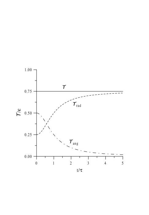
FIG. 1.: Time dependence of the classical-like kinetic energy of a free particle described by the Wigner function (71). $t$ is measured in units of $\tau=M/\alpha^{2}\hbar$, energies in units of $\epsilon=\alpha^{2}\hbar^{2}/M$. The kinetic energy $\cal T$ is separated into its radial part ${\cal T}_{rad}$ and its angular part ${\cal T}_{ang}$.

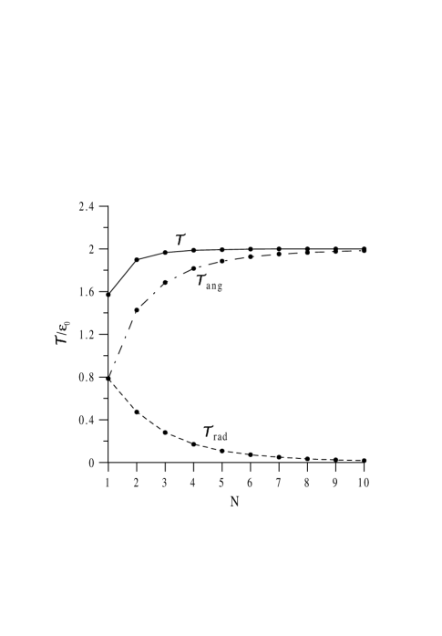
FIG. 2.: With the ground-state wavefunction of the two-dimensional hydrogen atom approximated by a linear combination of $N$ Gaussians, the figure shows the $N$-dependence of the calculated classical-like kinetic energy ${\cal T}$, as well as its radial and angular parts, ${\cal T}_{rad}$ and ${\cal T}_{ang}$. Energies are measured in units of $\epsilon_{0}=\hbar^{2}/Ma_{0}^{2}$.

REFERENCES

• [1] J. P. Dahl, “A Phase Space Essay”, in Conceptual Trends in Quantum Chemistry, edited by E. S. Kryachko and J. L. Calais (Kluwer, The Netherlands, 1994), p. 199.
• [2] J. J. Włodarz, Phys. Letters A 286, 97 (2001).
• [3] J. P. Dahl, in Energy Storage and Redistribution in Molecules, p. 557 (Ed. J. Hinze, Plenum, New York, 1983).
• [4] M. Hug, C. Menke and W. P. Schleich, Phys. Rev. A 57, 3188 and 3206 (1998).
• [5] W. P. Schleich, Quantum Optics in Phase Space (Wiley–VCH, Berlin, 2001).
• [6] J. P. Dahl and M. Springborg, Mol. Phys. 47, 1001 (1982).
• [7] L. Pauling, General Chemistry, 3. ed. (W. H. Freeman & Co., 1970), p. 125.
• [8] We use the word particle in a generalized sense. The $D$ Cartesian coordinates $(x_{1},x_{2},\ldots,x_{D})$ could, for instance, stand for the total set of Cartesian coordinates of $n$ identical particles, instead of the $D$ coordinates of a single individual particle.
• [9] G. Green, Trans. Cambridge Philos. Soc. 5, 395 (1835).
• [10] M. J. M. Hill, Trans. Cambridge Philos. Soc. 13, 273 (1883).
• [11] A. Sommerfeld, Partielle Differentialgleichungen der Physik (Geest & Portig, Leipzig, 1947); Partial Differential Equations in Physics (Academic Press, New York, 1949).
• [12] J. D. Louck, J. Mol. Spectrosc. 4, 298 (1960).
• [13] J. Avery, Hyperspherical Harmonics. Applications in Quantum Theory (Kluwer, London, 1989).
• [14] E. Wigner, Phys. Rev. 40, 749 (1931).
• [15] H. Weyl, The Theory of Groups and Quantum Mechanics (Methuen, London, 1931).
• [16] H. J. Groenewold, Physica 12, 405 (1946).
• [17] J. E. Moyal, Proc. Cambridge Phil. Soc. 45, 99 (1949).
• [18] M. Hillery, R. F. O’Connell, M. O. Scully, and E. P. Wigner, Physics Reports 106, 121 (1984).
• [19] J. P. Dahl, Introduction to the Quantum World of Atoms and Molecules (World Scientific, Singapore, 2001).
• [20] J. P. Dahl, in Dimensional Scaling in Chemical Physics, p. 165 (Eds. D. R. Herschbach, J. Avery and O. Goscinski, Kluwer, Dortrecht, 1993).
Refer to caption