Polarization Squeezing of Continuous Variable Stokes Parameters

Abstract

We report the first direct experimental characterization of continuous variable quantum Stokes parameters. We generate a continuous wave light beam with more than 3 dB of simultaneous squeezing in three of the four Stokes parameters. The polarization squeezed beam is produced by mixing two quadrature squeezed beams on a polarizing beam splitter. Depending on the squeezed quadrature of these two beams the quantum uncertainty volume on the Poincaré sphere became a ‘cigar’ or ‘pancake’-like ellipsoid.

The quantum properties of the polarization of light have received much attention in the single photon regime where fundamental problems of quantum mechanics, related to Bell’s inequality and the Einstein-Podolski-Rosen (EPR) paradox, have been examined AGR82 . In comparison quantum polarization states in the continuous variable regime have received little attention. Grangier et al. GSYL87 generated a polarization squeezed beam using an optical parametric process to improve the sensitivity of a polarization interferometer. Other schemes using Kerr-like media and optical solitons in fibers have also been proposed AAC98 ; KLLRS01 but have not yet been produced experimentally. This paper presents the generation of a new polarization squeezed state. A stably locked beam with better than 3 dB of squeezing in three Stokes parameters simultaneously was produced utilizing two bright quadrature squeezed beams. We present the first direct characterization of the polarization quantum noise on a continuous wave light beam allowing an experimental observation of polarization commutation relations in the continuous variable regime.

Both the production of new continuous variable quantum polarization states and the ability to accurately characterize them are necessary for these states to fulfill their potential in the field of quantum information. They can be carried by a bright laser beam providing high bandwidth capabilities and therefore faster signal transfer rates than single photon systems. Perhaps surprisingly they retain the single photon advantage of not requiring the universal local oscillator necessary for other proposed continuous variable quantum networks. Mapping of quantum states from photonic to atomic media is a crucial element in most proposed quantum information networks. Continuous variable polarization states are the only continuous variable state for which this mapping has been experimentally demonstrated HSSP99 .

The polarization state of a light beam in classical optics can be visualized as a Stokes vector on a Poincaré sphere (Fig. 1) and is determined by the four Stokes parameters Sto52 : $S_{0}$ represents the beam intensity whereas $S_{1}$, $S_{2}$, and $S_{3}$ characterize its polarization and form a cartesian axes system. If the Stokes vector points in the direction of $S_{1}$, $S_{2}$, or $S_{3}$ the polarized part of the beam is horizontally, linearly at 45^∘, or right-circularly polarized, respectively. Two beams are said to be opposite in polarization and do not interfere if their Stokes vectors point in opposite directions. The quantity $\,S=(S_{1}^{2}+S_{2}^{2}+S_{3}^{2})^{1/2}\,$ is the radius of the classical Poincaré sphere and the fraction $\,S/S_{0}\,$ ($\,0\!<\!S/S_{0}\!<\!1\,$) is called the degree of polarization. For quasi-monochromatic laser light which is almost completely polarized $S_{0}$ is a redundant parameter, completely determined by the other three parameters ($S_{0}\!=\!S$ in classical optics). All four Stokes parameters are accessible from the simple experiments shown in Fig. 2.

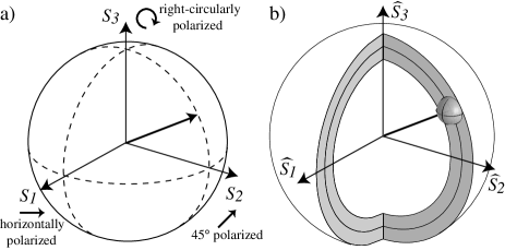
Figure 1: Diagram of a) classical and b) quantum Stokes vectors mapped on a Poincaré sphere; the ball at the end of the quantum vector visualizes the quantum noise in $\rm\hat{S}_{1}$, $\rm\hat{S}_{2}$, and $\rm\hat{S}_{3}$; and the non-zero quantum sphere thickness visualizes the quantum noise in $\rm\hat{S}_{0}$.

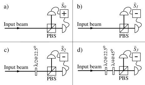
Figure 2: Apparatus required to measure each of the Stokes parameters. PBS: polarizing beam splitter, $\lambda/2$ and $\lambda/4$: half- and quarter-wave plates respectively, the plus and minus signs imply that an electrical sum or difference has been taken.

The Stokes parameters are observables and therefore can be associated with Hermitian operators. Following JauchRohrlich76 and Robson74 we define the quantum-mechanical analogue of the classical Stokes parameters for pure states in the commonly used notation:

$$\hat{S}_{0} \!=\hat{a}_{H}^{\dagger}\hat{a}_{H}+\hat{a}_{V}^{\dagger}\hat{a}_{V}~{},\hskip 5.69054pt\hat{S}_{2} \!=\hat{a}_{H}^{\dagger}\hat{a}_{V}e^{i\theta}\!+\hat{a}_{V}^{\dagger}\hat{a}_{H}e^{-i\theta},\;\;\;\;\;\;$$ (1)

$$\hat{S}_{1} \!=\hat{a}_{H}^{\dagger}\hat{a}_{H}-\hat{a}_{V}^{\dagger}\hat{a}_{V}~{},\hskip 5.69054pt\hat{S}_{3} \!=i\hat{a}_{V}^{\dagger}\hat{a}_{H}e^{-i\theta}\!-i\hat{a}_{H}^{\dagger}\hat{a}_{V}e^{i\theta},\;\;\;\;\;\;$$

where the subscripts $H$ and $V$ label the horizontal and vertical polarization modes respectively, $\theta$ is the phase shift between these modes, and the $\hat{a}_{H,V}$ and $\hat{a}_{H,V}^{\dagger}$ are annihilation and creation operators for the electro-magnetic field in frequency space. The commutation relations of these operators

$$[\hat{a}_{k},\hat{a}_{l}]=\delta_{kl}~{},\hskip 11.38109pt\mbox{with}\hskip 11.38109ptk,l\in\{H,V\}~{},$$ (2)

directly result in Stokes operator commutation relations,

$$[\hat{S}_{1},\hat{S}_{2}]=2i\hat{S}_{3}~{},\hskip 5.69054pt[\hat{S}_{2},\hat{S}_{3}]=2i\hat{S}_{1}~{},\hskip 5.69054pt[\hat{S}_{3},\hat{S}_{1}]=2i\hat{S}_{2}~{}\,.$$ (3)

Apart from a normalization factor, these relations are identical to the commutation relations of the Pauli spin matrices. In fact the three Stokes parameters in Eq. (3) and the three Pauli spin matrices both generate the special unitary group of symmetry transformations SU(2) of Lie algebra Kaku93 . Since this group obeys the same algebra as the three-dimensional rotation group, distances in three dimensions are invariant. Accordingly the operator $\hat{S}_{0}$ is also invariant and commutes with the other three Stokes operators ($\,[\hat{S}_{0},\hat{S}_{j}]=0,\;\mbox{with}\;j=1,2,3$). It can be shown from Eqs. (1) and (2) that the quantum Poincaré sphere radius is different from its classical analogue, $\,\langle\hat{S}\rangle=\langle\hat{S}_{0}^{2}+2\hat{S}_{0}\rangle^{1/2}\,$. The noncommutability of the Stokes operators $\hat{S}_{1}$, $\hat{S}_{2}$ and $\hat{S}_{3}$ precludes the simultaneous exact measurement of their physical quantities. Their mean values $\,\langle\hat{S}_{j}\rangle\,$ and variances $\,V_{j}=\langle\hat{S}_{j}^{2}\rangle\!-\!\langle\hat{S}_{j}\rangle^{2}\,$ are restricted by the uncertainty relations JauchRohrlich76

$$V_{1}V_{2}\geq|\langle\hat{S}_{3}\rangle|^{2}~{},~{}V_{2}V_{3}\geq|\langle\hat{S}_{1}\rangle|^{2}~{},~{}V_{3}V_{1}\geq|\langle\hat{S}_{2}\rangle|^{2}~{}.$$ (4)

In general this results in non-zero variances in the individual Stokes parameters as well as in the radius of the Poincaré sphere (see Fig. 1b)). Recently it has been shown that these variances may be obtained from the frequency spectrum of the electrical output currents of the setups shown in Fig. 2 KLLRS01 .

It is useful to express the Stokes operators of Eq. (1) in terms of quadrature amplitudes of the horizontally and vertically polarized components of the beam. The creation and annihilation operators can be expressed as sums of real classical amplitudes $\alpha_{H,V}$ and quadrature quantum noise operators $\delta\hat{X}_{H,V}^{+}$ and $\delta\hat{X}_{H,V}^{-}$ WallsMilburn

$$\hat{a}_{H,V}=\alpha_{H,V}+\frac{1}{2}(\delta\hat{X}_{H,V}^{+}+i\delta\hat{X}_{H,V}^{-})~{}.$$ (5)

If the variances of the noise operators are much smaller than the coherent amplitudes then, to first order in the noise operators, the Stokes operator mean values are

$$\langle\hat{S}_{0}\rangle = \alpha_{H}^{2}+\alpha_{V}^{2}=\langle\hat{n}\rangle~{},\hskip 5.69054pt\langle\hat{S}_{2}\rangle=2\alpha_{H}\alpha_{V}\,\mbox{cos}\theta~{},$$ (6)

$$\langle\hat{S}_{1}\rangle = \alpha_{H}^{2}-\alpha_{V}^{2}~{},\hskip 32.72066pt\langle\hat{S}_{3}\rangle=2\alpha_{H}\alpha_{V}\,\mbox{sin}\theta~{},$$

where $\,\langle\hat{n}\rangle\,$ is the expectation value of the photon number operator. For a coherent beam the expectation value and variance of $\hat{n}$ have the same magnitude, this magnitude equals the conventional shot-noise level. The variances of the Stokes parameters are given by

$$V_{0}=V_{1}= \!\alpha_{H}^{2}\langle(\delta\hat{X}_{H}^{+})^{2}\rangle\!+\!\alpha_{V}^{2}\langle(\delta\hat{X}_{V}^{+})^{2}\rangle,\;\;\;\;$$

$$V_{2}(\theta\!=\!0)\!=\!V_{3}(\theta\!=\!\pi\!/2)= \!\alpha_{V}^{2}\langle(\delta\hat{X}_{H}^{+})^{2}\rangle\!+\!\alpha_{H}^{2}\langle(\delta\hat{X}_{V}^{+})^{2}\rangle,\;\;\;\;$$ (7)

$$V_{3}(\theta\!=\!0)\!=\!V_{2}(\theta\!=\!\pi\!/2)= \!\alpha_{V}^{2}\langle(\delta\hat{X}_{H}^{-})^{2}\rangle\!+\!\alpha_{H}^{2}\langle(\delta\hat{X}_{V}^{-})^{2}\rangle,\;\;\;\;$$

The variances of the noise operators in the above equation are normalized to one for a coherent beam. Therefore the variances of the Stokes parameters of a coherent beam are all equal to the shot-noise of the beam. For this reason a Stokes parameter is said to be squeezed if its variance falls below the shot-noise of an equal power coherent beam. Although the decomposition to the $H,V$-polarization axis of Eqs. (Polarization Squeezing of Continuous Variable Stokes Parameters) is independent of the actual procedure of generating a polarization squeezed beam, it becomes clear that two overlapped quadrature squeezed beams can produce a single polarization squeezed beam. We choose the two specific angles of $\,\theta\!=\!0$ and $\pi/2\,$ in Eqs. (Polarization Squeezing of Continuous Variable Stokes Parameters) corresponding to our actual experimental setup. If the polarization squeezed beam is generated from two amplitude squeezed beams $\hat{S}_{0}$ and two additional Stokes parameters can in theory be perfectly squeezed while the fourth is anti-squeezed. In this case the uncertainty volume formed by the noise variances of the Stokes parameters in the Poincaré space becomes a “cigar”-like ellipsoid. If the polarization squeezed beam is generated from two phase squeezed beams the uncertainty volume becomes a “pancake”-like ellipsoid (see Fig. 5).

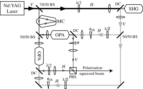
Figure 3: Schematic of the polarization squeezing experiment. BS: beam splitter, DC: dichroic beam splitter, $\lambda/2$: half-wave plate, $\phi_{sh}$: phase shift between 532 nm and 1064 nm light at the OPAs, $\theta$: phase shift between quadrature squeezed beams, PBS: polarizing beam splitter.

The experimental setup used to generate the polarization squeezed beams is shown in Fig. 3. Two quadrature squeezed beams were produced in a pair of spatially separated optical parametric amplifiers (OPAs). Past experiments requiring two quadrature squeezed beams commonly used a single ring resonator with two outputs Ou ; with two independent OPAs the necessary intracavity pump power is halved, this reduces the degradation of squeezing due to green-induced infrared absorption (GRIIRA) Furukawa . The OPAs were optical resonators constructed from hemilithic MgO:LiNbO₃ crystals and output couplers. The reflectivities of the output couplers were 96% and 6% for the fundamental (1064 nm) and the second harmonic (532 nm) laser modes, respectively. The OPAs were pumped with single-mode 532 nm light generated by a 1.5 W Nd:YAG non-planar ring laser and frequency doubled in a second harmonic generator (SHG). The SHG was of identical structure to the OPAs but with 92% reflectivity at 1064 nm. Each OPA was seeded with 1064 nm light after spectral filtering in a modecleaner. This seed enabled control of the length of the OPAs. The coherent amplitude of each OPAs output was a deamplified/amplified version of the seed coherent amplitude; the level of amplification was dependent on the phase difference between pump and seed ($\phi_{sh}$). Locking to deamplification or amplification provided amplitude or phase squeezed outputs, respectively.

The two quadrature squeezed beams were combined with orthogonal polarization on a polarizing beam splitter, similarly to a scheme proposed for solitons KLLRS01 . This produced an output beam with Stokes parameter variances as given by Eqs. (Polarization Squeezing of Continuous Variable Stokes Parameters). Both input beams had equal power ($\alpha_{H}\!=\!\alpha_{V}\!=\!\alpha/\sqrt{2}$) and both were squeezed in the same quadrature. The Stokes parameters and their variances were determined as shown in Fig. 2. The beam was split on a polarizing beam splitter and the two outputs were detected on a pair of high quantum efficiency photodiodes with 30 MHz bandwidth; the resulting photocurrents were added and subtracted to yield the means and variances of $\hat{S}_{0}$ and $\hat{S}_{1}$. To measure $\langle\hat{S}_{2}\rangle$ and $V_{2}$ the polarization of the beam was rotated by 45^∘ with a half-wave plate before the polarizing beam splitter and the detected photocurrents were subtracted. To measure $\langle\hat{S}_{3}\rangle$ and $V_{3}$ the polarization of the beam was rotated by 45^∘ with a half-wave plate and a quarter-wave plate was introduced before the polarizing beam splitter such that a horizontally polarized input beam became right-circular. Again the detected photocurrents were subtracted. The relative phase between the quadrature squeezed input beams $\theta$ was locked to $\pi/2$ rads producing in all cases a right-circularly polarized beam with Stokes parameter means of $\langle\hat{S}_{1}\rangle\!=\!\langle\hat{S}_{2}\rangle\!=\!0$ and $\langle\hat{S}_{0}\rangle\!=\!\langle\hat{S}_{3}\rangle\!=\!|\alpha|^{2}$. There is no fundamental bias in the orientation of the quantum Stokes vector. By varying the angle of an additional half-wave plate in the polarization squeezed beam and by varying $\theta$ any orientation may be achieved. In fact the experiment discussed here was also carried out with $\theta$ locked to 0 rads, in this case the Stokes vector was rotated to point along $\hat{S}_{2}$ and the quantum noise was similarly rotated. Near identical results were obtained but on alternative Stokes parameters.

Each quadrature squeezed beam had an overall detection efficiency of 73%. The loss came primarily from four sources: loss in escape from the OPAs (14%), detector inefficiency (7%), loss in optics (5%), and mode overlap mismatch between the beams (4%). Depolarizing effects are thought to be another significant source of loss for some polarization squeezing proposals APu89 . In our scheme the non-linear processes (OPAs) are divorced from the polarization manipulation (wave plates and polarizing beam splitters), and depolarizing effects are insignificant.

As discussed earlier the Stokes parameters of a beam are squeezed if their variances fall below the shot-noise level of an equally intense coherent beam. This shot-noise level was used to calibrate the measurements presented here, it was determined by operating a single OPA without the second harmonic pump. The seed power was adjusted so that the output power was equal to that of the polarization squeezed beam. In this configuration the detection setup for $\hat{S}_{2}$ (see Fig. 2c)) functions exactly as a homodyne detector measuring vacuum noise scaled by the OPA output power the variance of which is the shot-noise. Throughout each experimental run the sum of output powers from the two OPAs was monitored and was always within 2% of the power of the coherent calibration beam. This led to a conservative error in our frequency spectra of $\pm$0.04 dB.

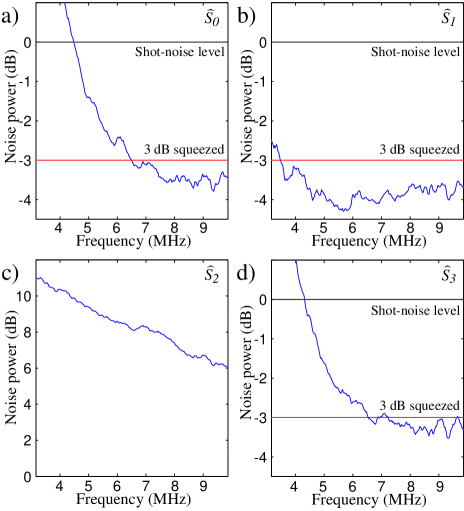
Figure 4: Measured variance spectra of quantum noise on a) $\hat{S}_{0}$, b) $\hat{S}_{1}$, c) $\hat{S}_{2}$, and d) $\hat{S}_{3}$ for locked amplitude squeezed input beams; normalized to shot-noise.

The shot-noise and Stokes parameter variances presented here were taken with a Hewlett-Packard E4405B spectrum analyzer over the range from 3 to 10 MHz. The darknoise of the detection apparatus was always more than 4 dB below the measured traces and was taken into account. Each displayed trace is the average of three measurement results normalized to the shot-noise and smoothed over the resolution bandwidth of the spectrum analyzer which was set to 300 kHz. The video bandwidth of the spectrum analyzer was set to 300 Hz.

Fig. 4 shows the measurement results obtained with both input beams amplitude squeezed. $\hat{S}_{0}$, $\hat{S}_{1}$ and $\hat{S}_{3}$ are all squeezed from 4.5 MHz to the limit of our measurement, 10 MHz. $\hat{S}_{2}$ is anti-squeezed throughout the range of the measurement. Between 7.2 MHz and 9.6 MHz $\hat{S}_{0}$, $\hat{S}_{1}$ and $\hat{S}_{3}$ are all more than 3 dB below shot-noise. The squeezing of $\hat{S}_{0}$ and $\hat{S}_{3}$ is degraded at low frequency due to phase noise on the second harmonic pump coupling into the amplitude quadrature of the OPA outputs. Since this noise is correlated it cancels in the variance of $\hat{S}_{1}$. The maximum squeezing of $\hat{S}_{0}$ and $\hat{S}_{2}$ was 3.8 dB and 3.5 dB respectively and was observed at 9.3 MHz. The maximum squeezing of $\hat{S}_{1}$ was 4.3 dB at 5.7 MHz. The repetitive structure at 4, 5, 6, 7, 8 and 9 MHz was caused by electrical pick-up in our SHG resonator emitted from a separate experiment operating in the laboratory.

By locking both OPAs to amplification we obtained results similar to those in Fig. 4 but with the input beams phase squeezed. In this case $\hat{S}_{0}$, $\hat{S}_{1}$ and $\hat{S}_{3}$ were all anti-squeezed and $\hat{S}_{2}$ was squeezed throughout the range of the measurement. The optimum noise reduction of $\hat{S}_{2}$ was 2.8 dB below shot-noise and was observed at 4.8 MHz.

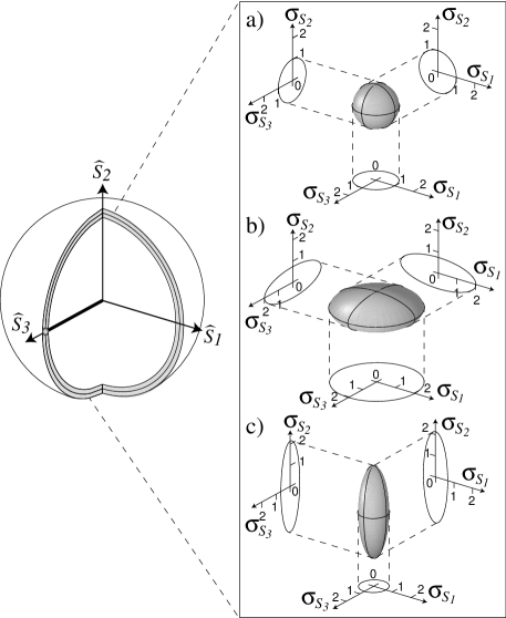
Figure 5: Measured quantum polarization noise at 8.5 MHz mapped onto the Poincaré sphere. a) coherent beam, b) beam from two phase squeezed inputs, c) beam from two amplitude squeezed inputs. The surface of the ellipsoids defines the standard deviation of the noise normalized to shot-noise ($\sigma_{S_{i}}\!=\!\sqrt{V_{i}}$).

In Fig. 5 we visualize our experimental data at 8.5 MHz assuming Gaussian noise statistics. Given this assumption, the standard deviation contour-surfaces shown here provide an accurate representation of the states three dimensional noise distribution. The quantum polarization noise of a coherent state forms a sphere of noise as portrayed in Fig. 5 a). The noise volume formed by our experimental results with two phase or two amplitude squeezed beams respectively, was found to be a ‘pancake’-like (Fig. 5 b)) or ‘cigar’-like ellipsoid (Fig. 5 c)).

In all experiments prior to this work involving polarization squeezing the squeezing was generated by combining a strong coherent beam with a single weak amplitude squeezed beam GSYL87 ; HSSP99 . Utilizing only one squeezed beam it is not possible to simultaneously squeeze any two of $\hat{S}_{1}$, $\hat{S}_{2}$, and $\hat{S}_{3}$ to quieter than 3 dB below shot-noise ($V_{i}\!+\!V_{j}\!\geq\!\langle\hat{n}\rangle$, with $i,j\in\{1,2,3;i\!\not=\!j\}$). This can be seen from the more general form of Eqs. (Polarization Squeezing of Continuous Variable Stokes Parameters) which includes arbitrary phase angle $\theta$ between the beams.

To conclude, we present the first direct experimental characterization of continuous variable quantum Stokes parameters. We generate a new quantum state with better than 3 dB squeezing of three Stokes parameters ($\hat{S}_{0}$, $\hat{S}_{1}$, and $\hat{S}_{3}$) simultaneously, a quality impossible to produce with only one squeezed beam. We represent our results on a quantum version of the Poincaré sphere and experimentally demonstrate that in this space a polarization squeezed beam generated from two amplitude squeezed beams has a ‘cigar’-like quantum noise distribution; and one from two phase squeezed beams has a ‘pancake’-like quantum noise distribution.

We would like to acknowledge the Alexander von Humboldt foundation for support of Dr. R. Schnabel; the Australian Research Council for financial support; Dr. M. B. Gray and Dr. B. C. Buchler for technical assistance; and Dr. T. C. Ralph for useful discussion.

References

- (1) A. Aspect, P. Grangier, and G. Roger, Phys. Rev. Lett. 49, 91 (1982).
- (2) P. Grangier, R. E. Slusher, B. Yurke, and A. LaPorta, Phys. Rev. Lett. 59, 2153 (1987).
- (3) A. P. Alodjants, S. M. Arakelian, and A. S. Chirkin, Appl. Phys. B 66, 53 (1998).
- (4) N. V. Korolkova, G. Leuchs, R. Loudon, T. C. Ralph, and C. Silberhorn, quant-ph/0108098.
- (5) J. Hald, J. L. Sørensen, C. Schori, and E. S. Polzik, Phys. Rev. Lett. 83 1319 (1999).
- (6) G. G. Stokes, Trans. Camb. Phil. Soc. 9, 399 (1852).
- (7) J. M. Jauch and F. Rohrlich, The Theory of Photons and Electrons, 2nd ed., (Springer, Berlin, 1976).
- (8) B. A. Robson, The Theory of Polarization Phenomena, (Clarendon, Oxford, 1974).
- (9) See for example M. Kaku, Quantum Field Theory, (Oxford University Press, New York, 1993).
- (10) D. F. Walls and G. J. Milburn, Quantum Optics, (Springer, Berlin, 1995).
- (11) See for example Z. Y. Ou, S. F. Pereira, H. J. Kimble, and K. C. Peng, Phys. Rev. Lett. 68, 3663 (1992).
- (12) Y. Furukawa, K. Kitamura, A. Alexandrovski, R. K. Route, M. M. Fejer, and G. Foulon, Appl. Phys. Lett. 78, 1970 (2001).
- (13) G. S. Agarwal and R. .R. Puri, Phys. Rev. A40, 5179 (1989).