AC-driven quantum spins: resonant enhancement of transverse DC magnetization

Abstract

We consider $s=1/2$ spins in the presence of a constant magnetic field in $z$-direction and an AC magnetic field in the $x-z$ plane. A nonzero DC magnetization component in $y$ direction is a result of broken symmetries. A pairwise interaction between two spins is shown to resonantly increase the induced magnetization by one order of magnitude. We discuss the mechanism of this enhancement, which is due to additional avoided crossings in the level structure of the system.

I Introduction

Magnetic resonance effects have been long studied and used for various spectroscopic methods [1, 2, 3]. Time-dependent external fields being an integral part of the physical setups, become also very interesting in their action when entering the field of spintronics and processing of quantum information [4]. While the linear response of a system (probe) to external fields may be typically understood in a rather complete way, nonlinear and perhaps nonadiabatic response effects are usually much harder to be analyzed. Some studies have been devoted to the effect of second-harmonic generation. Much less is known about zeroth-harmonic generation, i.e. about the induction of static fields by pure ac fields. The understanding of such processes is very important in any application involving ac fields, as additional induced dc fields may strongly influence the desired effects.

The principal possibility of the zeroth-harmonic generation can be studied using symmetry considerations [5],[6]. Analytical approaches which may also estimate the magnitude of the induced fields are typically restricted to various perturbation techniques with a suitable small parameter involved. Two of us have recently applied these methods to the simplest cases of a spin $s=1/2$ coupled to an environment (heat bath) in the presence of an external magnetic dc field (in $z$-direction) [7]. While an additional ac field applied in $x$-direction leads to the standard spin resonance setup used e.g. for nuclear spins, a tilt of the ac field direction in the $x-z$-plane leads to a broken symmetry and to a generation of a nonzero magnetic moment in $y$-direction, i.e. perpendicular to the applied fields. Similar results have been also obtained for a spin $s=1$ where the external dc field in $z$-direction is replaced by a magnetic ion anisotropy in $z$-direction [7].

This work is devoted to the analysis of spin-spin interaction and its action on the above described effects. The first goal is to study the generalization of the symmetry considerations in the presence of an interaction. The second goal is to demonstrate that the interaction is capable of increasing the induced field strength by an order of magnitude, and to give an explanation for this result.

The paper is organized as follows. In the next section we introduce the density matrix approach. Section III is devoted to a reconsideration of the single spin problem. Section IV contains the central results on two interacting spins. Section V concludes the paper.

II The density matrix approach

In this section we introduce the methods we are using. Let us assume that a single spin or a system of interacting spins is represented by a time-dependent Hamiltonian $H(t)=H_{0}+H_{1}(t)$ which includes both applied dc and ac magnetic fields. Here the static part is completely included in $H_{0}$ and the action of the ac fields is described by a time-periodic term $H_{1}(t)=H_{1}(t+T)$ with period $T$. In order to describe the time-dependent statistical evolution of such a system we use the quantum Liouville equation for the density matrix $\rho(t)$

$$\frac{\partial\rho}{\partial t}=i[H,\rho]-\nu(\rho-\rho_{e})$$ (1)

where $[A,B]=AB-BA$. While the specifics of the internal dynamics of the system are described by the first term on the rhs of (1), the second term accounts for the interaction of our spin system with an environment. We will handle this interaction in a rather qualitative way. The principal request this coupling should fulfill is that its action should preserve all symmetries of $H(t)$ except time reversal symmetry. A second requirement is that the solution of (1) in the absence of ac fields $H_{1}(t)=0$ should be the Gibbs distribution

$$\rho_{\beta}(H_{0})=\frac{1}{Z_{0}}e^{-\beta H_{0}}\;,\;Z_{0}=Tr(e^{-\beta H_{0}})\;\;.$$ (2)

Finally we request that all solutions of (1) should approach a unique time-dependent state.

The choice $\rho_{e}=\rho_{\beta}(H_{0})$ satisfies the above criteria. As shown in [7] for $s=1/2$ it leads to equations practically identical with the well known Bloch equations. However e.g. for adiabatically slow ac fields a much better choice would be $\rho_{e}\equiv\rho_{\beta}(H(t))=\frac{1}{Z}e^{-\beta H(t)}$. We will discuss the subtle differences below. In general however we may state here that any of the two choices fulfills the above criteria. Note that the third criterium (unique asymptotic behaviour) is guaranteed, as a linear equation like (1) exhibits one and only one attractor, and the whole phase space serves as a region of attraction for this single attractor. Note that due to $Tr\rho_{\beta}=1$ any choice with $Tr\rho(0)=1$ implies $Tr\rho(t)=1$ for all $t$.

The value $\bar{A}(t)$ of an observable corresponding to the operator $A$ is defined by

$$\bar{A}(t)=Tr(A\rho(t))$$ (3)

and its time average is abbrevated by

$$\tilde{A}=\frac{1}{T}\int_{0}^{T}\bar{A}(t)\,dt.$$ (4)

III Revisiting a single spin $s=\frac{1}{2}$

We consider one spin $s=1/2$ in the presence of a constant magnetic field in $z$-direction and a time-periodic magnetic field with angle $\phi$ to the $z$-axis in $z-x$-plane. The Hamiltonian is given by

$$H(t)=h_{0}S_{z}+h(t)(\alpha S_{x}+\gamma S_{z}),$$ (5)

where $\alpha=\sin\phi$ and $\gamma=\cos\phi$. We assume that the field $h(t)=h(t+T)$ has zero mean $\int_{0}^{T}h(t)\,dt=0$.

The spin component operators are given by the Pauli matrices: $S_{x,y,z}=\frac{1}{2}\sigma_{x,y,z}$. The density matrix $\rho=R+iI$ can be decomposed into a real symmetric $2\times 2$ matrix $R$ and a real antisymmetric $2\times 2$ matrix $I$ and has three independent variables. Using the relation (3), we rewrite the system (1) in terms of $\bar{S}_{x,y,z}$

$$\dot{\bar{S}}_{x} = (h_{0}+\gamma h(t))\bar{S}_{y}-\nu\bar{S}_{x}$$ (6)

$$\dot{\bar{S}}_{y} = \alpha h(t)\bar{S}_{z}-(h_{0}+\gamma h(t))\bar{S}_{x}-\nu\bar{S}_{y}$$ (7)

$$\dot{\bar{S}}_{z} = -\alpha h(t)\bar{S}_{y}-\nu(\bar{S}_{z}+C)$$ (8)

where $C=\frac{1}{2}\tanh(\beta h_{0}/2)$. The structure of these equations is equivalent to the wellknown Bloch equations provided the relaxation times there would be chosen to be identical [2]. Note that the symmetries of the equations (6) are identical with the ones of the corresponding Bloch equations.

Because of the presence of a time-periodic field, for times $t\gg 1/\nu$ all components $\bar{S}_{x,y,z}$ will be also time periodic with period $T$ or frequency $\omega=2\pi/T$. We can expand the solution of system (6) in a Fourier series

$$\bar{S}_{x,y,z}=A_{0\;x,y,z}+\sum\limits_{n\not=0}e^{i\omega nt}A_{n\;x,y,z}\;\;.$$ (9)

After averaging over the period $T$, we have

$$\tilde{S}_{x,y,z}=A_{0\;x,y,z}\;\;.$$ (10)

The symmetry analysis of the equations (6) yields the following results [7] (we considered only operations which conserve $Tr\rho$):
1) $\nu=0$, $\gamma=0\;,\;h(-t)=-h(t)$:

$$\bar{S}_{x}\rightarrow-\bar{S}_{x}\;,\;\bar{S}_{y}\rightarrow\bar{S}_{y}\;,\;\bar{S}_{z}\rightarrow\bar{S}_{z}\;,\;t\rightarrow-t.$$ (11)

2) $\nu=0$, for all $\gamma\;,\;h(-t)=h(t)$:

$$\bar{S}_{x}\rightarrow\bar{S}_{x}\;,\;\bar{S}_{y}\rightarrow-\bar{S}_{y}\;,\;\bar{S}_{z}\rightarrow\bar{S}_{z}\;,\;t\rightarrow-t.$$ (12)

3) $\nu\not=0$, $\gamma=0,\;\;h(t+T/2)=-h(t)$:

$$\bar{S}_{x}\rightarrow-\bar{S}_{x}\;,\;\bar{S}_{y}\rightarrow-\bar{S}_{y}\;,\;\bar{S}_{z}\rightarrow\bar{S}_{z}\;,\;t\rightarrow t+\frac{T}{2}\;.$$ (13)

If any of the above symmetries hold in a relevant parameter case, the corresponding components of $\tilde{S}$ will exactly vanish. E.g. for case 1) $\tilde{S}_{x}=0$, for case 2) $\tilde{S}_{y}=0$ and for case 3) $\tilde{S}_{x}=\tilde{S}_{y}=0$. The key idea now is that a proper choice of the parameters (including the time dependence of $h(t)$) may lead to a violation of all symmetries. As a consequence we expect nonzero values of the corresponding $A_{0\;x,y}$. This means that even if we do not apply an external magnetic field in $y$-direction, we can expect a nonzero $\tilde{S}_{y}$ component, which will be a function of the ac field frequency $\omega$. In order to quantify the zeroth harmonic generation we use the following definition of the strength of the effect $I_{NL}$:

$$I_{NL}=\frac{\max\limits_{\omega}|\tilde{S}_{y}|}{\max\limits_{\omega}|\tilde{S}_{z}|}\cdot 100\%$$ (14)

Let us emphasize here that the denominator in (14) is of nonresonant character, i.e. its value is determined by the maximum values of $\tilde{S}_{z}$ which is obtained for frequency values far from the magnetic resonance and practically coincides with the equilibrium value for zero ac fields. In contrast the enumerator gets its maximum (if nonzero et al) inside some resonance window in $\omega$.

In [7] a perturbation theory was developed for strong dissipation $1/\nu\ll 1$. Here we will account for the effect assuming a small amplitude of the ac field $h(t)=\epsilon\cos(\omega t)$, $\epsilon\ll 1$ and $\epsilon<\nu$:

$$A_{0\;x} = -\epsilon^{2}\frac{\alpha\gamma C(\nu^{2}+\omega^{2}-h_{0}^{2})}{2\Delta}+o(\epsilon^{3})$$ (15)

$$A_{0\;y} = \epsilon^{2}\frac{\alpha\gamma\nu h_{0}C}{\Delta}+o(\epsilon^{3})$$ (16)

$$A_{0\;z} = -C+\epsilon^{2}\frac{\alpha^{2}C(\nu^{2}+\omega^{2}+h_{0}^{2})}{2\Delta}+o(\epsilon^{3})$$ (17)

where $\Delta=(h_{0}^{2}-\omega^{2})^{2}+\nu^{2}(\nu^{2}+2h_{0}^{2}+2\omega^{2})$. The dependence of $A_{0\;x,y,z}$ on $\omega$ shows the expected resonant character. A nonzero component of $\tilde{S}_{y}$, being a nonlinear response result, appears in second order of the ac field amplitude $\epsilon$.

For the case of the magnetic resonance $\omega=h_{0}$ we find

$$A_{0\;x} \approx -\epsilon^{2}\frac{\alpha\gamma C}{2h_{0}^{2}(4+\xi^{2})}$$ (18)

$$A_{0\;y} \approx \epsilon^{2}\frac{\alpha\gamma C}{\xi h_{0}^{2}(4+\xi^{2})}\$$ (19)

where $\xi=\frac{\nu}{h_{0}}$.

To test the possible magnitude of the effect, we compute the induced moments numerically following [7]. The results are the solid lines in Fig.1. While the resonance character is clearly observable, the strength $I_{NL}\approx 3.0\%$ is rather small.

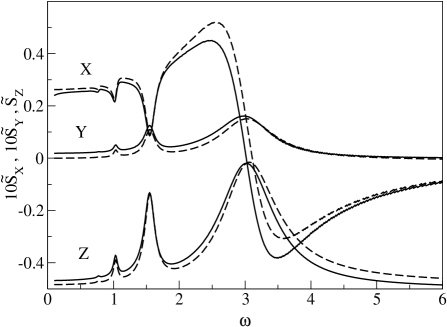
FIG. 1.: $\tilde{S}_{x,y,z}$ as function of $\omega$. Chosen parameters are: $h_{0}=3.0$, $\phi=\frac{\pi}{4}$, $\beta=10$, $\nu=0.1$, $h(t)=\sqrt{2}\cos(\omega t)$. Solid lines: $\rho_{e}=\rho_{\beta}(H_{0})$. Dashed lines: $\rho_{e}=\rho_{\beta}(H(t))$

In addition, one can see that in the adiabatic limit $\omega\rightarrow 0$ $\tilde{S}_{y}$ keeps a small but nonzero value. This is in contrast to the expectation that for very slowly varying ac fields the spin system should momentarily adjust to the actual field value, which implies a zero average $y$-component of the induced moment. As already discussed above, a much better choice in this limit would be $\rho_{e}=\rho_{\beta}(H(t))$. A computation with this choice is shown also in Fig.1 (dashed lines). We find that while the overall difference in the results for the two choices for $\rho_{e}$ are small, the adiabatic limit is correctly reproduced by the second one as expected.

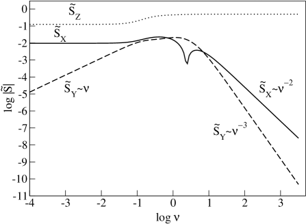
FIG. 2.: $\log\tilde{S}_{x,y,z}$ as function of $\log\nu$ for $\omega=1.5$, other parameters as in Fig.1. $\tilde{S}_{x}$: solid line, $\tilde{S}_{y}$ - dashed line, $\tilde{S}_{z}$ - dotted line.

It is also instructive to study the dependence of the values of $\tilde{S}_{x,y,z}$ as a function of the dissipation $\nu$. In Fig.2 we plot this dependence for the subresonance case $\omega=1.5$ from Fig.1. We observe that $\tilde{S}_{z}$ shows a kink around $\nu=0.1$. The $\tilde{S}_{x}$ curve provides with the a $\sim 1/\nu^{2}$ decay for large $\nu$, as expected from perturbation theory. Except for a small dip around $\nu=2$ it then saturates at a nonzero value for small $\nu$ values. This is in full agreement with the above symmetry statements. Finally the $\tilde{S}_{y}$ curve shows a $\sim 1/\nu^{3}$ decay for large $\nu$, again as expected from perturbation theory. Notably $\tilde{S}_{y}$ tends to zero also for small dissipation values, in full accord with the above symmetry statements.

IV Two interacting spins

In order to enhance the value of $I_{NL}$ we may either consider larger spins or effects of interactions between spins. In [7] the case of $s=1$ has been considered, with the result that $I_{NL}$ is not significantly changed as compared to $s=1/2$. Consequently we turn in this section to the consideration of spin interactions. In the following we will study a system of two interacting spins $s=1/2$, which could be realized through the interactions e.g. in a molecule. As we are interested in the qualitative effects such an interaction might induce, we choose the mathematically simple version of exchange interaction. We think that e.g. dipole-dipole interactions as realized between nuclear spins will not significantly alter the picture.

Our starting Hamiltonian is given by

$$H = h_{0}(S_{z}^{1}+S_{z}^{2})+h(t)(\alpha(S_{x}^{1}+S_{x}^{2})+\gamma(S_{z}^{1}+S_{z}^{2}))-$$ (20)

$$- J_{x}S_{x}^{1}S_{x}^{2}-J_{y}S_{y}^{1}S_{y}^{2}-J_{z}S_{z}^{1}S_{z}^{2}$$ (21)

with $h(t+T)=h(t)$, $\alpha=\sin(\phi)$ and $\gamma=\cos(\phi)$. For two spins $s=1/2$ the above operators $S_{x,z}^{1,2}$ take the form $S_{x,z}^{1}=\frac{1}{2}\sigma_{x,z}\bigotimes\mathbf{1}$, $S_{x,z}^{2}=\mathbf{1}\mathnormal{\bigotimes}\frac{1}{2}\sigma_{x,z}$ where $\sigma_{x,z}$ are Pauli matrices, $\mathbf{1}$ denotes the $2\times 2$ unity matrix and $\bigotimes$ stands for the tensorial product of operators (matrices).

In this case the matrix $\rho=R+iI$ contains 15 independent variables.

We define the total components of spins as $S_{x,y,z}=\frac{1}{2}(S_{x,y,z}^{1}+S_{x,y,z}^{2})$. With the help of (3) it follows

$$\bar{S}_{x} = \frac{1}{2}(R_{12}+R_{13}+R_{24}+R_{34})$$ (22)

$$\bar{S}_{y} = \frac{1}{2}(I_{12}+I_{13}+I_{24}+I_{34})$$ (23)

$$\bar{S}_{z} = \frac{1}{2}(R_{11}-R_{44})$$ (24)

The symmetry analysis of this system is identical to the case of one spin $s=1/2$ (13-12). The existence of additional parameters (exchange coefficients) does not reduce the symmetries nor add some. The only important additional point is that changes of signs of the expectation values of a given spin component operator have to be done simultaneously for both spins once the interaction is nonzero.

A Isotropic exchange

Let us first consider the case of isotropic exchange $J_{x}=J_{y}=J_{z}\equiv J$.

First we note that with the help of a unitary transformation we can transform the Hamiltonian (20) into a triplet-singlet representation. The singlet state (total spin $s=0$) decouples from the three triplet states (total spin $s=1$). The time-dependent part of (20) is contained in the triplet part. For a given value of the ac field the eigenvalues of the singlet state $E_{0}$ and the three triplet states $E_{1,2,3}$ are given by

$$E_{0} = \frac{3}{4}J$$ (25)

$$E_{1} = -\frac{1}{4}J+\sqrt{a^{2}+4c^{2}},$$ (26)

$$E_{2} = -\frac{1}{4}J,$$ (27)

$$E_{3} = -\frac{1}{4}J-\sqrt{a^{2}+4c^{2}}$$ (28)

where $a=h_{0}+\gamma\cos(\omega t)$ and $c=\frac{1}{2}\alpha\cos(\omega t)$.

On one side the singlet state is not interacting with the triplet states and all spin component expectation values in this singlet state are exactly zero. On the other side the singlet state is consuming statistical weight. Thus the dynamics of the system of two spins one-half interacting via isotropic exchange and coupled to a heat bath can be reduced to the dynamics of a single spin $s=1$ (triplet states) with a reduced statistical weight. For the case of $\rho_{e}=\rho_{\beta}(H_{0})$ this reduced statistical weight is given by

$$C_{1}=\frac{Tr(e^{-\beta H_{0}^{\prime}})}{Tr(e^{-\beta H_{0}})}$$ (29)

where $H_{0}^{\prime}$ is obtained from $H_{0}$ by excluding the singlet state. Using $Tr(e^{-\beta H_{0}^{\prime}})=2e^{\frac{\beta J}{4}}\cosh(\beta h_{0})+e^{\frac{\beta J}{4}}$ and $Tr(e^{-\beta H_{0}})=Tr(e^{-\beta H_{0}^{\prime}})+e^{-\frac{3\beta J}{4}}$ we find

$$C_{1}=\frac{2\cosh(\beta h_{0})+1}{2\cosh(\beta h_{0})+1+e^{-\beta J}}\;\;.$$ (30)

The coefficient (30) tends to $1$ for large ferromagnetic interaction $J\rightarrow\infty$ and to $0$ for large anti-ferromagnetic interaction $J\rightarrow-\infty$.

As we know the value of $I_{NL}$ for $J=0$ (it is equivalent to the case of a single spin $s=1/2$ discussed in the previous section) we may obtain the values for $I_{NL}$ and all other numbers including curves as in Fig.1 using (30). First we note that antiferromagnetic interactions $J~{}<~{}0$ reduce the effect by making the singlet state energetically favourable. This is reasonable as for zero interaction both spins will on average point to some direction. Antiferromagnetic interaction will favour antiparallel spin orientations and thus reduce the induced moments. However ferromagnetic interaction, making the singlet state energetically unfavourable, will enhance the effect. An upper bound for the maximum enhancement can be easily obtained from (30). In the most favourable case the statistical weight of the triplet states will increase up to $4/3$ of the $J=0$ case. Thus the case of isotropic ferromagnetic exchange, while leading to an enhancement of the induced moments, does not change the results drastically as compared to zero interaction. We will now turn to anisotropic exchange interaction and see that the situation is going to change dramatically.

B Anisotropic exchange

To provide with a systematics in the search for exchange values which may significantly enhance the induced magnetic moments we first mention that as for isotropic exchange, also the general case allows for a unitary transformation which separates a singlet state (total spin $s=0$) from three triplet states (total spin $s=1$). The singlet state will become unimportant if its consumed statistical weight is small. This can be typically obtained by choosing ferromagnetic exchange interactions. Second we recall that for isotropic exchange the dependence of the triplet eigenenergies for a given value of the ac field $h$ (frozen time, or adiabatic limit) as a function of this ac field value $h$ will show up with a pair of states performing an avoided crossing at $h=0$ and a third state being independent of $h$. This follows immediately from (28). The minimum distance between the two states $E_{1}$ and $E_{3}$ is given by the Zeeman splitting $2h_{0}$, as in the case of a single spin $s=1/2$ (up to the factor 2). Also we note that the ac field term induces interactions and thus transitions between these two states, leading to the standard magnetic resonance.

For anisotropic exchange the situation changes. The third level $E_{2}$, which was not participating in the resonance dynamics for isotropic exchange, now gets involved in the dynamics due to additional nonzero matrix elements for anisotropic exchange. As a consequence we may expect resonant response at different frequencies (energies) corresponding to the different level spacings $E_{1}-E_{3}$ and $E_{2}-E_{3}$. Especially important is, that we may consider e.g. a resonant response for transitions from the lowest level to the highest one of the triplet states, while having at the same time a narrowly avoided crossing between the lowest state and the intermediate one. The idea behind this scenario is that i) small energy differences in the vicinity of the avoided crossing will lead to small denominators in the equation for the density matrix and ii) an additional avoided crossing provides with a strong nonlinear dependence of the wavefunction of the lowest triplet state upon variation of $h$. So our strategy is to find exchange values which realize such a situation. Then we choose amplitudes of the ac field which will cover the avoided crossing, and temperatures small enough such that even in the point of the avoided crossing the statistical weight of the intermediate state is small as compared to the triplet ground state.

The example we will demonstrate corresponds to a ferromagnetic easy plane exchange interaction $J_{x}=J_{y}=5.0$ and $J_{z}=0$. The dependence of the levels on the amplitude of the frozen ac field is shown in Fig.3.

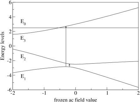
FIG. 3.: Energy level dependence on frozen ac field value (parameters see text). Arrows indicate two possible resonant excitations.

The minimum distance between the two lowest states in the avoided crossing region is $0.5$. We now expect a possible strong enhancement of the induced moments in the frequency range of the resonance indicated by the arrow $\omega\sim 5.8$ which should be most effective if the temperature is smaller than the avoided crossing splitting, i.e. $\beta~{}>~{}2$. In addition we expect to see another resonance at frequencies corresponding to the smallest splitting between the two lowest lying states, i.e. around $\omega=0.5$.

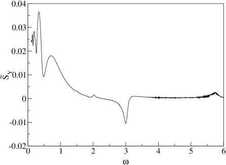
FIG. 4.: $\tilde{S}_{y}$ as function of $\omega$. Chosen parameters are: $h_{0}=3.0$, $\phi=\frac{\pi}{4}$, $\beta=10.0$, $\nu=0.1$, $J_{x}=J_{y}=5.0$ and $J_{z}=0.0$. In this case $h(t)=\sqrt{2}\cos(\omega t)$.

In Fig.4 the results of numerical simulation for $\tilde{S}_{y}$ are shown for $\beta=10$ and $\nu=0.1$. We do not observe a strong response at the expected frequency value 5.8, but we do observe in addition to the standard response at $\omega=h_{0}=3$ a response at $\omega\approx 0.5$ which corresponds to the resonant excitation in the region of the narrow avoided crossing in Fig.3. The value of $I_{NL}$ is already pretty large here, of the order of 7%.

In order to enhance the response at $\omega\approx 5.8$, we decrease the value for the dissipation constant by two orders of magnitude to $\nu=10^{-3}$. The resulting curve is shown in Fig.5. We clearly find a strong enhancement of the resonance at $\omega\approx 5.8$. In this case the value of $I_{NL}\approx 18\%$, which is the largest value we achieved to find. To characterize the dependence of this strong resonance on the parameters $\beta$ and $\nu$ we plot different curves for additional values of $\nu$ (Fig. 6) and $\beta$ (Fig. 7). The dependence on the inverse temperature shows the expected saturation at low temperatures. The dependence on $\nu$ shows a surprising non-monotonic behaviour. While it would be tempting to discuss it in terms of so-called stochastic resonance, we think that a much simpler explanation is due to the fact that in the limit of zero dissipation time reversal symmetry (12) will be restored. Consequently in the limit $\nu\rightarrow 0$ the values of the $y$-component of the induced dc magnetic moment will vanish for all frequencies.

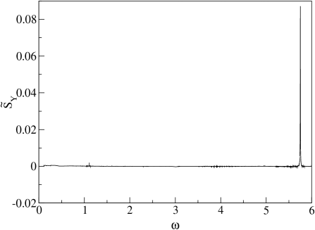
FIG. 5.: $\tilde{S}_{y}$ as function of $\omega$. Parameters as in Fig.4 except $\nu=10^{-3}$

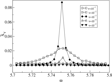
FIG. 6.: $\tilde{S}_{y}$ versus $\omega$ in the strong resonance region $\omega\approx 5.8$ for different values of $\nu$. Other parameters as in Fig.4.

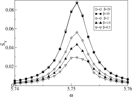
FIG. 7.: $\tilde{S}_{y}$ versus $\omega$ in the strong resonance region $\omega\approx 5.8$ for different values of $\beta$. Other parameters as in Fig.4 except $\nu=10^{-3}$.

V Conclusion

In conclusion we would like to stress once again that strong AC magnetic fields may generate zeroth harmonics in a spin system. This effect has resonant behaviour as a function of the AC field frequency and could be a new tool for the spectroscopic study of magnetic systems.

We have shown that the induction of a dc magnetic moment perpendicular to applied magnetic fields can be significantly enhanced for systems of interacting spin pairs as compared to single spins. This enhancement of the nonadiabatic nonlinear response effect is due to the presence of additional energy levels in a spin pair system, which allows to obtain additional avoided crossings between levels upon applying external fields. These avoided crossings strongly contribute to the nonlinear response through the dramatic change of wavefunctions as one sweeps through such a crossing. The presence of avoided crossings is typically associated with chaos and nonintegrability in corresponding classical systems. The case of isotropic exchange reduces the system to a single spin one and consequently does not lead to a strong enhancement of the induced moments.

The particular case of two interacting spins could be realized in stable biradicals, which provides us with the system of two spins located on the same molecule. Experimental possibility of observation of the above effect could be connected with diluted paramagnetic media at very low temperature, because only at low temperature the rate of dissipation of energy $\nu$ may become very small, thus, preventing the heating up of the system and narrowing the width of resonance, which is very important for the observation.

Other candidates for such an observation are dielectric glasses based on $SiO_{x}$. The low temperature properties of such glasses are connected with the existence of systems of double-well tunnel centers. The dynamics of these tunnel centers maps exactly onto the dynamics of spin systems. Thus, under the action of an AC electric field a permanent polarisability component could be induced. Again low temperatures are a key requirement for the observation of this effect.

Acknowledgements
We thank M. V. Fistul for helpful discussions and a critical reading of the manuscript. This work was supported by the Deutsche Forschungsgemeinschaft FL200/8-1.

REFERENCES

- [1] F. Bloch ,Phys. Rev. 102, 104 (1956)
- [2] N. Bloembergen, Nonlinear optics W. A. Benjamin Inc., (1965)
- [3] P. N. Butcher and D. Cotter, The elements of nonlinear optics Cambridge University Press, (1991)
- [4] D. G. Cory et al, Fortschritte der Physik 48, 875 (2000)
- [5] S. Flach, O. Yevtushenko, and Y. Zolotaryuk, Phys. Rev. Lett. 84, 2358 (2000)
- [6] O. Yevtushenko, S. Flach, Y. Zolotaryuk, and A. A. Ovchinnikov, Europhys. Lett. 54, 141 (2001)
- [7] S. Flach and A. A. Ovchinnikov, Physica A 292,268 (2001)