Decoherence on Grover’s quantum algorithm:
perturbative approach

Abstract

In this paper, we study decoherence on Grover’s quantum searching algorithm using a perturbative method. We assume that each two-state system (qubit) suffers $\sigma_{z}$ error with probability $p$ ($0\leq p\leq 1$) independently at every step in the algorithm. Considering an $n$-qubit density operator to which Grover’s operation is applied $M$ times, we expand it in powers of $2Mnp$ and derive its matrix element order by order under the $n\rightarrow\infty$ limit. (In this large $n$ limit, we assume $p$ is small enough, so that $2Mnp(\geq 0)$ can take any real positive value or $0$.) This approach gives us an interpretation about creation of new modes caused by $\sigma_{z}$ error and an asymptotic form of an arbitrary order correction. Calculating the matrix element up to the fifth order term numerically, we investigate a region of $2Mnp$ (perturbative parameter) where the algorithm finds the correct item with a threshold of probability $P_{\mbox{\scriptsize th}}$ or more. It satisfies $2Mnp<(8/5)(1-P_{\mbox{\scriptsize th}})$ around $2Mnp\simeq 0$ and $P_{\mbox{\scriptsize th}}\simeq 1$, and this linear relation is applied to a wide range of $P_{\mbox{\scriptsize th}}$ approximately. This observation is similar to a result obtained by E. Bernstein and U. Vazirani concerning accuracy of quantum gates for general algorithms. We cannot investigate a quantum to classical phase transition of the algorithm, because it is outside the reliable domain of our perturbation theory.

1 Introduction

Since the idea of quantum computation appeared [1][2][3], a lot of researchers have been investigating its properties, algorithms, and implementations [4][5]. A quantum computer can be thought a sequence of operations which are unitary transformations and measurements applied to two-state systems (qubits). (The qubit means a system defined on a $2$-dimensional Hilbert space $\{|0\rangle,|1\rangle\}$.) For realizing performances that conventional (classical) computer hardly shows, it makes use of the properties of quantum mechanics, such as principle of superposition and its interference, principle of uncertainty, and entanglement (quantum correlation which is stronger than classical one).

One of the most serious problem for realizing quantum computation is decoherence, which is caused by an interaction between the system of quantum computer and an environment that surrounds it [6][7]. It is pointed out that quantum information stored as a quantum state is fragile and collapses at ease by this disturbance. To investigate it, some decoherence processes are assumed and their effects on quantum algorithms are estimated [8][9]. For overcoming these troubles, quantum error-correcting codes are proposed and their availability is examined [10][11].

Not only for practical purposes but also for theoretical interests, it is an important question how robust the quantum algorithm is against this disturbance. We can expect that the quantum computer loses its efficiency gradually as decoherence gets stronger. Some researchers regard it as a quantum to classical phase transition [12].

Grover’s algorithm is considered to be an efficient amplitude amplification process for quantum states, so that it is often called a searching algorithm [13][14]. By applying the same unitary transformation to the state in iteration and amplifying an amplitude of one basis vector that we want gradually, Grover’s algorithm picks up it from a uniform superposition of $2^{n}$ basis vectors with certain probability by $O(2^{n/2})$ steps. Because it handles a general problem (an unsorted database search), it can be formulated as an oracle problem, and it is proved that its efficiency is optimal in view of computational time (the number of queries for the oracle) [14][15], many researchers have analysed this algorithm precisely and proposed a lot of applications [16].

In this paper, we study the decoherence on Grover’s quantum algorithm with a perturbative method. We assume a simple model and investigate it for higher order perturbation (numerically up to the fifth order correction), under the limit of an infinite number of qubits.

The model has the following three characteristics. First, in the Grover’s algorithm, we assume that we search the basis vector of $|0\cdots 0\rangle$ from the uniform superposition of the $n$-qubit logical basis. This assumption simplifies the iterated transformation. Second, we assume each qubit interacts with the environment independently and suffers a phase damping which causes $\sigma_{z}$ error with probability $p$ and does nothing with probability $(1-p)$ [17]. Third, we take the limit of $n\rightarrow\infty$, so that the matrix element of the density operator is simplified.

In our perturbation theory, we expand an $n$-qubit density operator to which Grover’s operation is applied $M$ times in powers of $2Mnp$ [18]. Investigating higher order terms of the perturbation, we obtain a physical interpretation that the $\sigma_{z}$ error creates new modes as the algorithm goes steps. When we take the large $n$ limit mentioned above, we assume $p$ is small enough, so that a perturbative parameter $2Mnp$ can take any positive value or $0$. Taking the $n\rightarrow\infty$ limit simplifies the matrix element of the density operator and gives us an asymptotic form of an arbitrary order term.

Calculating the matrix element up to the fifth order term numerically, we investigate a range of $2Mnp$ where the algorithm finds the correct item with a threshold of probability $P_{\mbox{\scriptsize th}}$ or more. It satisfies $2Mnp<(8/5)(1-P_{\mbox{\scriptsize th}})$ around $2Mnp\simeq 0$ and $P_{\mbox{\scriptsize th}}\simeq 1$, and this linear relation can be approximately applied to a wide range of $P_{\mbox{\scriptsize th}}$. Hence, if we fix $P_{\mbox{\scriptsize th}}$ to a certain value ($P_{\mbox{\scriptsize th}}=1/2$, for example), we have to suppress the error rate to a value which is in proportion to the inverse of the number of quantum gates.

Similar results are obtained by E. Bernstein and U. Vazirani in the study of accuracy for quantum gates [3]. They consider a quantum circuit where each quantum gate has a constant error because of inaccuracy, so it is an error of a unitary transformation and it never causes dissipation to the quantum computer. They estimate inaccuracy $\epsilon$ for which the quantum algorithm is available against the fixed number of time steps $T$, and obtain $2T\epsilon<1-P_{\mbox{\scriptsize th}}$. If we regard $p/2$ as inaccuracy $\epsilon$, and $2Mn$ as the number of whole steps in algorithm $T$, it is similar to our observations except for a factor.

A. Barenco et al. study the approximate quantum Fourier transformation (AQFT) and its decoherence [9]. Although motivation is slightly different from E. Bernstein and U. Vazirani’s, we can think their model to be the quantum Fourier transformation (QFT) with inaccurate phase gates. They confirmed that AQFT can make a performance that is not so worse than QFT’s one.

This article is arranged as follows. In Section 2, we describe the model that we analyse in this paper. In Section 3, we formulate a perturbation theory for our model and explain physical quantities that we estimate. In Section 4, we derive the matrix element of the density operator of the quantum computer for the $0$-th and first order. We give a physical interpretation about creation of new modes by $\sigma_{z}$ errors in Section 5. Then, we derive the second order correction of the matrix element in Section 6. In Section 7, we take the limit of an infinite number of qubits and give the asymptotic form of an arbitrary order term. In Section 8, we carry out numerical calculations of physical quantities up to the fifth order correction. In Section 9, we give brief discussions concerned with our results. We collect formulas for deriving matrix elements in Appendix A, and give some notes about numerical calculations of higher order perturbative terms in Appendix B.

2 Model of decoherence

In this section, we describe a model that we analyse. It is a quantum process of Grover’s algorithm which suffers a phase error in iteration.

At first, we give a brief review of Grover’s algorithm [13]. Starting from the $n$-qubit ($n\geq 2$) uniform superposition on a logical basis,

$$W|0\cdots 0\rangle=\frac{1}{\sqrt{2^{n}}}\sum_{x\in\{0,1\}^{n}}|x\rangle,$$ (1)

it increases gradually an amplitude of a certain basis vector $|x_{0}\rangle$ ($x_{0}\in\{0,1\}^{n}$) which is indicated by a quantum oracle. An operator $W$ in Eq. (1) is an $n$-fold product of a one-qubit unitary transformation (Hadamard transformation) and given by $W=H^{\otimes n}$, where

$$H=H^{\dagger}=\frac{1}{\sqrt{2}}\bordermatrix{&\langle 0|&\langle 1|\cr|0\rangle&1&1\cr|1\rangle&1&-1\cr},\quad\quad H^{\dagger}H=\mbox{\boldmath$I$}.$$ (2)

The quantum oracle can be regarded as a black box, and actually it is a quantum gate which shifts phases of logical basis vectors as

$$R_{x_{0}}:\quad\left\{\begin{array}[]{llll}|x_{0}\rangle&\rightarrow&-|x_{0}\rangle&\\ |x\rangle&\rightarrow&|x\rangle&\mbox{for $x\neq x_{0}$}\end{array}\right.,$$ (3)

where $x_{0},x\in\{0,1\}^{n}$, $R_{x_{0}}^{\dagger}=R_{x_{0}}$, and $R_{x_{0}}^{\dagger}R_{x_{0}}=\mbox{\boldmath$I$}$.

To let probability of observing $|x_{0}\rangle$ be greater than a certain value ($1/2$, for example), we repeat the following procedure $O(\sqrt{2^{n}})$ times.

1. Apply $R_{x_{0}}$ to the $n$-qubit state.

2. Apply $D=WR_{0}W$ to the $n$-qubit state.

$R_{0}$ is a selective phase shift operator which multiplies a factor $(-1)$ to $|0\cdots 0\rangle$ and does nothing to the other basis vectors, as defined in Eq. (3). $D$ is called the inversion about average operation.

From now on, we assume that we amplify an amplitude of $|0\cdots 0\rangle$. From this assumption, we can write an operation iterated in the algorithm as

$$DR_{0}=(WR_{0}W)R_{0}.$$ (4)

After repeating this operation $M$ times from the initial state of $W|0\rangle$($=W|0\cdots 0\rangle$), we obtain the state of $(WR_{0})^{2M}W|0\rangle$. (We often write $|0\rangle$ as an abbreviation of the $n$-qubit state $|0\cdots 0\rangle$ for a simple notation.)

Next, we think about the decoherence. In this paper, we consider the following one-qubit phase error [17],

$$\rho\rightarrow\rho^{\prime}=p\sigma_{z}\rho\sigma_{z}+(1-p)\rho\quad\quad\mbox{for $0\leq p\leq 1$},$$ (5)

where $\rho$ is an arbitrary one-qubit density operator and $\sigma_{z}$ is one of the Pauli matrices given by

$$\sigma_{z}=\sigma_{z}^{\dagger}=\bordermatrix{&\langle 0|&\langle 1|\cr|0\rangle&1&0\cr|1\rangle&0&-1\cr}.$$ (6)

For simplicity, we assume that the phase error of Eq. (5) occurs in each qubit of the state independently before every $R_{0}$ operation during the algorithm. It assumes that each qubit interacts with its environment and suffers the phase error independently.

Here, we add some notes. First, because $R_{0}\in U(2^{n})$ is applied to all $n$ qubits and $H\in U(2)$ is applied to only one qubit, we can imagine that the realization of $R_{0}$ is more difficult than that of $W=H^{\otimes n}$. Hence, we assume that the phase error occurs only before $R_{0}$. Second, although we assume a very simple error defined in Eq. (5), we can think other complicated errors. For example, we can consider a phase error caused by an interaction between the environment and two qubits, and it may occur with probability of $O(p^{2})$. In this paper, we do not assume such complicated errors. We discuss how the disturbance of Eq. (5) occurs in Section 9.2.

3 The perturbative method

Let $\rho^{(M)}$ be the density matrix which is obtained by applying Grover’s operation $M$ times to the $n$-qubit initial state $W|0\rangle$. The decoherence of Eq. (5) occurs $2Mn$ times in $\rho^{(M)}$. We can expand $\rho^{(M)}$ in powers of $p$ and $(1-p)$ as follows,

$$\rho^{(M)} = (1-p)^{2Mn}T_{0}^{(M)}+(1-p)^{2Mn-1}pT_{1}^{(M)}+\cdots$$ (7)

$$= \sum_{h=0}^{2Mn}(1-p)^{2Mn-h}p^{h}T_{h}^{(M)},$$

where $\{T_{h}^{(M)}\}$ are given by

$$T_{0}^{(M)} = (WR_{0})^{2M}W|0\rangle\langle 0|W(R_{0}W)^{2M},$$ (8)

$$T_{1}^{(M)} = \sum_{i=1}^{n}\sum_{k=0}^{2M-1}(WR_{0})^{2M-k}\sigma_{z}^{(i)}(WR_{0})^{k}W|0\rangle\langle 0|W(R_{0}W)^{k}\sigma_{z}^{(i)}(R_{0}W)^{2M-k},$$ (9)

$$T_{2}^{(M)} = \sum_{i=1}^{n}\sum_{{j=1}\atop{i<j}}^{n}\sum_{k=0}^{2M-1}(WR_{0})^{2M-k}\sigma_{z}^{(i)}\sigma_{z}^{(j)}(WR_{0})^{k}W|0\rangle\langle\mbox{h.c.}|$$ (10)

$$+\sum_{i=1}^{n}\sum_{j=1}^{n}\sum_{k=0}^{2M-1}\sum_{l=1}^{2M-k-1}(WR_{0})^{2M-k-l}\sigma_{z}^{(i)}(WR_{0})^{l}\sigma_{z}^{(j)}(WR_{0})^{k}W|0\rangle\langle\mbox{h.c.}|,$$

and so on, $\sigma_{z}^{(i)}$ represents the operator applied to the $i$-th qubit ($1\leq i\leq n$), and $\langle\mbox{h.c.}|$ represents a hermitian conjugation of the ket vector on its left side. We can regard $T_{h}^{(M)}$ as a density operator whose trace is not normalised. It represents states where $h$ errors occur during the iteration of $M$ operations.

On the other hand, we expand $\rho^{(M)}$ in powers of $p$ as follows,

$$\rho^{(M)} = \rho_{0}^{(M)}+2Mnp\rho_{1}^{(M)}+\frac{1}{2}(2Mn)(2Mn-1)p^{2}\rho_{2}^{(M)}+\cdots$$ (11)

$$= \sum_{h=0}^{2Mn}{2Mn\choose{h}}p^{h}\rho_{h}^{(M)},$$

where

$$\rho_{0}^{(M)} = T_{0}^{(M)},$$

$$\rho_{1}^{(M)} = -T_{0}^{(M)}+\frac{T_{1}^{(M)}}{2Mn},$$

$$\rho_{h}^{(M)} = (-1)^{h}\sum_{j=0}^{h}(-1)^{j}{2Mn\choose{j}}^{-1}{h\choose{j}}T_{j}^{(M)}\quad\quad\mbox{for $h=0,1,\cdots,2Mn$}.$$ (12)

In Section 7, we take a large $n$ limit (the limit of an infinite number of qubits). If $2Mnp$ is small enough, we can consider the series of Eq. (11) to be a perturbative expansion. Because we divide $T_{h}^{(M)}$ by $(Mn)^{h}$ as Eq. (12), an expectation value of $\rho_{h}^{(M)}$ ($h=0,1,\cdots,2Mn$) can converge on a finite value in the limit of $n\rightarrow\infty$.

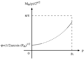
Figure 1: Variation of $M_{\mbox{\scriptsize th}}(p)/\sqrt{2^{n}}$ against $p$ with the threshold probability $P_{\mbox{\scriptsize th}}$ under large but finite $n$.

With these preparations, we will investigate the following physical quantities. Let $P_{\mbox{\scriptsize th}}$ be a threshold of probability ($0<P_{\mbox{\scriptsize th}}\leq 1$), so that if the quantum computer finds the item that we want (in our model, it is $|0\rangle$) with the probability $P_{\mbox{\scriptsize th}}$ or more, we regard it available, and otherwise we do not consider it available. Then, we consider the least number of the operations that we need to repeat for amplifying the probability of observing $|0\rangle$ to $P_{\mbox{\scriptsize th}}$ or more for given $p$. We can describe it as $M=M_{\mbox{\scriptsize th}}(p;P_{\mbox{\scriptsize th}})$, and it satisfies $\langle 0|\rho^{(M)}|0\rangle=P_{\mbox{\scriptsize th}}$. (For convenience, we write it as $M_{\mbox{\scriptsize th}}(p)$ with omitting $P_{\mbox{\scriptsize th}}$ as far as it does not make confusion.) Because of

$$\langle 0|T_{0}^{(M)}|0\rangle_{p=0}\simeq\sin^{2}(2M/\sqrt{2^{n}})\quad\quad\mbox{for large but finite $n$},$$ (13)

obtained in Section 4, $M_{\mbox{\scriptsize th}}(p)$ takes a value of $\varphi\sqrt{2^{n}}$ at $p=0$ (with no decoherence) for large finite $n$, where $\varphi=(1/2)\arcsin\sqrt{P_{\mbox{\scriptsize th}}}$.

As $p$ gets larger, we can expect that $M_{\mbox{\scriptsize th}}(p)$ increases monotonously. It could be possible for certain $p_{\mbox{\scriptsize c}}$ or more that we never observe $|0\rangle$ at least with probability of $P_{\mbox{\scriptsize th}}$. (Hence, $p_{\mbox{\scriptsize c}}$ depends on $P_{\mbox{\scriptsize th}}$.) Such behaviour of $M_{\mbox{\scriptsize th}}(p)$ can be drawn in Figure 1. We multiply a factor $1/\sqrt{2^{n}}$ to $M_{\mbox{\scriptsize th}}(p)$ for normalisation. Because $\langle 0|\rho^{(M)}|0\rangle$ with $p=0$ increases monotonously from $M=0$ to $M=(\pi/4)\sqrt{2^{n}}$ and then decreases as shown in Eq. (13), $M_{\mbox{\scriptsize th}}(p)/\sqrt{2^{n}}$ at $p=p_{\mbox{\scriptsize c}}$ is equal to or less than $\pi/4$.

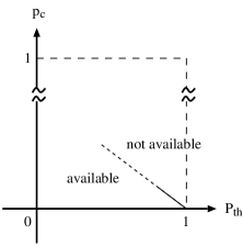
Figure 2: Variation of $p_{\mbox{\scriptsize c}}$ against $P_{\mbox{\scriptsize th}}$.

Regarding $P_{\mbox{\scriptsize th}}$ as a threshold whether the quantum computer is available or not, we can consider $p_{\mbox{\scriptsize c}}$ to be a critical point. (This is not a so-called quantum to classical phase transition.) We can draw a graph of $p_{\mbox{\scriptsize c}}$ against $P_{\mbox{\scriptsize th}}$ as Figure 2. (If $P_{\mbox{\scriptsize th}}=1$, we obtain $p_{\mbox{\scriptsize c}}=0$.)

In this paper, we calculate physical quantities using the perturbative parameter $x=2Mnp$, so that we take $M/\sqrt{2^{n}}$ and $x$ for independent variables. (In our original model defined in Section 2, we take $M$ and $p$ for independent variables.) We can define as well $\tilde{M}_{\mbox{\scriptsize th}}(x;P_{\mbox{\scriptsize th}})/\sqrt{2^{n}}$ that represents the least number of the operations iterated for amplifying the probability of $|0\rangle$ to $P_{\mbox{\scriptsize th}}$ for given $x$. Furthermore, we also obtain $x_{c}$, for which or more we can never detect $|0\rangle$ at least with probability $P_{\mbox{\scriptsize th}}$. Hence, we obtain a graph of $\tilde{M}_{\mbox{\scriptsize th}}(x)/\sqrt{2^{n}}$ versus $x$ instead of Figure 1, and that of $x_{\mbox{\scriptsize c}}$ versus $P_{\mbox{\scriptsize th}}$ instead of Figure 2. The differences of these quantities are discussed in Section 8.

The dependence of $x_{\mbox{\scriptsize c}}$ on $P_{\mbox{\scriptsize th}}$ gives us useful information. If we regard $2Mn$ as the number of computational steps $T$, and $p/2$ as a parameter $\epsilon$ which represents a degree of errors, it serves the region of $T\epsilon$ where the quantum computer is available for $P_{\mbox{\scriptsize th}}$, because of $x=2Mnp$. To make these analyses, we need to know $\langle 0|\rho^{(M)}|0\rangle$. In the following sections, we calculate $\langle 0|\rho^{(M)}|0\rangle$ to the fifth order of $p$ (up to $(2Mnp)^{5}$) numerically under the $n\rightarrow\infty$ limit.

4 Matrix elements up to the first order

In this section, we consider matrix elements of the density operators with no and one error, $\langle 0|T_{0}^{(M)}|0\rangle$ and $\langle 0|T_{1}^{(M)}|0\rangle$, defined in Eqs. (8) and (9).

First, we derive $T_{0}^{(M)}$ and $\langle 0|T_{0}^{(M)}|0\rangle$. Using Eq. (108) in Appendix A.1, we obtain

$$T_{0}^{(M)}=[\sin(2M+1)\theta|0\rangle+\frac{\cos(2M+1)\theta}{\sqrt{2^{n}-1}}\sum_{x\neq 0}|x\rangle]\langle\mbox{h.c.}|,$$ (14)

$$\langle 0|T_{0}^{(M)}|0\rangle=\sin^{2}(2M+1)\theta,$$ (15)

where

$$\sin\theta=\frac{1}{\sqrt{2^{n}}},\quad\quad\cos\theta=\sqrt{\frac{2^{n}-1}{2^{n}}}.$$ (16)

(This parameter $\theta$ is introduced by M. Boyer et al. and it simplifies our notation [14].) From Eq. (15), we notice the following facts. If there is no decoherence ($p=0$), we can amplify probability of observing $|0\rangle$ to unity. Taking large (but finite) $n$, we obtain $\sin\theta\simeq\theta$ and $\theta\simeq 1/\sqrt{2^{n}}$, and we can observe $|0\rangle$ with probability of unity after repeating Grover’s operation $M_{\mbox{\scriptsize max}}\simeq(\pi/4)\sqrt{2^{n}}$ times.

Then, we think about $T_{1}^{(M)}$ and $\langle 0|T_{1}^{(M)}|0\rangle$. For convenience, in spite of the definition of $T_{1}^{(M)}$ given in Eq. (9), we rewrite it as follows,

$$T_{1}^{(M)} = \sum_{i=1}^{n}\sum_{k=0}^{M-1}(WR_{0})^{2(M-k)}\sigma_{z}^{(i)}(WR_{0})^{2k}W|0\rangle\langle\mbox{h.c.}|$$ (17)

$$+\sum_{i=1}^{n}\sum_{k=0}^{M-1}(WR_{0})^{2(M-k)-1}\sigma_{z}^{(i)}(WR_{0})^{2k+1}W|0\rangle\langle\mbox{h.c.}|.$$

We can derive an explicit form of $\langle 0|T_{1}^{(M)}|0\rangle$ using formulas collected in Appendixes A.1 and A.2. The matrix element of the first term in Eq. (17) can be given by $|{\cal T}_{\mbox{\scriptsize even}}^{(k)}|^{2}$, where

$${\cal T}_{\mbox{\scriptsize even}}^{(k)} \equiv \langle 0|(WR_{0})^{2(M-k)}\sigma_{z}^{(i)}(WR_{0})^{2k}W|0\rangle$$ (18)

$$= (-1)^{M-k}[\cos 2(M-k)\theta\langle 0|+\frac{\sin 2(M-k)\theta}{\sqrt{2^{n}-1}}\sum_{x\neq 0}\langle x|]\sigma_{z}^{(i)}$$

$$\times(-1)^{k}[\sin(2k+1)\theta|0\rangle+\frac{\cos(2k+1)\theta}{\sqrt{2^{n}-1}}\sum_{y\neq 0}|y\rangle]$$

$$= (-1)^{M}[\cos 2(M-k)\theta\sin(2k+1)\theta-\frac{1}{2^{n}-1}\sin 2(M-k)\theta\cos(2k+1)\theta].$$

We notice that ${\cal T}_{\mbox{\scriptsize even}}^{(k)}$ does not depend on the subscript $i$. In a similar way, we can obtain a matrix element of the second term in Eq. (17) as $|{\cal T}_{\mbox{\scriptsize odd}}^{(k)}|^{2}$, where

$${\cal T}_{\mbox{\scriptsize odd}}^{(k)} \equiv \langle 0|(WR_{0})^{2(M-k)-1}\sigma_{z}^{(i)}(WR_{0})^{2k+1}W|0\rangle$$ (19)

$$= (-1)^{M}[\sin(2M-2k-1)\theta\cos 2(k+1)\theta-\frac{1}{2^{n}-1}\cos(2M-2k-1)\theta\sin 2(k+1)\theta].$$

(Here, we notice $|{\cal T}_{\mbox{\scriptsize even}}^{(k)}|^{2}=|{\cal T}_{\mbox{\scriptsize odd}}^{(M-k-1)}|^{2}$.) Hence, we obtain

$$\langle 0|T_{1}^{(M)}|0\rangle=n\sum_{k=0}^{M-1}(|{\cal T}_{\mbox{\scriptsize even}}^{(k)}|^{2}+(|{\cal T}_{\mbox{\scriptsize odd}}^{(k)}|^{2}).$$ (20)

5 Physical interpretation for creation of modes

If we derive the explicit form of $T_{1}^{(M)}$, we can obtain a physical interpretation of creating modes by $\sigma_{z}$ error.

Let us consider the state included in Eq. (17),

$$(WR_{0})^{l}\sigma_{z}^{(i)}(WR_{0})^{k}W|0\rangle,$$ (21)

which suffers the phase error only once. From Eq. (108) in Appendix A.1, we obtain the following equation,

$$\sigma_{z}^{(i)}(WR_{0})^{2k}W|0\rangle$$ (22)

$$= (-1)^{k}[\sin(2k+1)\theta|0\rangle+\frac{\cos(2k+1)\theta}{\sqrt{2^{n}-1}}(\sum_{{x\neq 0}\atop{x_{i}=0}}|x\rangle-\sum_{{x\neq 0}\atop{x_{i}=1}}|x\rangle)]$$

$$= (WR_{0})^{2k}W|0\rangle-\sqrt{2}(-1)^{k}\frac{\cos(2k+1)\theta}{\cos\theta}|\eta_{i}\rangle\quad\quad\mbox{for $k=0,1,\cdots$},$$

where

$$|\eta_{i}\rangle=\frac{1}{\sqrt{2^{n-1}}}\sum_{x_{i}=1}|x\rangle\quad\quad\mbox{for $i=1,\cdots,n$}.$$ (23)

In a similar way, from Eq. (109), we obtain

$$\sigma_{z}^{(i)}(WR_{0})^{2k+1}W|0\rangle=(WR_{0})^{2k+1}W|0\rangle+\sqrt{2}(-1)^{k}\frac{\sin 2(k+1)\theta}{\cos\theta}|\eta_{i}\rangle\quad\quad\mbox{for $k=0,1,\cdots$}.$$ (24)

To obtain an explicit form of Eq. (21), we have to apply $WR_{0}$ to Eqs. (22) and (24) from the left side step by step. (We count $WR_{0}$ as one step for a while.) We can derive an explicit form of $(WR_{0})^{l}|\eta_{i}\rangle$ as follows. In the case of $l=1$, we obtain

$$WR_{0}|\eta_{i}\rangle=\frac{1}{\sqrt{2}}(|0\rangle-|\overline{i}\rangle),$$ (25)

where $\overline{i}$ represents a binary string whose all digits are ‘$0$’ but the $i$-th digit is ‘$1$’, so that

$$|\overline{i}\rangle=|0\cdots 0\begin{array}[t]{c}1\\ \uparrow\\ i\end{array}0\cdots 0\rangle.$$ (26)

For $l=2$, we obtain

$$(WR_{0})^{2}|\eta_{i}\rangle = \frac{1}{\sqrt{2}}WR_{0}(|0\rangle-|\overline{i}\rangle)$$ (27)

$$= -\frac{1}{\sqrt{2^{n-1}}}\sum_{x_{i}=0}|x\rangle$$

$$= -\sqrt{2}W|0\rangle+|\eta_{i}\rangle.$$

Therefore, we obtain

$$(WR_{0})^{2l}|\eta_{i}\rangle = -\sqrt{2}\sum_{m=0}^{l-1}(WR_{0})^{2m}W|0\rangle+|\eta_{i}\rangle\quad\quad\mbox{for $l=0,1,\cdots$},$$ (28)

$$(WR_{0})^{2l+1}|\eta_{i}\rangle = -\sqrt{2}\sum_{m=0}^{l-1}(WR_{0})^{2m+1}W|0\rangle+\frac{1}{\sqrt{2}}(|0\rangle-|\overline{i}\rangle)\quad\quad\mbox{for $l=0,1,\cdots$},$$ (29)

where $\sum_{l=0}^{-1}$ means that no term is summed up.

From Eqs. (22), (24), (28), and (29), we can describe $(WR_{0})^{l}\sigma_{z}^{(i)}(WR_{0})^{k}W|0\rangle$ for $k=0,1,\cdots$ and $l=1,2,\cdots$ with $(WR_{0})^{k}W|0\rangle$, $|\eta_{i}\rangle$, and $(|0\rangle-|\overline{i}\rangle)$. (We obtain the explicit form of $(WR_{0})^{k}W|0\rangle$ in Appendix A.1.) For example, we can write

$$(WR_{0})^{2l}\sigma_{z}^{(i)}(WR_{0})^{2k}W|0\rangle$$ (30)

$$= (WR_{0})^{2(k+l)}W|0\rangle-\sqrt{2}(-1)^{k}\frac{\cos(2k+1)\theta}{\cos\theta}[-\sqrt{2}\sum_{m=0}^{l-1}(WR_{0})^{2m}W|0\rangle+|\eta_{i}\rangle]$$

$$\quad\quad\mbox{for $k=0,1,\cdots$ and $l=1,2,\cdots$}.$$

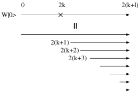
Figure 3: Creation of modes by the error.

This equation allows us the following interpretation. If $\sigma_{z}$ error occurs in the $i$-th qubit of the $n$-qubit state at the $2k$-th step, it causes new modes which are created as the initial state $W|0\rangle$ at every two steps from $2(k+1)$, that is, $2(k+1)$-th, $2(k+2)$-th, $2(k+3)$-th, $\cdots$, and so on. (See Figure 3.) The state becomes a superposition of them.

Here, we derive the matrix element $\langle 0|T_{1}^{(M)}|0\rangle$ again using this interpretation. From Eqs. (30) and (108) in Appendix A.1, we obtain

$$\langle 0|(WR_{0})^{2(M-k)}\sigma_{z}^{(i)}(WR_{0})^{2k}W|0\rangle$$ (31)

$$= \langle 0|(WR_{0})^{2M}W|0\rangle$$

$$-\sqrt{2}(-1)^{k}\frac{\cos(2k+1)\theta}{\cos\theta}[-\sqrt{2}\sum_{l=0}^{M-k-1}\langle 0|(WR_{0})^{2l}W|0\rangle+\langle 0|\eta_{i}\rangle]$$

$$= (-1)^{M}\sin(2M+1)\theta+2(-1)^{k}\frac{\cos(2k+1)\theta}{\cos\theta}\sum_{l=0}^{M-k-1}(-1)^{l}\sin(2l+1)\theta.$$

(We eliminate one $\sigma_{z}$ operator from the above equation.) Then using a formula of Eq. (112) in Appendix A.3 to sum up trigonometric functions, we can rewrite Eq. (31) as

$$\langle 0|(WR_{0})^{2(M-k)}\sigma_{z}^{(i)}(WR_{0})^{2k}W|0\rangle$$ (32)

$$= (-1)^{M}\sin(2M+1)\theta+2(-1)^{k}\frac{\cos(2k+1)\theta}{\cos\theta}\frac{(-1)^{M-k-1}}{2}\frac{\sin 2(M-k)\theta}{\cos\theta}$$

$$= (-1)^{M}[\cos 2(M-k)\theta\sin(2k+1)\theta-\frac{1}{2^{n}-1}\sin 2(M-k)\theta\cos(2k+1)\theta]$$

$$= {\cal T}_{\mbox{\scriptsize even}}^{(k)},$$

where we substitute $\cos^{2}\theta=(2^{n}-1)/2^{n}$ of Eq. (16). In this derivation, we expand the matrix elements into a series of modes by Eq. (30), and sum up them by the formula of Appendix A.3. We often use this technique in this paper.

In a similar way, using Eqs. (24), (29), (109), and (115), we obtain

$$\langle 0|(WR_{0})^{2(M-k)-1}\sigma_{z}^{(i)}(WR_{0})^{2k+1}W|0\rangle$$ (33)

$$= \langle 0|(WR_{0})^{2M}W|0\rangle$$

$$+\sqrt{2}(-1)^{k}\frac{\sin 2(k+1)\theta}{\cos\theta}[-\sqrt{2}\sum_{l=0}^{M-k-2}\langle 0|(WR_{0})^{2l+1}W|0\rangle+\frac{1}{\sqrt{2}}\langle 0|(|0\rangle-|\overline{i}\rangle)]$$

$$= (-1)^{M}\sin(2M+1)\theta+2(-1)^{k}\frac{\sin 2(k+1)\theta}{\cos\theta}[-\sum_{l=0}^{M-k-2}(-1)^{l}\cos 2(l+1)\theta+\frac{1}{2}]$$

$$= (-1)^{M}\sin(2M+1)\theta$$

$$+2(-1)^{k}\frac{\sin 2(k+1)\theta}{\cos\theta}[-\frac{1}{2}-\frac{(-1)^{M-k-2}}{2\cos\theta}\cos(2M-2k-1)\theta+\frac{1}{2}]$$

$$= {\cal T}_{\mbox{\scriptsize odd}}^{(k)}.$$

6 Matrix element of the second order

In this section, we consider the matrix element $\langle 0|T_{2}^{(M)}|0\rangle$ which contains two $\sigma_{z}$ errors, defined in Eq. (10). We make good use of the interpretation of creating new modes discussed in Section 5 for obtaining it.

Let us see the first term of Eq. (10). It suffers two $\sigma_{z}$ errors at the same step as follows,

$$\langle 0|(WR_{0})^{2M-k}\sigma_{z}^{(i)}\sigma_{z}^{(j)}(WR_{0})^{k}W|0\rangle\quad\quad\mbox{for $1\leq i\leq n$, $1\leq j\leq n$, and $i\neq j$}.$$ (34)

Here, we consider the following term,

$$\langle 0|(WR_{0})^{2(M-k)}\sigma_{z}^{(i)}\sigma_{z}^{(j)}(WR_{0})^{2k}W|0\rangle$$ (35)

$$= (-1)^{M}[\cos 2(M-k)\theta\sin(2k+1)\theta$$

$$+\frac{1}{2^{n}-1}\sin 2(M-k)\theta\cos(2k+1)\theta\sum_{x\neq 0}\sum_{y\neq 0}\langle x|\sigma_{z}^{(i)}\sigma_{z}^{(j)}|y\rangle]$$

$$\quad\quad\mbox{for $k=0,1,\cdots,M-1$},$$

where we use Eqs. (108) and (110) in Appendixes A.1 and A.2. To obtain an explicit form of the above, we have to calculate $\sum_{x\neq 0}\sum_{y\neq 0}\langle x|\sigma_{z}^{(i)}\sigma_{z}^{(j)}|y\rangle$ for $i\neq j$.

Figure 4: Relation between ${\cal S}$, ${\cal S}_{1}$, and ${\cal S}_{2}$.

For deriving it, we define a set ${\cal S}=\{|x\rangle:x\in\{0,1\}^{n},x\neq 0\}$, and its subsets, ${\cal S}_{1}=\{|x\rangle:|x\rangle\in{\cal S},x_{i}=1\}$ and ${\cal S}_{2}=\{|x\rangle:|x\rangle\in{\cal S},x_{j}=1\}$, as shown in Figure 4. The number of elements of them and ${\cal S}_{1}\cap{\cal S}_{2}$ are given as $|{\cal S}|=2^{n}-1$, $|{\cal S}_{1}|=|{\cal S}_{2}|=2^{n-1}$, and $|{\cal S}_{1}\cap{\cal S}_{2}|=2^{n-2}$. A set of basis vectors whose signs are flipped by $\sigma_{z}^{(i)}\sigma_{z}^{(j)}$ is given by $({\cal S}_{1}\cup{\cal S}_{2})\cap(\overline{{\cal S}_{1}\cap{\cal S}_{2}})$, and the number of its elements is equal to $2^{n-1}$. Hence, the number of elements in ${\cal S}$ whose signs are not flipped is equal to $(2^{n-1}-1)$. From these considerations, we obtain

$$\sum_{x\neq 0}\sum_{y\neq 0}\langle x|\sigma_{z}^{(i)}\sigma_{z}^{(j)}|y\rangle=-1,$$ (36)

and

$$\langle 0|(WR_{0})^{2(M-k)}\sigma_{z}^{(i)}\sigma_{z}^{(j)}(WR_{0})^{2k}W|0\rangle={\cal T}_{\mbox{\scriptsize even}}^{(k)}.$$ (37)

In a similar way, we can obtain

$$\langle 0|(WR_{0})^{2(M-k)-1}\sigma_{z}^{(i)}\sigma_{z}^{(j)}(WR_{0})^{2k+1}W|0\rangle={\cal T}_{\mbox{\scriptsize odd}}^{(k)}\quad\quad\mbox{for $k=0,1,\cdots,M-1$}.$$ (38)

Therefore, the matrix element of the first term in Eq. (10) is equal to $[(n-1)/2]\langle 0|T_{1}^{(M)}|0\rangle$.

Then, we think about the second term in Eq. (10). Using Eq. (30), we obtain the following term,

$${\cal T}_{\mbox{\scriptsize even},\mbox{\scriptsize even}}^{(k,l;\delta_{ij})} \equiv \langle 0|(WR_{0})^{2(M-k-l)}\sigma_{z}^{(i)}\biggl{[}(WR_{0})^{2l}\sigma_{z}^{(j)}(WR_{0})^{2k}W|0\rangle\biggr{]}$$ (39)

$$= \langle 0|(WR_{0})^{2(M-k-l)}\sigma_{z}^{(i)}(WR_{0})^{2(k+l)}W|0\rangle$$

$$-\sqrt{2}(-1)^{k}\frac{\cos(2k+1)\theta}{\cos\theta}$$

$$\times[-\sqrt{2}\sum_{m=0}^{l-1}\langle 0|(WR_{0})^{2(M-k-l)}\sigma_{z}^{(i)}(WR_{0})^{2m}W|0\rangle+\langle 0|(WR_{0})^{2(M-k-l)}\sigma_{z}^{(i)}|\eta_{j}\rangle].$$

The bracket $[\cdots]$ in the first line of Eq. (39) represents that this part is calculated at first. Here, we use the same technique in Section 5 again. We expand the matrix element by modes caused by the $\sigma_{z}$ error and sum up them. (We eliminate one $\sigma_{z}$ operator from ${\cal T}_{\mbox{\scriptsize even},\mbox{\scriptsize even}}^{(k,l;\delta_{ij})}$.) As a result of Eq. (39), we obtain terms which contains only one $\sigma_{z}$ error, and essentially they have been obtained already in Sections 4 and 5. Here, we introduce a notation of

$${\cal G}^{(1)}(k,l)=\langle 0|(WR_{0})^{l}\sigma_{z}^{(i)}(WR_{0})^{k}W|0\rangle,\quad\quad\mbox{for $k=0,1,\cdots$, $l=1,2,\cdots$},$$ (40)

and collect its explicit form in Appendix A.4. We also collect some formulas of $|\eta_{j}\rangle$ and $(|0\rangle-|\overline{j}\rangle)$ in Appendix A.5.

Using Eqs. (112), (114), (116), and (120) in Appendixes A.3, A.4, and A.5, we obtain

$${\cal T}_{\mbox{\scriptsize even},\mbox{\scriptsize even}}^{(k,l;\delta_{ij})} = {\cal G}^{(1)}(2(k+l),2(M-k-l))$$ (41)

$$-\sqrt{2}(-1)^{k}\frac{\cos(2k+1)\theta}{\cos\theta}$$

$$\times\{-\sqrt{2}\sum_{m=0}^{l-1}(-1)^{M-k-l+m}[\cos 2(M-k-l)\theta\sin(2m+1)\theta$$

$$-\frac{1}{2^{n}-1}\sin 2(M-k-l)\theta\cos(2m+1)\theta]$$

$$-\frac{(-1)^{M-k-l}}{\sqrt{2}}\frac{\sin 2(M-k-l)\theta}{\cos\theta}\delta_{ij}\}$$

$$= {\cal G}^{(1)}(2(k+l),2(M-k-l))$$

$$-(-1)^{M}\frac{\cos(2k+1)\theta}{\cos^{2}\theta}$$

$$\times\{[\cos 2(M-k-l)\theta\sin 2l\theta-\frac{1}{2^{n}-1}\sin 2(M-k-l)\theta\cos 2l\theta]$$

$$+(-1)^{-l}(\frac{1}{2^{n}-1}-\delta_{ij})\sin 2(M-k-l)\theta\}.$$

From the above, we notice that ${\cal T}_{\mbox{\scriptsize even},\mbox{\scriptsize even}}^{(k,l;\delta_{ij})}$ depends on $\delta_{ij}$ (and not on $i$ and $j$).

As results of similar considerations, using Eqs. (22), (24), (28), (29), and formulas in Appendixes A.3, A.4, and A.5, we obtain the other matrix elements,

$${\cal T}_{\mbox{\scriptsize odd},\mbox{\scriptsize even}}^{(k,l;\delta_{ij})} \equiv \langle 0|(WR_{0})^{2(M-k-l)-1}\sigma_{z}^{(i)}(WR_{0})^{2l}\sigma_{z}^{(j)}(WR_{0})^{2k+1}W|0\rangle$$ (42)

$$= {\cal G}^{(1)}(2(k+l)+1,2(M-k-l)-1)$$

$$+(-1)^{M}\frac{\sin 2(k+1)\theta}{\cos^{2}\theta}$$

$$\times\{[\sin(2M-2k-2l-1)\theta\sin 2l\theta+\frac{1}{2^{n}-1}\cos(2M-2k-2l-1)\theta\cos 2l\theta]$$

$$+(-1)^{l-1}(\frac{1}{2^{n}-1}-\delta_{ij})\cos(2M-2k-2l-1)\theta\},$$

$${\cal T}_{\mbox{\scriptsize even},\mbox{\scriptsize odd}}^{(k,l;\delta_{ij})} \equiv \langle 0|(WR_{0})^{2(M-k-l)-1}\sigma_{z}^{(i)}\biggl{[}(WR_{0})^{2l+1}\sigma_{z}^{(j)}(WR_{0})^{2k}W|0\rangle\biggr{]}$$ (43)

$$= {\cal G}^{(1)}(2(k+l)+1,2(M-k-l)-1)$$

$$-\sqrt{2}(-1)^{k}\frac{\cos(2k+1)\theta}{\cos\theta}[-\sqrt{2}\sum_{m=0}^{l-1}{\cal G}^{(1)}(2m+1,2(M-k-l)-1)$$

$$+\frac{1}{\sqrt{2}}\langle 0|(WR_{0})^{2(M-k-l)-1}\sigma_{z}^{(i)}(|0\rangle)-|\overline{j}\rangle]\}$$

$$= {\cal G}^{(1)}(2(k+l)+1,2(M-k-l)-1)$$

$$-\sqrt{2}(-1)^{k}\frac{\cos(2k+1)\theta}{\cos\theta}$$

$$\times\{-\sqrt{2}\sum_{m=0}^{l-1}(-1)^{M-k-l-1+m}[-\sin(2M-2k-2l-1)\theta\cos 2(m+1)\theta$$

$$+\frac{1}{2^{n}-1}\cos(2M-2k-2l-1)\theta\sin 2(m+1)\theta]$$

$$-\frac{(-1)^{M-k-l-1}}{\sqrt{2}}[\sin(2M-2k-2l-1)\theta+(-1)^{\delta_{ij}}\frac{\cos(2M-2k-2l-1)\theta}{\sqrt{2^{n}-1}}]\}$$

$$= {\cal G}^{(1)}(2(k+l)+1,2(M-k-l)-1)$$

$$-(-1)^{M}\frac{\cos(2k+1)\theta}{\cos^{2}\theta}$$

$$\times\{[\sin(2M-2k-2l-1)\theta\cos(2l+1)\theta-\frac{1}{2^{n}-1}\cos(2M-2k-2l-1)\theta\sin(2l+1)\theta]$$

$$+\frac{(-1)^{l}}{\sqrt{2^{n}}}[\frac{1}{2^{n}-1}+(-1)^{\delta_{ij}}]\cos(2M-2k-2l-1)\theta\},$$

$${\cal T}_{\mbox{\scriptsize odd},\mbox{\scriptsize odd}}^{(k,l;\delta_{ij})} \equiv \langle 0|(WR_{0})^{2(M-k-l-1)}\sigma_{z}^{(i)}(WR_{0})^{2l+1}\sigma_{z}^{(j)}(WR_{0})^{2k+1}W|0\rangle$$ (44)

$$= {\cal G}^{(1)}(2(k+l)+1,2(M-k-l-1))$$

$$+(-1)^{M}\frac{\sin 2(k+1)\theta}{\cos^{2}\theta}$$

$$\times\{-[\cos 2(M-k-l-1)\theta\cos(2l+1)\theta+\frac{1}{2^{n}-1}\sin 2(M-k-l-1)\theta\sin(2l+1)\theta]$$

$$+\frac{(-1)^{l}}{\sqrt{2^{n}}}[\frac{1}{2^{n}-1}+(-1)^{\delta_{ij}}]\sin 2(M-k-l-1)\theta\}.$$

Finally, we can write $\langle 0|T_{2}^{(M)}|0\rangle$ as

$$\langle 0|T_{2}^{(M)}|0\rangle = \frac{n-1}{2}\langle 0|T_{1}^{(M)}|0\rangle$$ (45)

$$+\sum_{k=0}^{M-1}\sum_{l=1}^{M-k-1}[n(n-1)|{\cal T}_{\mbox{\scriptsize even},\mbox{\scriptsize even}}^{(k,l;0)}|^{2}+n|{\cal T}_{\mbox{\scriptsize even},\mbox{\scriptsize even}}^{(k,l;1)}|^{2}]$$

$$+\sum_{k=0}^{M-1}\sum_{l=1}^{M-k-1}[n(n-1)|{\cal T}_{\mbox{\scriptsize odd},\mbox{\scriptsize even}}^{(k,l;0)}|^{2}+n|{\cal T}_{\mbox{\scriptsize odd},\mbox{\scriptsize even}}^{(k,l;1)}|^{2}]$$

$$+\sum_{k=0}^{M-1}\sum_{l=0}^{M-k-1}[n(n-1)|{\cal T}_{\mbox{\scriptsize even},\mbox{\scriptsize odd}}^{(k,l;0)}|^{2}+n|{\cal T}_{\mbox{\scriptsize even},\mbox{\scriptsize odd}}^{(k,l;1)}|^{2}]$$

$$+\sum_{k=0}^{M-1}\sum_{l=0}^{M-k-2}[n(n-1)|{\cal T}_{\mbox{\scriptsize odd},\mbox{\scriptsize odd}}^{(k,l;0)}|^{2}+n|{\cal T}_{\mbox{\scriptsize odd},\mbox{\scriptsize odd}}^{(k,l;1)}|^{2}].$$

7 Large $n$ limit and asymptotic forms of matrix elements

The matrix elements, $\langle 0|T_{1}^{(M)}|0\rangle$ and $\langle 0|T_{2}^{(M)}|0\rangle$ obtained in Sections 4 and 6, are too complicated to handle as they are. In this section, we take the limit of an infinite number of qubits ($n\rightarrow\infty$), and discuss their asymptotic forms. We also discuss how to obtain an asymptotic form of any higher order term under $n\rightarrow\infty$.

We consider the limit of $n\rightarrow\infty$ for $n$-qubit state. We assume we can take very small $p$, so that $x=2Mnp$ can be an arbitrary real positive value or $0$. If $0\leq M<2\pi\sqrt{2^{n}}$, $M\theta$ converges on a certain value of $\Theta$ ($0\leq\Theta<2\pi$) under this limit. (The definition of $\theta$ is given in Eq. (16).) It is reasonable that we assume $M$ is order of $O(\sqrt{2^{n}})$ or less and define $\Theta\equiv\lim_{n\rightarrow\infty}M\theta$. Because $\langle 0|T_{h}^{(M)}|0\rangle/(Mn)^{h}$ does not depend on $p$, we can take $n\rightarrow\infty$ for it naively. Hence, from Eq. (15), we obtain

$$\lim_{n\rightarrow\infty}\langle 0|T_{0}^{(M)}|0\rangle=\sin^{2}2\Theta.$$ (46)

Then, we consider the asymptotic form of $\langle 0|T_{1}^{(M)}|0\rangle$ in Eqs. (18), (19), and (20). To let it converge on finite value, we divide it by a factor of $Mn$ as shown in Eq. (12). We can obtain

$$\lim_{n\rightarrow\infty}\frac{\langle 0|T_{1}^{(M)}|0\rangle}{Mn}=\lim_{n\rightarrow\infty}\frac{1}{M}\sum_{k=0}^{M-1}[|\tilde{{\cal T}}_{\mbox{\scriptsize even}}^{(k)}|^{2}+|\tilde{{\cal T}}_{\mbox{\scriptsize even}}^{(k)}|^{2}],$$ (47)

where

$$\tilde{{\cal T}}_{\mbox{\scriptsize even}}^{(k)} = (-1)^{M}\cos 2(M-k)\theta\sin(2k+1)\theta,$$

$$\tilde{{\cal T}}_{\mbox{\scriptsize odd}}^{(k)} = (-1)^{M}\sin(2M-2k-1)\theta\cos 2(k+1)\theta.$$ (48)

(We drop the terms with a factor $1/(2^{n}-1)$ in ${\cal T}_{\mbox{\scriptsize even}}^{(k)}$ and ${\cal T}_{\mbox{\scriptsize odd}}^{(k)}$, and obtain Eq.(48).) We substitute $\Theta=\lim_{n\rightarrow\infty}M\theta$, $\phi=k\theta$, and

$$\lim_{n\rightarrow\infty}\sum_{k=0}^{M-1}\theta=\int_{0}^{\Theta}d\phi$$ (49)

into Eq. (47), and obtain

$$\lim_{n\rightarrow\infty}\frac{\langle 0|T_{1}^{(M)}|0\rangle}{Mn} = \frac{1}{\Theta}\int_{0}^{\Theta}d\phi\{[\cos 2(\Theta-\phi)\sin 2\phi]^{2}+[\sin 2(\Theta-\phi)\cos 2\phi]^{2}\}$$ (50)

$$= \frac{1}{2}-\frac{1}{4}\cos 4\Theta-\frac{1}{16\Theta}\sin 4\Theta.$$

Next, we consider an asymptotic form of $\langle 0|T_{2}^{(M)}|0\rangle$ obtained in Eqs. (41), (42), (43), (44), and (45). Because of convergence, we divide it by $(Mn)^{2}$ as Eq. (12). In the limit of $n\rightarrow\infty$, we can neglect $\langle 0|T_{1}^{(M)}|0\rangle$ and ${\cal T}_{\alpha,\beta}^{(k,l;1)}$ for $\alpha,\beta\in\{\mbox{even},\mbox{odd}\}$, and we obtain

$$\lim_{n\rightarrow\infty}\frac{\langle 0|T_{2}^{(M)}|0\rangle}{(Mn)^{2}} = \lim_{n\rightarrow\infty}\frac{1}{M^{2}}[\sum_{k=0}^{M-1}\sum_{l=1}^{M-k-1}|\tilde{{\cal T}}_{\mbox{\scriptsize even},\mbox{\scriptsize even}}^{(k,l;0)}|^{2}+\sum_{k=0}^{M-1}\sum_{l=1}^{M-k-1}|\tilde{{\cal T}}_{\mbox{\scriptsize odd},\mbox{\scriptsize even}}^{(k,l;0)}|^{2}$$ (51)

$$+\sum_{k=0}^{M-1}\sum_{l=0}^{M-k-1}|\tilde{{\cal T}}_{\mbox{\scriptsize even},\mbox{\scriptsize odd}}^{(k,l;0)}|^{2}+\sum_{k=0}^{M-1}\sum_{l=0}^{M-k-2}|\tilde{{\cal T}}_{\mbox{\scriptsize odd},\mbox{\scriptsize odd}}^{(k,l;0)}|^{2}],$$

where

$$\tilde{{\cal T}}_{\mbox{\scriptsize even},\mbox{\scriptsize even}}^{(k,l;0)} = (-1)^{M}[\cos 2(M-k-l)\theta\sin(2k+2l+1)\theta$$

$$-\cos(2k+1)\theta\cos 2(M-k-l)\theta\sin 2l\theta]$$

$$= (-1)^{M}\cos 2(M-k-l)\theta\cos 2l\theta\sin(2k+1)\theta,$$

$$\tilde{{\cal T}}_{\mbox{\scriptsize odd},\mbox{\scriptsize even}}^{(k,l;0)} = (-1)^{M}\sin(2M-2k-2l-1)\theta\cos 2l\theta\cos 2(k+1)\theta,$$

$$\tilde{{\cal T}}_{\mbox{\scriptsize even},\mbox{\scriptsize odd}}^{(k,l;0)} = (-1)^{M}[\sin(2M-2k-2l-1)\theta\cos 2(k+l+1)\theta$$

$$-\cos(2k+1)\theta\sin(2M-2k-2l-1)\theta\cos(2l+1)\theta]$$

$$= (-1)^{M+1}\sin(2M-2k-2l-1)\theta\sin(2l+1)\theta\sin(2k+1)\theta,$$

$$\tilde{{\cal T}}_{\mbox{\scriptsize odd},\mbox{\scriptsize odd}}^{(k,l;0)} = (-1)^{M}\cos 2(M-k-l-1)\theta\sin(2l+1)\theta\cos 2(k+1)\theta.$$ (52)

(We use $\lim_{n\rightarrow\infty}\cos\theta=1$ because of Eq. (16).) This asymptotic form contains only the terms where $\sigma_{z}$ errors occur at different steps and at different qubits from each other. Hence, defining $\varphi=l\theta$ and $\lim_{n\rightarrow\infty}\sum_{l=0}^{M-k}\theta=\int_{0}^{\Theta-\phi}d\varphi$, we obtain

$$\lim_{n\rightarrow\infty}\frac{\langle 0|T_{2}^{(M)}|0\rangle}{(Mn)^{2}} = \frac{1}{\Theta^{2}}\int_{0}^{\Theta}d\phi\int_{0}^{\Theta-\phi}d\varphi$$ (53)

$$\{[\cos 2(\Theta-\phi-\varphi)\cos 2\varphi\sin 2\phi]^{2}$$

$$+[\sin 2(\Theta-\phi-\varphi)\cos 2\varphi\cos 2\phi]^{2}$$

$$+[\sin 2(\Theta-\phi-\varphi)\sin 2\varphi\sin 2\phi]^{2}$$

$$+[\cos 2(\Theta-\phi-\varphi)\sin 2\varphi\cos 2\phi]^{2}\}$$

$$= \frac{1}{4}-\frac{1}{16}\cos 4\Theta-\frac{3}{64\Theta}\sin 4\Theta.$$

Seeing Eqs. (48), (50), (52), (53), and formulas of Appendix A.4, we find how to obtain the asymptotic form of $h$-th density operator ($h=1,2,\cdots$) under $n\rightarrow\infty$. We derive it in Appendixes A.6, A.7, and A.8. Here, we use only its result. Preparing an $h$-digit binary string $\alpha=(\alpha_{1},\cdots,\alpha_{h})\in\{0,1\}^{h}$, we define the following $2^{h}$ terms,

$$|\tilde{{\cal T}}_{\alpha_{1},\cdots,\alpha_{h}}(\phi_{1},\cdots,\phi_{h})|^{2}$$ (54)

$$= [{\sin\brace{\cos}}_{\alpha_{1}}(2\phi_{1}){\cos\brace{\sin}}_{\alpha_{2}}(2\phi_{2})\cdots{\cos\brace{\sin}}_{\alpha_{h}}(2\phi_{h}){\cos\brace{\sin}}_{\oplus_{s=1}^{h}\alpha_{s}}(2(\Theta-\sum_{s=1}^{h}\phi_{s}))]^{2}$$

$$\quad\quad\mbox{for $h=1,2,\cdots$},$$

where

$${f\brace{g}}_{\alpha}(x)\equiv\left\{\begin{array}[]{lll}f(x)&\mbox{for $\alpha=0$}\\ g(x)&\mbox{for $\alpha=1$}\end{array}\right..$$ (55)

We notice that the function of $\phi_{1}$ and the other functions of $\phi_{2}$, $\cdots$, $\phi_{h}$, $\Theta-\sum_{s=1}^{h}\phi_{s}$ are different (sine and cosine functions are put in reverse). These terms are integrated as

$$\lim_{n\rightarrow\infty}\frac{\langle 0|T_{h}^{(M)}|0\rangle}{(Mn)^{h}}$$ (56)

$$= \frac{1}{\Theta^{h}}\int_{0}^{\Theta}d\phi_{1}\int_{0}^{\Theta-\phi_{1}}d\phi_{2}\cdots\int_{0}^{\Theta-\phi_{1}-\cdots-\phi_{h-1}}d\phi_{h}\sum_{(\alpha_{1},\cdots,\alpha_{h})\in\{0,1\}^{h}}|\tilde{{\cal T}}_{\alpha_{1},\cdots,\alpha_{h}}(\phi_{1},\cdots,\phi_{h})|^{2}.$$

We can find that the expression of Eqs. (54) and (56) is coincide with Eqs. (50) and (53).

Here, let us calculate the asymptotic form of $\langle 0|T_{3}^{(M)}|0\rangle$. From the above rules, we obtain

$$\lim_{n\rightarrow\infty}\frac{\langle 0|T_{3}^{(M)}|0\rangle}{(Mn)^{3}} = \frac{1}{\Theta^{3}}\int_{0}^{\Theta}d\phi_{1}\int_{0}^{\Theta-\phi_{1}}d\phi_{2}\int_{0}^{\Theta-\phi_{1}-\phi_{2}}d\phi_{3}$$ (57)

$$\{[\sin 2\phi_{1}\cos 2\phi_{2}\cos 2\phi_{3}\cos 2(\Theta-\phi_{1}-\phi_{2}-\phi_{3})]^{2}$$

$$+[\cos 2\phi_{1}\cos 2\phi_{2}\cos 2\phi_{3}\sin 2(\Theta-\phi_{1}-\phi_{2}-\phi_{3})]^{2}$$

$$+[\sin 2\phi_{1}\sin 2\phi_{2}\cos 2\phi_{3}\sin 2(\Theta-\phi_{1}-\phi_{2}-\phi_{3})]^{2}$$

$$+[\cos 2\phi_{1}\sin 2\phi_{2}\cos 2\phi_{3}\cos 2(\Theta-\phi_{1}-\phi_{2}-\phi_{3})]^{2}$$

$$+[\sin 2\phi_{1}\cos 2\phi_{2}\sin 2\phi_{3}\sin 2(\Theta-\phi_{1}-\phi_{2}-\phi_{3})]^{2}$$

$$+[\cos 2\phi_{1}\cos 2\phi_{2}\sin 2\phi_{3}\cos 2(\Theta-\phi_{1}-\phi_{2}-\phi_{3})]^{2}$$

$$+[\sin 2\phi_{1}\sin 2\phi_{2}\sin 2\phi_{3}\cos 2(\Theta-\phi_{1}-\phi_{2}-\phi_{3})]^{2}$$

$$+[\cos 2\phi_{1}\sin 2\phi_{2}\sin 2\phi_{3}\sin 2(\Theta-\phi_{1}-\phi_{2}-\phi_{3})]^{2}\}$$

$$= \frac{1}{12}+\frac{3-16\Theta^{2}}{1536\Theta^{2}}\cos 4\Theta-\frac{1+32\Theta^{2}}{2048\Theta^{3}}\sin 4\Theta.$$

We pay attention to the following facts. If we expand the asymptotic forms of Eqs. (46), (50), (53), and (57) in powers of $\Theta$, we obtain

$$\lim_{n\rightarrow\infty}\frac{\langle 0|T_{h}^{(M)}|0\rangle}{(Mn)^{h}}=\left\{\begin{array}[]{ll}4\Theta^{2}+O(\Theta^{3})&\mbox{for $h=0$}\\ (8/3)\Theta^{2}+O(\Theta^{3})&\mbox{for $h=1$}\\ \Theta^{2}+O(\Theta^{3})&\mbox{for $h=2$}\\ (4/15)\Theta^{2}+O(\Theta^{3})&\mbox{for $h=3$}\end{array}\right..$$ (58)

Hence, they converge to $0$ under the limit of $\Theta\rightarrow 0$ (or $M\rightarrow 0$). This means that the probability of observing $|0\rangle$ for the uniform superposition is almost $0$, and it is reasonable.

8 Numerical calculations of physical quantities

In this section, we carry out numerical calculation of $\langle 0|\rho^{(M)}|0\rangle$ for the asymptotic form under the $n\rightarrow\infty$ limit, and investigate physical quantities explained in Section 3. Especially, we discuss the critical point $x_{\mbox{\scriptsize c}}$, over which the quantum algorithm comes not to be available for the threshold probability $P_{\mbox{\scriptsize th}}$.

In the perturbation theory, we can rewrite Eq. (11) under the limit of $n\rightarrow\infty$ as

$$P_{\mbox{\scriptsize rob}}(\Theta,x) \equiv \lim_{n\rightarrow\infty}\langle 0|\rho^{(M)}|0\rangle$$ (59)

$$= C_{0}(\Theta)+C_{1}(\Theta)x+\frac{1}{2}C_{2}(\Theta)x^{2}+\cdots$$

$$= \sum_{h=0}^{\infty}C_{h}(\Theta)\frac{1}{h!}x^{h},$$

where $\Theta=\lim_{n\rightarrow\infty}M\theta$, $x=2Mnp$,

$$C_{0}(\Theta) = F_{0}(\Theta),$$

$$C_{1}(\Theta) = -F_{0}(\Theta)+\frac{1}{2}F_{1}(\Theta),$$

$$C_{h}(\Theta) = (-1)^{h}\sum_{j=0}^{h}(-\frac{1}{2})^{j}\frac{h!}{(h-j)!}F_{j}(\Theta)\quad\quad\mbox{for $h=0,1,\cdots$},$$ (60)

and

$$F_{h}(\Theta)=\lim_{n\rightarrow\infty}\frac{\langle 0|T_{h}^{(M)}|0\rangle}{(Mn)^{h}}\quad\quad\mbox{for $h=0,1,\cdots$}.$$ (61)

$F_{h}(\Theta)$ for $h=0,1,2,3$ are obtained in Eqs. (46), (50), (53), and (57). Using the rules of Eqs. (54) and (56), we obtain higher order terms in Appendix B.

The original model that we define in Section 2 has two independent parameters, $M$ and $p$, and $n$ takes a fixed finite value. On the other hand, the representation of Eq. (59) has $\Theta$ and $x$ as independent parameters, and $n$ gets infinity, so that it does not have a certain fixed value for $n$. (It is clear that $\Theta$ and $x$ are independent of each other from their definitions.) These difference reflects physical quantities of $M_{\mbox{\scriptsize th}}(p,P_{\mbox{\scriptsize th}})$, $p_{\mbox{\scriptsize c}}$, $\tilde{M}_{\mbox{\scriptsize th}}(x,P_{\mbox{\scriptsize th}})$, and $x_{\mbox{\scriptsize c}}$, which are introduced in Section 3. When we estimate these quantities numerically, we examine their meanings and differences.

In this section, we make numerical calculations up to the fifth order correction. To investigate the range of $x$ where our perturbative approach is valid, we need to estimate the sixth order term of Eq. (59). From the discussion in Appendix B, we can consider it is reliable around $0\leq x\leq 1.35$, so that the sixth order correction of $P_{\mbox{\scriptsize rob}}(\Theta,x)$ is bounded to $10^{-3}$. We compare the perturbation theory with results of Monte Carlo simulations of our model, and confirm its reliability in Figures 5 and 6. In these simulations, setting $n=8$ ($8$ qubits), we fix $p$ and cause $\sigma_{z}$ errors at random on each trial. We take an average of $\langle 0|\rho^{(M)}|0\rangle_{p}$, the probability of observing $|0\rangle$ at the $M$-th step ($M=0,1,\cdots,M_{\mbox{\scriptsize max}}(=12)$), with $20000$ trials for each certain value of $p$.

In Figures 7 and 8, we consider perturbations up to an odd order (the first, third, and fifth). If we sum up even number of correction terms, $\langle 0|\rho^{(M)}|0\rangle$ with fixed $\Theta$ (or $M$) does not decrease monotonously against $x=2Mnp$ (or $p$). It turns for increasing from some value of $x$ (or $p$), so that sometimes we cannot find $p_{\mbox{\scriptsize c}}$ (or $x_{\mbox{\scriptsize c}}$) by numerical calculation. Hence, we always consider corrections up to an odd order.

Figure 5: Variation of $P_{\mbox{\scriptsize rob}}(\Theta,x)$ against $x$ with fixed $\Theta=\pi/4$. (It means $M$ is fixed to $M_{\mbox{\scriptsize max}}=(\pi/4)\sqrt{2^{n}}$.) A thin dashed curve, a thin solid curve, and a thick solid curve show perturbations up to the first, third, and fifth order each. Black circles represent results obtained by Monte Carlo simulations of $n=8$ case ($8$ qubits) with $M_{\mbox{\scriptsize max}}=12$. Each circle is obtained for $x=2M_{\mbox{\scriptsize max}}np=192p$, where $p$ is varied from $5\times 10^{-4}$ to $5.5\times 10^{-3}$ at interval of $5\times 10^{-4}$. In these simulations, we make $20000$ trials for taking an average.

Figure 5 shows a variation of $P_{\mbox{\scriptsize rob}}(\Theta,x)$ against $x$ with fixed $\Theta=\pi/4$, namely $M$ is fixed to $M_{\mbox{\scriptsize max}}=(\pi/4)\sqrt{2^{n}}$. (Hence, the independent parameter is only $p$ actually, but $n$ is infinite.) We draw the curves of Eq. (59) up to the first, third, and fifth order corrections, and plot simulation results. At $x=0$, there is no error and $P_{\mbox{\scriptsize rob}}$ is equal to unity. As the error rate $x$ gets larger, $P_{\mbox{\scriptsize rob}}$ decreases monotonously.

Figure 6: Variation of $P_{\mbox{\scriptsize rob}}(\Theta,x)$ (perturbation up to the fifth correction) against $\Theta$ with fixed $p$. The thick solid curve and the thick dashed curve represent $p=2.0\times 10^{-3}$ and $p=5.5\times 10^{-3}$ each, for $n=8$. Black circles are results of Monte Carlo simulations. These two curves show $\Theta_{\mbox{\scriptsize th}}(p_{\mbox{\scriptsize c}})$ is lower than $\pi/4$. It is confirmed by the simulation results.

Figure 6 shows a variations of $P_{\mbox{\scriptsize rob}}(\Theta,x)$ against $\Theta$ with fixed $p$. Because we use the variable $x=2Mnp$ instead of $p$ in the perturbation theory, we have to rewrite

$$x=2Mnp=2(n\sqrt{2^{n}})\Theta p,$$ (62)

and give some finite $n$. In Figure 6, we set $n=8$ and draw curves of perturbation theory up to the fifth order against $\Theta$ with fixed $p$ ($p=2.0\times 10^{-3}$ for the thick solid curve, and $p=5.5\times 10^{-3}$ for the thick dashed curve). We also plot results of the simulations.

From Figure 6, we notice that the maximum value of $P_{\mbox{\scriptsize rob}}$ is taken at $\Theta<\pi/4$ for each $p$ (we show these points with vertical thin dashed lines), and the shift gets larger as $p$ increases. It means $\Theta_{\mbox{\scriptsize th}}(p_{\mbox{\scriptsize c}};P_{\mbox{\scriptsize th}})$ gets smaller than $\pi/4$, as $P_{\mbox{\scriptsize th}}$ decreases. (We write $\Theta_{\mbox{\scriptsize th}}(p;P_{\mbox{\scriptsize th}})\equiv\lim_{n\rightarrow\infty}M_{\mbox{\scriptsize th}}(p;P_{\mbox{\scriptsize th}})\theta$, and $M_{\mbox{\scriptsize th}}(p;P_{\mbox{\scriptsize th}})$ means the least number of the operations iterated for amplifying the probability of $|0\rangle$ to $P_{\mbox{\scriptsize th}}$ under the error rate $p$.)

Figure 7: Variation of $\Theta_{\mbox{\scriptsize th}}(p)$ against $p$ with fixed $n(=8)$ for $P_{\mbox{\scriptsize th}}=1/2$. A thin dashed curve, a thin solid curve, and a thick solid curve show perturbations up to the first, third, and fifth order each. The algorithm cannot observe $|0\rangle$ with the probability of $1/2$ or more for $p>0.00589$. Hence, $p_{\mbox{\scriptsize c}}\approx 0.00589$ is the critical point of $P_{\mbox{\scriptsize th}}=1/2$. We obtain $\Theta_{\mbox{\scriptsize th}}(p_{\mbox{\scriptsize c}})\approx 0.213\pi<\pi/4$.

Then, let us see the behaviour of the algorithm with fixing the threshold of the probability on $P_{\mbox{\scriptsize th}}$. Figure 7 represents a variation of $\Theta_{\mbox{\scriptsize th}}(p)$ against $p$ with $n=8$ ($8$ qubits) for $P_{\mbox{\scriptsize th}}=1/2$. Seeing it, we can confirm that $\Theta_{\mbox{\scriptsize th}}(p)$ cannot reach to $\pi/4$, even if $p=p_{\mbox{\scriptsize c}}$. It is consistent with results of Figure 6.

Figure 8: Variation of $\tilde{\Theta}_{\mbox{\scriptsize th}}(x)$ against $x$ with $P_{\mbox{\scriptsize th}}=1/2$. A thin dashed line, a thin solid line, and a thick solid line show perturbations up to the first, third, and fifth order each. The algorithm cannot observe $|0\rangle$ with the probability of $1/2$ or more for $x>1.12$. Hence, $x_{\mbox{\scriptsize c}}\approx 1.12$ is the critical point of $P_{\mbox{\scriptsize th}}=1/2$. We obtain $\tilde{\Theta}_{\mbox{\scriptsize th}}(x_{\mbox{\scriptsize c}})\approx 0.247\pi$.

When we draw curves of Figures 6 and 7, we have to put finite positive $n$. (We set $n$ on $8$.) This treatment cannot be fully justified, because Eq. (59) is obtained with the $n\rightarrow\infty$ limit. Next, we compute physical quantities with taking independent parameters $\Theta$ and $x$. (We need not give finite $n$.) Figure 8 shows a variation of $\tilde{\Theta}_{\mbox{\scriptsize th}}(x)$ against $x$ with $P_{\mbox{\scriptsize th}}=1/2$, where $\tilde{\Theta}_{\mbox{\scriptsize th}}(x;P_{\mbox{\scriptsize th}})\equiv\lim_{n\rightarrow\infty}\tilde{M}_{\mbox{\scriptsize th}}(x;P_{\mbox{\scriptsize th}})\theta$. ($\tilde{M}_{\mbox{\scriptsize th}}(x;P_{\mbox{\scriptsize th}})$ represents the least number of the operations to amplify the probability of $|0\rangle$ to $P_{\mbox{\scriptsize th}}$ under given $x$.) Seeing Figure 8, we find $\tilde{\Theta}_{\mbox{\scriptsize th}}(x)$ increases as $x$ gets larger from $x=0$, and it reaches to the maximum value at $x=x_{\mbox{\scriptsize c}}$. Comparing Figures 7 and 8, we notice $\tilde{\Theta}_{\mbox{\scriptsize th}}(x_{\mbox{\scriptsize c}})>\Theta_{\mbox{\scriptsize th}}(p_{\mbox{\scriptsize c}})$ for $P_{\mbox{\scriptsize th}}=1/2$. (We can actually confirm $\tilde{\Theta}_{\mbox{\scriptsize th}}(x_{\mbox{\scriptsize c}})\geq\Theta_{\mbox{\scriptsize th}}(p_{\mbox{\scriptsize c}})$ for $0<\forall P_{\mbox{\scriptsize th}}\leq 1$ by numerical calculations.)

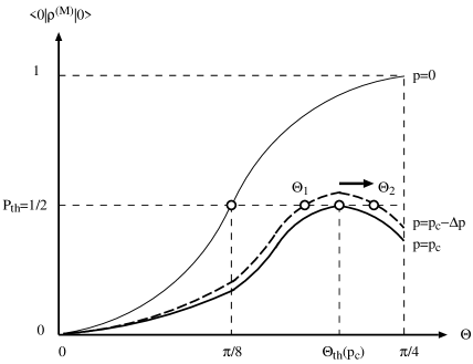
Figure 9: Variation of $\langle 0|\rho^{(M)}|0\rangle$ against $\Theta$ with $0\leq p\leq p_{\mbox{\scriptsize c}}$. The threshold of probability is set to $P_{\mbox{\scriptsize th}}=1/2$. White circles represent $\Theta_{\mbox{\scriptsize th}}(p)$ and $\tilde{\Theta}_{\mbox{\scriptsize th}}(x)$.

It can be explained as follows. Figure 9 illustrates a variation of $\langle 0|\rho^{(M)}|0\rangle$ against $\Theta$ for $0\leq p\leq p_{\mbox{\scriptsize c}}$. In the case of $p=0$ (no decoherence), we can obtain $\tilde{\Theta}_{\mbox{\scriptsize th}}(x=0)=\Theta_{\mbox{\scriptsize th}}(p=0)=\pi/8$ for $P_{\mbox{\scriptsize th}}=1/2$. (If $p=0$, we obtain $x=2Mnp=0$.) If we let $p$ get larger until $p=p_{\mbox{\scriptsize c}}$, $\Theta_{\mbox{\scriptsize th}}(p)$ increases gradually. Through this process, both $x$ and $\tilde{\Theta}_{\mbox{\scriptsize th}}(x)$ increase. When we reach at $p=p_{\mbox{\scriptsize c}}$, we obtain $\tilde{\Theta}_{\mbox{\scriptsize th}}(x)=\Theta_{\mbox{\scriptsize th}}(p_{\mbox{\scriptsize c}})<\pi/4$ for $x=2M_{\mbox{\scriptsize th}}(p)np_{\mbox{\scriptsize c}}<x_{\mbox{\scriptsize c}}$.

Although $p$ gets the allowed maximum value of $p_{\mbox{\scriptsize c}}$, we want to increase both $x$ and $\tilde{\Theta}_{\mbox{\scriptsize th}}(x)$ still more. To increase $x$, we take the following trick. We decrease $p$ by infinitesimal $\Delta p$, as shown in Figure 9. Then, $\langle 0|\rho^{(M)}|0\rangle$ takes $P_{\mbox{\scriptsize th}}=1/2$ at two points of $\Theta$, and we write them as $\Theta_{1}$ and $\Theta_{2}$ ($\Theta_{1}<\Theta_{2}$). At this time, we take the large one of them as $\tilde{\Theta}_{\mbox{\scriptsize th}}(x)$, so that $\tilde{\Theta}_{\mbox{\scriptsize th}}(x)=\Theta_{2}$.

Because $\langle 0|\rho^{(M)}|0\rangle$ takes the local minimum value at $\Theta_{\mbox{\scriptsize th}}(p_{\mbox{\scriptsize c}})$ for $p=p_{\mbox{\scriptsize c}}$, we can obtain

$$\left.\frac{\partial\langle 0|\rho^{(M)}|0\rangle}{\partial\Theta}\right|_{{\Theta=\Theta_{\mbox{\tiny th}}(p_{\mbox{\tiny c}})}\atop{p=p_{\mbox{\tiny c}}}}=\left.\frac{\partial\langle 0|\rho^{(M)}|0\rangle}{\partial\Theta_{\mbox{\scriptsize th}}(p)}\right|_{p=p_{\mbox{\tiny c}}}=\left.\frac{\partial\langle 0|\rho^{(M)}|0\rangle}{\partial p}\frac{\partial p}{\partial\Theta_{\mbox{\scriptsize th}}(p)}\right|_{p=p_{\mbox{\tiny c}}}=0,$$ (63)

$$\left.\frac{\partial\langle 0|\rho^{(M)}|0\rangle}{\partial p}\right|_{p=p_{\mbox{\tiny c}}}\neq 0,$$ (64)

and

$$\left.\frac{\partial p}{\partial\Theta_{\mbox{\scriptsize th}}(p)}\right|_{p=p_{\mbox{\tiny c}}}=0\quad\mbox{or}\quad\left.\frac{\partial\Theta_{\mbox{\scriptsize th}}(p)}{\partial p}\right|_{p=p_{\mbox{\tiny c}}}=-\infty.$$ (65)

Hence, the difference of $[\Theta_{2}-\Theta_{\mbox{\scriptsize th}}(p_{\mbox{\scriptsize c}})]$ can be quite large, and $\Theta_{2}(p_{\mbox{\scriptsize c}}-\Delta p)\geq\Theta_{\mbox{\scriptsize th}}(p_{\mbox{\scriptsize c}})p_{\mbox{\scriptsize c}}$ is possible. Therefore, we can make $\tilde{\Theta}_{\mbox{\scriptsize th}}(x)\geq\Theta_{\mbox{\scriptsize th}}(p_{\mbox{\scriptsize c}})$ and $x\geq 2M_{\mbox{\scriptsize th}}(p_{\mbox{\scriptsize c}})np_{\mbox{\scriptsize c}}$. (These considerations can be applied to $0<\forall P_{\mbox{\scriptsize th}}\leq 1$ as well.)

Figure 10: Variation of $x_{\mbox{\scriptsize c}}$ against $P_{\mbox{\scriptsize th}}$. A thick solid curve represents perturbation up to the fifth order. A thin dashed line shows its tangent at $P_{\mbox{\scriptsize th}}=1$ given by Eq. (67).

Then, we move on to the variation of $x_{\mbox{\scriptsize c}}$ against $P_{\mbox{\scriptsize th}}$, which is shown in Figure 10. We obtain it as follows. We calculate $\tilde{\Theta}_{\mbox{\scriptsize th}}(x)$ for given $P_{\mbox{\scriptsize th}}$ as varying $x$ from $0$. (We use the Newton’s method for obtaining a root of $\Theta$ for the equation of $P_{\mbox{\scriptsize rob}}(\Theta,x)=P_{\mbox{\scriptsize th}}$ with given $x$.) When $x$ gets a certain value, we cannot find a root for $\tilde{\Theta}_{\mbox{\scriptsize th}}(x)$, and we regard it as $x_{\mbox{\scriptsize c}}$. By repeating this calculation, we obtain the curve of Figure 10.

In these calculations, we notice $\tilde{\Theta}_{\mbox{\scriptsize th}}(x_{\mbox{\scriptsize c}};P_{\mbox{\scriptsize th}})\simeq\pi/4$ for the range of $x$ and $P_{\mbox{\scriptsize th}}$ where the perturbation theory is reliable ($0\leq x\leq 1.35$). It is caused by the approximately symmetric property of $F_{h}(\Theta)$ obtained in Section 7 and Appendix B as

$$F_{h}((\pi/4)+\Delta)\simeq F_{h}((\pi/4)-\Delta)\quad\quad\mbox{for $0<\Delta\ll(\pi/4)$ and $h=0,1,\cdots$}.$$ (66)

However, strictly speaking, $\tilde{\Theta}_{\mbox{\scriptsize th}}(x_{\mbox{\scriptsize c}};P_{\mbox{\scriptsize th}})$ cannot be a constant for $\forall x_{\mbox{\scriptsize c}}$ and $\forall P_{\mbox{\scriptsize th}}$.

Using Eq. (59), a tangent at $P_{\mbox{\scriptsize th}}=1$ is given by

$$x_{\mbox{\scriptsize c}}=c(1-P_{\mbox{\scriptsize th}}),\quad\quad c=-\frac{1}{C_{1}(\pi/4)}=\frac{8}{5},$$ (67)

because $\tilde{\Theta}_{\mbox{\scriptsize th}}(x_{\mbox{\scriptsize c}})=\pi/4$ and $x_{\mbox{\scriptsize c}}=0$ for $P_{\mbox{\scriptsize th}}=1$. It means that the algorithm is available for $2Mnp<(8/5)(1-P_{\mbox{\scriptsize th}})$ around $P_{\mbox{\scriptsize th}}\simeq 1$, and this relation approximately holds for a wide range of $P_{\mbox{\scriptsize th}}$. This result is similar to a work obtained by E. Bernstein and U. Vazirani [3]. We mention it in Section 9.1.

Figure 10 shows a transition about whether quantum computing is available or not for threshold probability $P_{\mbox{\scriptsize th}}$. Here, let us consider where is a classical searching on the phase diagram of Figure 10. We assume that we are looking for one item among unsorted $2^{n}$ items. If we examine $M$ items from them in a classical manner, we can find it with probability $P=M/2^{n}$. Now, let us regard $M$ as the number of the quantum operations iterated and $P$ as the threshold $P_{\mbox{\scriptsize th}}$ for the algorithm in classical regime. If we give $P_{\mbox{\scriptsize th}}>0$ (and it is not infinitesimal), the classical searching takes $M\simeq O(2^{n})$ and $x\gg x_{\mbox{\scriptsize c}}$. Hence, it is located far away upward in the non-available region of the quantum algorithm in Figure 10.

On the other hand, if we consider the neighbourhood of $P_{\mbox{\scriptsize th}}=0$, it becomes subtle. The classical searching can take small $M$, and it can approach to the available region of the quantum algorithm. Furthermore, in the limit of $P_{\mbox{\scriptsize th}}\rightarrow 0$, we can expect $M_{\mbox{\scriptsize th}}(p_{\mbox{\scriptsize c}})\rightarrow 0$ (but $n\rightarrow\infty$) for the quantum algorithm, so that behaviour of $x_{\mbox{\scriptsize c}}$ in the neighbourhood of $P_{\mbox{\scriptsize th}}=0$ might be singular.

From these discussions, we consider that a quantum to classical phase transition of the algorithm is described around $P_{\mbox{\scriptsize th}}\simeq 0$ in Figure 10. We cannot say anything about it by our approach, because $x_{\mbox{\scriptsize c}}$ for $P_{\mbox{\scriptsize th}}\simeq 0$ is outside the domain where the perturbation theory is reliable.

9 Discussions

In this section, we think about related work obtained by E. Bernstein and U. Vazirani, and how the phase error is caused. Then, we give other discussions about our results.

9.1 Accuracy of quantum gates

E. Bernstein and U. Vazirani consider accuracy of quantum gates for quantum computation [3][19]. Let us think about a quantum computer which is designed to apply $T$ unitary transformations, $U_{1},\cdots,U_{T}$, in succession ($T$ steps) to the initial state $|\phi_{0}\rangle$, as follows,

$$|\phi_{0}\rangle\stackrel{{\scriptstyle U_{1}}}{{\longrightarrow}}|\phi_{1}\rangle\stackrel{{\scriptstyle U_{2}}}{{\longrightarrow}}\cdots\stackrel{{\scriptstyle U_{T}}}{{\longrightarrow}}|\phi_{T}\rangle,$$ (68)

so that $|\phi_{t}\rangle=U_{t}|\phi_{t-1}\rangle$ and $\langle\phi_{t}|\phi_{t}\rangle=\langle\phi_{0}|\phi_{0}\rangle=1$ for $t=1,\cdots,T$. On the other hand, we assume that it actually applies $\tilde{U}_{t}$ which is slightly different from $U_{t}$ to the state because of incomplete accuracy,

$$|\phi_{0}\rangle\stackrel{{\scriptstyle\tilde{U}_{1}}}{{\longrightarrow}}|\tilde{\phi}_{1}\rangle\stackrel{{\scriptstyle\tilde{U}_{2}}}{{\longrightarrow}}\cdots\stackrel{{\scriptstyle\tilde{U}_{T}}}{{\longrightarrow}}|\tilde{\phi}_{T}\rangle,$$ (69)

so that $|\tilde{\phi}_{t}\rangle=\tilde{U}_{t}|\tilde{\phi}_{t-1}\rangle$, $|\tilde{\phi}_{0}\rangle=|\phi_{0}\rangle$, and $\langle\tilde{\phi}_{t}|\tilde{\phi}_{t}\rangle=1$ for $t=1,\cdots,T$. (We are considering errors of unitary transformations, and it does not cause dissipation to the quantum computer.)

Defining unnormalised states

$$|E_{t}\rangle=(\tilde{U}_{t}-U_{t})|\phi_{t-1}\rangle,$$ (70)

we obtain

$$|\tilde{\phi}_{1}\rangle = |\phi_{1}\rangle+|E_{1}\rangle,$$

$$|\tilde{\phi}_{2}\rangle = |\phi_{2}\rangle+|E_{2}\rangle+\tilde{U}_{2}|E_{1}\rangle,$$

$$\vdots$$

$$|\tilde{\phi}_{T}\rangle = |\phi_{T}\rangle+|E_{T}\rangle+\tilde{U}_{T}|E_{T-1}\rangle\cdots+\tilde{U}_{T}\tilde{U}_{T-1}\cdots\tilde{U}_{2}|E_{1}\rangle,$$ (71)

and

$$\langle\phi_{T}|\tilde{\phi}_{T}\rangle\geq 1-\sum_{t=1}^{T}\sqrt{\langle E_{t}|E_{t}\rangle}.$$ (72)

Here, we assume that the error of each step is bounded as

$$\sqrt{\langle E_{t}|E_{t}\rangle}\leq\epsilon\quad\quad\mbox{for $t=1,\cdots,T$}.$$ (73)

We obtain

$$|\langle\phi_{T}|\tilde{\phi}_{T}\rangle|^{2}\geq(1-T\epsilon)^{2}=1-2T\epsilon+O(\epsilon^{2}).$$ (74)

Hence, if the error of the unitary transformation at each step is bounded to $\epsilon$, the probability of detecting $|\phi_{T}\rangle$ that we want as the final state is at least $(1-2T\epsilon)$.

On the other hand, from Eq. (70), we obtain

$$\langle\phi_{t}|\tilde{U}_{T}|\phi_{t-1}\rangle=1+\langle\phi_{t}|E_{t}\rangle\geq 1-\epsilon,$$ (75)

and we can rewrite it with density operator as

$$\mbox{tr}(\rho\rho^{\prime})\geq 1-2\epsilon+O(\epsilon^{2}),$$ (76)

where $\rho=|\phi_{t}\rangle\langle\phi_{t}|$ and $\rho^{\prime}=\tilde{U}_{T}|\phi_{t}\rangle\langle\phi_{t}|\tilde{U}_{T}^{\dagger}$. In this paper, we consider the decoherence defined in Eq. (5). Although it is different from the error of unitary transformations in Eq. (69), we can obtain

$$\mbox{tr}(\rho\rho^{\prime})\geq 1-p,$$ (77)

and regard it as inaccuracy of operation for $\epsilon=p/2$ at each step.

If we require $|\langle\phi_{T}|\tilde{\phi}_{T}\rangle|^{2}>P_{\mbox{\scriptsize th}}$ for a threshold of the probability that the quantum computer gives a correct answer, we can obtain

$$1-P_{\mbox{\scriptsize th}}>1-|\langle\phi_{T}|\tilde{\phi}_{T}\rangle|^{2}\simeq 2T\epsilon,$$ (78)

as the first order estimation. Substituting $\epsilon=p/2$, and $T=2Mn$ which is the number of quantum gates during the whole process (the number of decoherences caused) into the above, we can obtain $2Mnp<1-P_{\mbox{\scriptsize th}}$. This is similar to the result obtained in Section 8, except for a factor.

9.2 How the phase error occurs

We give a mechanism which causes the phase error of Eq. (5) for an instance. We can think this error to be quite possible for proposed implementations of quantum computation [5]. Let us consider two spin-$1/2$ systems described as $3$-component normalised vectors of $\mbox{\boldmath$\sigma$}^{A}$ (qubit) and $\mbox{\boldmath$\sigma$}^{E}$ (environment), whose interaction is given by their inner product of $\kappa\mbox{\boldmath$\sigma$}^{A}\cdot\mbox{\boldmath$\sigma$}^{E}$.

If there is weak external magnetic field along $z$-direction $\mbox{\boldmath$B$}=(0,0,B_{z})$, both of them align themselves with $z$-direction, so that $\mbox{\boldmath$\sigma$}^{A}=(0,0,\pm 1)$ and $\mbox{\boldmath$\sigma$}^{E}=(0,0,\pm 1)$. Hence, we obtain an effective Hamiltonian of $\Delta H\simeq\kappa\sigma_{z}^{A}\sigma_{z}^{E}$, and a time-evolution operator

$$U_{\Delta}^{AE} = \exp(-i\frac{t}{\hbar}\Delta H)$$ (79)

$$= \bordermatrix{&\langle 00|&\langle 01|&\langle 10|&\langle 11|\cr|00\rangle&e^{-i\theta}&0&0&0\cr|01\rangle&0&e^{i\theta}&0&0\cr|10\rangle&0&0&e^{i\theta}&0\cr|11\rangle&0&0&0&e^{-i\theta}\cr},$$

on the logical basis $|ij\rangle=|i^{A}\rangle|i^{E}\rangle$ for $i,j\in\{0,1\}$, where $\theta=(\kappa/\hbar)t$.

We assume that the initial state of the systems $A$ and $E$ is given as $|\varphi^{A}\rangle|+^{E}\rangle$, where $|\varphi^{A}\rangle$ is an arbitrary state of $A$ and $|+^{E}\rangle=(1/\sqrt{2})(|0^{E}\rangle+i|1^{E}\rangle)$. It evolves as follows [20],

$$\rho^{A}=|\varphi^{A}\rangle\langle\varphi^{A}|\rightarrow\rho^{\prime A} = \mbox{tr}_{E}[U_{\Delta}^{AE}(|\varphi^{A}\rangle\langle\varphi^{A}|\otimes|+^{E}\rangle\langle+^{E}|)U_{\Delta}^{AE}{}^{\dagger}]$$ (80)

$$= \sum_{\mu\in\{+,-\}}M_{\mu}^{A}\rho^{A}M_{\mu}^{A}{}^{\dagger},$$

where

$$M_{\mu}^{A}=\langle\mu^{E}|U_{\Delta}^{AE}|+^{E}\rangle,$$ (81)

and

$$|\pm^{E}\rangle=\frac{1}{\sqrt{2}}(|0^{E}\rangle\pm i|1^{E}\rangle).$$ (82)

Here, we introduce a $2\times 2$ unitary transformation,

$$V=V^{\dagger}=\frac{1}{\sqrt{2}}\bordermatrix{&\langle 0|&\langle 1|\cr|0\rangle&1&1\cr|1\rangle&i&-i\cr},\quad\quad VV^{\dagger}=\mbox{\boldmath$I$},$$ (83)

and we obtain

$$|+^{E}\rangle=V^{E}|0^{E}\rangle,\quad\quad|-^{E}\rangle=V^{E}|1^{E}\rangle.$$ (84)

We can rewrite $M_{\mu}$ as

$$M_{+}^{A} = \langle 0^{E}|V^{E}{}^{\dagger}U_{\Delta}^{AE}V^{E}|0^{E}\rangle,$$

$$M_{-}^{A} = \langle 1^{E}|V^{E}{}^{\dagger}U_{\Delta}^{AE}V^{E}|0^{E}\rangle.$$ (85)

The matrix of Eq. (85) is given by

$$V^{E}{}^{\dagger}U_{\Delta}^{AE}V^{E} = \left[\begin{array}[]{c|c}V^{\dagger}&0\\ \hline\cr 0&V^{\dagger}\end{array}\right]\left[\begin{array}[]{c}\smash{\lower 8.61108pt\hbox{$U_{\Delta}^{AE}$}}\\ \\ \end{array}\right]\left[\begin{array}[]{c|c}V&0\\ \hline\cr 0&V\end{array}\right]$$ (92)

$$= \left[\begin{array}[]{c|c}R^{\dagger}&0\\ \hline\cr 0&R\end{array}\right],$$ (95)

on the logical basis, where

$$R=\left(\begin{array}[]{cc}\cos\theta&i\sin\theta\\ i\sin\theta&\cos\theta\end{array}\right).$$ (96)

Hence, we obtain

$$M_{+}=\cos\theta\mbox{\boldmath$I$}^{A}\quad\quad M_{-}=-i\sin\theta\sigma_{z}^{A}.$$ (97)

Therefore, the time evolution of the system $A$ is described as

$$\rho^{A}\rightarrow\rho^{\prime A}=\cos^{2}\theta\rho^{A}+\sin^{2}\theta\sigma_{z}\rho^{A}\sigma_{z},$$ (98)

and it is equivalent to Eq. (5).

If we assume that each qubit of the quantum computer interacts with an external spin-$1/2$ particle under the weak magnetic field every time interval, our model can give a reasonable description of its decoherence.

9.3 Other discussions

From Figure 10, we find $x_{\mbox{\scriptsize c}}=2\tilde{M}_{\mbox{\scriptsize th}}(x_{\mbox{\scriptsize c}})np\simeq O(1)$ for suitable threshold probability ($1/2\leq P_{\mbox{\scriptsize th}}\leq 1$, for example). It means that if the error ratio $p$ is smaller than an inverse of the number of quantum gates $(2Mn)^{-1}$, the algorithm is reliable. If this observation holds good for other quantum algorithms, it can serve a strong foundation to realize quantum computation. We cannot investigate a quantum to classical phase transition of the algorithm, because it is outside the reliable domain of our perturbation theory. For studying it precisely, we may need to construct an exact solvable model of a quantum system with decoherence.

Acknowledgements

We thank D. K. L. Oi and A. T. Costa, Jr. for helpful comments about Section 8. We also thank A. K. Ekert for encouragements.

Appendix A Formulas for deriving matrix elements of density operators

In this section, we collect some formulas that are used for deriving the matrix element of the density operator $T_{h}^{(M)}$.

A.1 Formulas of $(WR_{0})^{k}W|0\rangle$

We derive an explicit form of $(WR_{0})^{k}W|0\rangle$, where $|0\rangle$ is an $n$-qubit ($n\geq 2$) initial state of $|0\rangle\otimes\cdots\otimes|0\rangle$. Let us think an $n$-qubit state of

$$|\Psi\rangle=a_{0}|0\rangle+a_{1}\sum_{{x\neq 0}\atop{x\in\{0,1\}^{n}}}|x\rangle.$$ (99)

Using

$$W|x\rangle=\frac{1}{\sqrt{2^{n}}}\sum_{y\in\{0,1\}^{n}}(-1)^{x\cdot y}|y\rangle\quad\quad\mbox{for $\forall x\in\{0,1\}^{n}$},$$ (100)

where $x\cdot y$ represents an inner product of $n$-digit binary strings of $x,y\in\{0,1\}^{n}$, that is $x\cdot y=\sum_{i=1}^{n}x_{i}y_{i}$, we can derive

$$WR_{0}|\Psi\rangle = W(-a_{0}|0\rangle+a_{1}\sum_{x\neq 0}|x\rangle)$$ (101)

$$= \frac{1}{\sqrt{2^{n}}}[-a_{0}\sum_{y}|y\rangle+a_{1}\sum_{x\neq 0}\sum_{y}(-1)^{x\cdot y}|y\rangle]$$

$$= \frac{1}{\sqrt{2^{n}}}[(-a_{0}+(2^{n}-1)a_{1})|0\rangle-(a_{0}+a_{1})\sum_{y\neq 0}|y\rangle].$$

Then we introduce a parameter $\theta$ to simplify notations of states [14],

$$\sin\theta=\frac{1}{\sqrt{2^{n}}},\quad\quad\cos\theta=\sqrt{\frac{2^{n}-1}{2^{n}}}.$$ (102)

Using $\theta$, we obtain the following trigonometric formulas,

$$\frac{1}{\sqrt{2^{n}}}[\mp\sin\varphi+(2^{n}-1)\frac{\cos\varphi}{\sqrt{2^{n}-1}}] = \mp\sin\theta\sin\varphi+\cos\theta\cos\varphi$$ (103)

$$= \cos(\varphi\pm\theta),$$

$$\frac{1}{\sqrt{2^{n}}}[\mp\cos\varphi-(2^{n}-1)\frac{\sin\varphi}{\sqrt{2^{n}-1}}] = -\sin(\varphi\pm\theta),$$ (104)

$$\frac{1}{\sqrt{2^{n}}}(\pm\sin\varphi+\frac{\cos\varphi}{\sqrt{2^{n}-1}}) = \frac{1}{\sqrt{2^{n}-1}}(\pm\cos\theta\sin\varphi+\sin\theta\cos\varphi)$$ (105)

$$= \pm\frac{\sin(\varphi\pm\theta)}{\sqrt{2^{n}-1}},$$

$$\frac{1}{\sqrt{2^{n}}}(\pm\cos\varphi-\frac{\sin\varphi}{\sqrt{2^{n}-1}}) = \pm\frac{\cos(\varphi\pm\theta)}{\sqrt{2^{n}-1}}.$$ (106)

From these relations, we can obtain the following results,

$$W|0\rangle = \frac{1}{\sqrt{2^{n}}}\sum_{x}|x\rangle=\sin\theta|0\rangle+\frac{\cos\theta}{\sqrt{2^{n}-1}}\sum_{x\neq 0}|x\rangle,$$

$$(WR_{0})W|0\rangle = \cos 2\theta|0\rangle-\frac{\sin 2\theta}{\sqrt{2^{n}-1}}\sum_{x\neq 0}|x\rangle.$$ (107)

In general, we obtain

$$(WR_{0})^{2k}W|0\rangle = (-1)^{k}[\sin(2k+1)\theta|0\rangle+\frac{\cos(2k+1)\theta}{\sqrt{2^{n}-1}}\sum_{x\neq 0}|x\rangle]\quad\quad\mbox{for $k=0,1,\cdots$},$$ (108)

$$(WR_{0})^{2k+1}W|0\rangle = (-1)^{k}[\cos 2(k+1)\theta|0\rangle-\frac{\sin 2(k+1)\theta}{\sqrt{2^{n}-1}}\sum_{x\neq 0}|x\rangle]\quad\quad\mbox{for $k=0,1,\cdots$}.$$ (109)

A.2 Formulas of $(R_{0}W)^{k}|0\rangle$

From formulas obtained in Appendix A.1 we obtain

$$(R_{0}W)^{2k}|0\rangle = W(WR_{0})^{2k}W|0\rangle$$ (110)

$$= \frac{(-1)^{k}}{\sqrt{2^{n}}}[\sin(2k+1)\theta\sum_{x}|x\rangle+\frac{\cos(2k+1)\theta}{\sqrt{2^{n}-1}}(2^{n}|0\rangle-\sum_{x}|x\rangle)]$$

$$= \frac{(-1)^{k}}{\sqrt{2^{n}}}\{[\sin(2k+1)\theta+(2^{n}-1)\frac{\cos(2k+1)\theta}{\sqrt{2^{n}-1}}]|0\rangle$$

$$\quad\quad+[\sin(2k+1)\theta-\frac{\cos(2k+1)\theta}{\sqrt{2^{n}-1}}]\sum_{x\neq 0}|x\rangle\}$$

$$= (-1)^{k}[\cos 2k\theta|0\rangle+\frac{\sin 2k\theta}{\sqrt{2^{n}-1}}\sum_{x\neq 0}|x\rangle]\quad\quad\mbox{for $k=0,1,\cdots$},$$

$$(R_{0}W)^{2k+1}|0\rangle = (-1)^{k}[-\sin(2k+1)\theta|0\rangle+\frac{\cos(2k+1)\theta}{\sqrt{2^{n}-1}}\sum_{x\neq 0}|x\rangle]\quad\quad\mbox{for $k=0,1,\cdots$}.$$ (111)

A.3 Formulas for summation of trigonometric functions

When we calculate the matrix element of $\langle 0|T_{h}^{(M)}|0\rangle$, we often have to sum up trigonometric functions. In this paper, we use the following four formulas, which can be proved by the inductive method [21],

$$\sum_{l=0}^{n}(-1)^{l}\sin(2l+1)\theta = \frac{(-1)^{n}}{2}\frac{\sin 2(n+1)\theta}{\cos\theta}\quad\quad\mbox{for $n=0,1,\cdots$},$$ (112)

$$\sum_{l=0}^{n}(-1)^{l}\sin 2(l+1)\theta = \frac{\sin\theta}{2\cos\theta}+\frac{(-1)^{n}}{2\cos\theta}\sin(2n+3)\theta\quad\quad\mbox{for $n=0,1,\cdots$},$$ (113)

$$\sum_{l=0}^{n}(-1)^{l}\cos(2l+1)\theta = \frac{1+(-1)^{n}\cos 2(n+1)\theta}{2\cos\theta}\quad\quad\mbox{for $n=0,1,\cdots$},$$ (114)

$$\sum_{l=0}^{n}(-1)^{l}\cos 2(l+1)\theta = \frac{1}{2}+\frac{(-1)^{n}}{2\cos\theta}\cos(2n+3)\theta\quad\quad\mbox{for $n=0,1,\cdots$}.$$ (115)

A.4 Formulas of ${\cal G}^{(1)}(k,l)=\langle 0|(WR_{0})^{l}\sigma_{z}^{(i)}(WR_{0})^{k}W|0\rangle$

From Eqs. (108), (109), (110), and (111), we can derive the following formulas,

$${\cal G}^{(1)}(2k,2l) = \langle 0|(WR_{0})^{2l}\sigma_{z}^{(i)}(WR_{0})^{2k}W|0\rangle$$ (116)

$$= (-1)^{l+k}[\cos 2l\theta\langle 0|+\frac{\sin 2l\theta}{\sqrt{2^{n}-1}}\sum_{x\neq 0}\langle x|]$$

$$\times\sigma_{z}^{(i)}[\sin(2k+1)\theta|0\rangle+\frac{\cos(2k+1)\theta}{\sqrt{2^{n}-1}}\sum_{y\neq 0}|y\rangle]$$

$$= (-1)^{l+k}[\cos 2l\theta\sin(2k+1)\theta-\frac{1}{2^{n}-1}\sin 2l\theta\cos(2k+1)\theta]$$

$$\quad\quad\mbox{for $k=0,1,\cdots$, $l=1,2,\cdots$},$$

$${\cal G}^{(1)}(2k,2l+1) = \langle 0|(WR_{0})^{2l+1}\sigma_{z}^{(i)}(WR_{0})^{2k}W|0\rangle$$ (117)

$$= (-1)^{l+k}[-\sin(2l+1)\theta\sin(2k+1)\theta-\frac{1}{2^{n}-1}\cos(2l+1)\theta\cos(2k+1)\theta]$$

$$\quad\quad\mbox{for $k=0,1,\cdots$, $l=0,1,\cdots$},$$

$${\cal G}^{(1)}(2k+1,2l) = \langle 0|(WR_{0})^{2l}\sigma_{z}^{(i)}(WR_{0})^{2k+1}W|0\rangle$$ (118)

$$= (-1)^{l+k}[\cos 2l\theta\cos 2(k+1)\theta+\frac{1}{2^{n}-1}\sin 2l\theta\sin 2(k+1)\theta]$$

$$\quad\quad\mbox{for $k=0,1,\cdots$, $l=1,2,\cdots$},$$

$${\cal G}^{(1)}(2k+1,2l+1) = \langle 0|(WR_{0})^{2l+1}\sigma_{z}^{(i)}(WR_{0})^{2k+1}W|0\rangle$$ (119)

$$= (-1)^{l+k}[-\sin(2l+1)\theta\cos 2(k+1)\theta+\frac{1}{2^{n}-1}\cos(2l+1)\theta\sin 2(k+1)\theta]$$

$$\quad\quad\mbox{for $k=0,1,\cdots$, $l=0,1,\cdots$},$$

A.5 Formulas of $\langle 0|(WR_{0})^{k}\sigma_{z}^{(i)}|\eta_{j}\rangle$ and $(1/\sqrt{2})\langle 0|(WR_{0})^{k}\sigma_{z}^{(i)}(|0\rangle-|\overline{j}\rangle)$

From Eqs. (23), (26) in Section 5, and Eqs. (110), (111) in Appendix A.2, we can derive the following formulas,

$$\langle 0|(WR_{0})^{2k}\sigma_{z}^{(i)}|\eta_{j}\rangle = (-1)^{k}[\cos 2k\theta\langle 0|+\frac{\sin 2k\theta}{\sqrt{2^{n}-1}}\sum_{x\neq 0}\langle x|]\sigma_{z}^{(i)}\frac{1}{\sqrt{2^{n-1}}}\sum_{y_{j}=1}|y\rangle$$ (120)

$$= (-1)^{k}\frac{\sin 2k\theta}{\sqrt{2^{n}-1}\sqrt{2^{n-1}}}\delta_{ij}(-1)2^{n-1}$$

$$= -(-1)^{k}\sqrt{\frac{2^{n-1}}{2^{n}-1}}\sin 2k\theta\delta_{ij}$$

$$= -\frac{(-1)^{k}}{\sqrt{2}}\frac{\sin 2k\theta}{\cos\theta}\delta_{ij},$$

$$\langle 0|(WR_{0})^{2k+1}\sigma_{z}^{(i)}|\eta_{j}\rangle = -\frac{(-1)^{k}}{\sqrt{2}}\frac{\cos(2k+1)\theta}{\cos\theta}\delta_{ij},$$ (121)

$$\frac{1}{\sqrt{2}}\langle 0|(WR_{0})^{2k}\sigma_{z}^{(i)}(|0\rangle-|\overline{j}\rangle) = \frac{1}{\sqrt{2}}(-1)^{k}[\cos 2k\theta\langle 0|+\frac{\sin 2k\theta}{\sqrt{2^{n}-1}}\sum_{x\neq 0}\langle x|]\sigma_{z}^{(i)}(|0\rangle-|\overline{j}\rangle)$$ (122)

$$= \frac{(-1)^{k}}{\sqrt{2}}[\cos 2k\theta-(-1)^{\delta_{ij}}\frac{\sin 2k\theta}{\sqrt{2^{n}-1}}],$$

$$\frac{1}{\sqrt{2}}\langle 0|(WR_{0})^{2k+1}\sigma_{z}^{(i)}(|0\rangle-|\overline{j}\rangle) = -\frac{(-1)^{k}}{\sqrt{2}}[\sin(2k+1)\theta+(-1)^{\delta_{ij}}\frac{\cos(2k+1)\theta}{\sqrt{2^{n}-1}}].$$ (123)

A.6 Derivation of the asymptotic forms of matrix elements

In this section, we derive the asymptotic forms of matrix elements, Eqs. (54) and (56) introduced in Section 7.

Comparing Eqs. (45) and (51), we notice that contributions of $\langle 0|T_{h}^{(M)}|0\rangle/(Mn)^{h}$ under $n\rightarrow\infty$ comes from only terms in which $\sigma_{z}$ errors occur at different steps and different qubits. The reason is as follows. The term of

$$|\langle 0|[\mbox{product of $(WR_{0})$s and $\sigma_{z}$s}]|0\rangle|^{2}$$ (124)

never exceeds unity, and the number of terms where $\sigma_{z}$ errors occur at the same step or the same qubit in $\langle 0|T_{h}^{(M)}|0\rangle$ is at most $O((2M)^{h}n^{h-1})$. Because we divide $\langle 0|T_{h}^{(M)}|0\rangle$ by $(Mn)^{h}$, they are eliminated under $n\rightarrow\infty$, as far as $h$ is finite.

Figure 11: Diagram of $h$ errors, ${\cal G}^{(h)}(l_{0},l_{1},\cdots,l_{h})$.

An asymptotic form of the matrix element with $h$ errors at different steps and qubits, as shown in Figure 11, are given by

$$\lim_{n\rightarrow\infty}{\cal G}^{(h)}(l_{0},l_{1},\cdots,l_{h})$$ (125)

$$\equiv \lim_{n\rightarrow\infty}\langle 0|(WR_{0})^{l_{h}}\sigma_{z}^{(i_{h})}\cdots(WR_{0})^{l_{1}}\sigma_{z}^{(i_{1})}(WR_{0})^{l_{0}}W|0\rangle$$

$$= (-1)^{\sum_{s=0}^{h}\lfloor l_{s}/2\rfloor+\sum_{s=1}^{h}\alpha_{s}}{\sin\brace{\cos}}_{\alpha_{0}}((l_{0}+1)\theta){\cos\brace{\sin}}_{\alpha_{1}}(l_{1}\theta)\cdots{\cos\brace{\sin}}_{\alpha_{h}}(l_{h}\theta)$$

$$\quad\quad\mbox{for $h=1,2,\cdots$},$$

where $l_{0}=0,1,\cdots$, $l_{s}=1,2,\cdots$ for $s=1,\cdots,h$, $\{i_{s}:1\leq i_{s}\leq n$ for $s=1,\cdots,h\}$ are different from each other, $\lfloor x\rfloor$ represents the largest integer that is less than or equal to $x$,

$$\alpha_{s}=l_{s}(\mbox{mod $2$})\in\{0,1\}\quad\quad\mbox{for $s=0,\cdots,h$},$$ (126)

and

$${f\brace{g}}_{\alpha}(x)\equiv\left\{\begin{array}[]{ll}f(x)&\mbox{for $\alpha=0$}\\ g(x)&\mbox{for $\alpha=1$}\end{array}\right..$$ (127)

We show that this holds for $h=1$ in Appendix A.4. We prove Eq. (125) for arbitrary $h$ by the inductive method. Let us assume Eq. (125) is satisfied for $h$. We examine whether it is satisfied for $(h+1)$ or not.

First, we assume $l_{0}=2m$ and $l_{1}=2\tilde{m}$ (both of them are even). Using Eq. (30), we obtain

$${\cal G}^{(h+1)}(2m,2\tilde{m},l_{2},\cdots,l_{h+1})$$ (128)

$$= \langle 0|(WR_{0})^{l_{h+1}}\sigma_{z}^{(i_{h+1})}\cdots(WR_{0})^{l_{2}}\sigma_{z}^{(i_{2})}\biggl{[}(WR_{0})^{2\tilde{m}}\sigma_{z}^{(i_{1})}(WR_{0})^{2m}W|0\rangle\biggr{]}$$

$$\sim {\cal G}^{(h)}(2(m+\tilde{m}),l_{2},\cdots,l_{h+1})$$

$$-\sqrt{2}(-1)^{m}\cos(2m+1)\theta[-\sqrt{2}\sum_{k=0}^{\tilde{m}-1}{\cal G}^{(h)}(2k,l_{2},\cdots,l_{h+1})$$

$$+\langle 0|(WR_{0})^{l_{h+1}}\sigma_{z}^{(i_{h+1})}\cdots(WR_{0})^{l_{2}}\sigma_{z}^{(i_{2})}|\eta_{i_{1}}\rangle]$$

$$\quad\quad\mbox{for $m=0,1,\cdots$, $\tilde{m}=1,2,\cdots$, as $n\rightarrow\infty$},$$

where we use $\lim_{n\rightarrow\infty}\cos\theta=1$. (We eliminate one $\sigma_{z}$ operator from the above equation. This technique is used in Sections 5 and 6.) From now on, we use a symbol of ‘$\sim$’ as an asymptotic equal sign under $n\rightarrow\infty$ for a while. On the other hand,

$$\langle 0|(WR_{0})^{l_{h+1}}\sigma_{z}^{(i_{h+1})}\cdots(WR_{0})^{l_{2}}\sigma_{z}^{(i_{2})}|\eta_{i_{1}}\rangle=0,$$ (129)

which is proved in Appendix A.7. Substituting Eq. (125) for $h$ and Eq. (129) into Eq. (128), and using Eq. (112), we obtain

$${\cal G}^{(h+1)}(2m,2\tilde{m},l_{2},\cdots,l_{h+1})$$ (130)

$$\sim (-1)^{m+\tilde{m}}\sin(2m+2\tilde{m}+1)\theta{\cal F}(l_{2},\cdots,l_{h+1})$$

$$+2(-1)^{m}\cos(2m+1)\theta\sum_{k=0}^{\tilde{m}-1}(-1)^{k}\sin(2k+1)\theta{\cal F}(l_{2},\cdots,l_{h+1})$$

$$= (-1)^{m}[(-1)^{\tilde{m}}\sin(2m+2\tilde{m}+1)\theta+2\cos(2m+1)\theta\frac{(-1)^{\tilde{m}-1}}{2}\frac{\sin 2\tilde{m}\theta}{\cos\theta}]{\cal F}(l_{2},\cdots,l_{h+1})$$

$$\sim (-1)^{m+\tilde{m}}\sin(2\tilde{m}+1)\theta\cos 2\tilde{m}\theta{\cal F}(l_{2},\cdots,l_{h+1})\quad\quad\mbox{as $n\rightarrow\infty$},$$

where

$${\cal F}(l_{2},\cdots,l_{h+1})=(-1)^{\sum_{s=2}^{h+1}\lfloor l_{s}/2\rfloor+\sum_{s=2}^{h+1}\alpha_{s}}{\cos\brace{\sin}}_{\alpha_{2}}(l_{2}\theta)\cdots{\cos\brace{\sin}}_{\alpha_{h+1}}(l_{h+1}\theta).$$ (131)

This means Eq. (125) is satisfied for $(h+1)$ with $(l_{0},l_{1})=(2m,2\tilde{m})$.

Next, we assume $l_{0}=2m$ and $l_{1}=2\tilde{m}+1$ (even and odd). From Eqs. (22) and (29), we obtain

$${\cal G}^{(h+1)}(2m,2\tilde{m}+1,l_{2},\cdots,l_{h+1})$$ (132)

$$= \langle 0|(WR_{0})^{l_{h+1}}\sigma_{z}^{(i_{h+1})}\cdots(WR_{0})^{l_{2}}\sigma_{z}^{(i_{2})}\biggl{[}(WR_{0})^{2\tilde{m}+1}\sigma_{z}^{(i_{1})}(WR_{0})^{2m}W|0\rangle\biggr{]}$$

$$\sim {\cal G}^{(h)}((2m+2\tilde{m})+1,l_{2},\cdots,l_{h+1})$$

$$-\sqrt{2}(-1)^{m}\cos(2m+1)\theta[-\sqrt{2}\sum_{k=0}^{\tilde{m}-1}{\cal G}^{(h)}(2k+1,l_{2},\cdots,l_{h+1})$$

$$+\frac{1}{\sqrt{2}}\langle 0|(WR_{0})^{l_{h+1}}\sigma_{z}^{(i_{h+1})}\cdots(WR_{0})^{l_{2}}\sigma_{z}^{(i_{2})}(|0\rangle-|\overline{i_{1}}\rangle)]$$

$$\quad\quad\mbox{for $m=0,1,\cdots$, $\tilde{m}=1,2,\cdots$, as $n\rightarrow\infty$}.$$

(We eliminate one $\sigma_{z}$ operator from the above expression as well as Eq. (128).) On the other hand,

$$\langle 0|(WR_{0})^{l_{h+1}}\sigma_{z}^{(i_{h+1})}\cdots(WR_{0})^{l_{2}}\sigma_{z}^{(i_{2})}(|0\rangle-|\overline{i_{1}}\rangle)\sim{\cal F}(l_{2},\cdots,l_{h+1})\quad\quad\mbox{as $n\rightarrow\infty$},$$ (133)

which is proved in Appendix A.8. Hence, substituting Eq. (125) for $h$ and Eq. (133) into Eq. (132), and using Eq.(115), we obtain

$${\cal G}^{(h+1)}(2m,2\tilde{m}+1,l_{2},\cdots,l_{h+1})$$ (134)

$$\sim \{(-1)^{m+\tilde{m}}\cos 2(m+\tilde{m}+1)\theta$$

$$+2(-1)^{m}\cos(2m+1)\theta[\sum_{k=0}^{\tilde{m}-1}(-1)^{k}\cos 2(k+1)\theta-\frac{1}{2}]\}{\cal F}(l_{2},\cdots,l_{h+1})$$

$$= (-1)^{m}\{(-1)^{\tilde{m}}\cos 2(m+\tilde{m}+1)\theta$$

$$+2\cos(2m+1)\theta[\frac{1}{2}+\frac{(-1)^{\tilde{m}-1}}{2\cos\theta}\cos(2\tilde{m}+1)\theta-\frac{1}{2}]\}{\cal F}(l_{2},\cdots,l_{h+1})$$

$$\sim (-1)^{m+\tilde{m}+1}\sin(2m+1)\theta\sin(2\tilde{m}+1)\theta{\cal F}(l_{2},\cdots,l_{h+1})\quad\quad\mbox{as $n\rightarrow\infty$}.$$

This means Eq. (125) holds for $(h+1)$ with $(l_{0},l_{1})=(2m,2\tilde{m}+1)$.

In the case of $(l_{0},l_{1})=(2m+1,2\tilde{m})$, and $(2m+1,2\tilde{m}+1)$, we can show Eq. (125) is satisfied for $(h+1)$ in similar ways. Therefore, we obtain Eq. (125) for $h=1,2,\cdots$ by induction. We pay attention that it does not depend on $i_{1},\cdots,i_{h}$.

To obtain an asymptotic form of $\langle 0|T_{h}^{(M)}|0\rangle/(Mn)^{h}$, we take intervals of Figure 11 as $l_{0},\cdots,l_{h-1},2M-\sum_{s=1}^{h-1}l_{s}$, multiply a factor $n!/(n-h)!$ to the terms for permutation of $\sigma_{z}$ errors, and sum up them by $l_{0},\cdots,l_{h-1}$,

$$\lim_{n\rightarrow\infty}\frac{\langle 0|T_{h}^{(M)}|0\rangle}{(Mn)^{h}} = \lim_{n\rightarrow\infty}\frac{1}{(Mn)^{h}}\sum_{l_{0}=0}^{M-h}\sum_{l_{1}=1}^{M-h-l_{0}}\cdots\sum_{l_{h-1}=1}^{M-h-(l_{0}+\cdots+l_{h-2})}$$ (135)

$$\times\frac{n!}{(n-h)!}|{\cal G}^{(h)}(l_{0},\cdots,l_{h+1},2M-\sum_{s=1}^{h-1}l_{s})|^{2}.$$

Then, substituting Eq. (125), $\Theta=\lim_{n\rightarrow\infty}M\theta$, $\phi_{s+1}=l_{s}\theta$ for $s=0,\cdots,h-1$,

$$\lim_{n\rightarrow\infty}\sum_{l_{0}=0}^{M-h}\theta=\int_{0}^{\Theta}d\phi_{1},$$ (136)

and

$$\lim_{n\rightarrow\infty}\sum_{l_{s}=1}^{M-h-\sum_{t=0}^{s-1}l_{t}}\theta=\int_{0}^{\Theta-\sum_{t=1}^{s}\phi_{t}}d\phi_{s+1}\quad\quad\mbox{for $s=1,\cdots,h-1$},$$ (137)

into Eq. (135), we obtain Eqs. (54) and (56).

A.7 Formulas of $\langle 0|(WR_{0})^{l_{h}}\sigma_{z}^{(i_{h})}\cdots(WR_{0})^{l_{1}}\sigma_{z}^{(i_{1})}|\eta_{i_{0}}\rangle$

In this section, we show

$$\langle 0|(WR_{0})^{l_{h}}\sigma_{z}^{(i_{h})}\cdots(WR_{0})^{l_{1}}\sigma_{z}^{(i_{1})}|\eta_{i_{0}}\rangle=0,$$ (138)

for $h=1,2,\cdots$, where $l_{s}=1,2,\cdots$ for $s=1,\cdots,h$, and $\{i_{s}:1\leq i_{s}\leq n\quad\mbox{for $s=0,1,\cdots,h$}\}$ are different from each other. For $h=1$, it is proved in Appendix A.5.

To prove Eq. (138) for arbitrary $h$, we need to show

$$\langle 0|(WR_{0})^{l_{h}}\sigma_{z}^{(i_{h})}\cdots(WR_{0})^{l_{1}}\sigma_{z}^{(i_{1})}|\eta_{j_{1},\cdots,j_{s}}\rangle=0$$ (139)

$$\quad\quad\mbox{for $\{i_{1},\cdots,i_{h},j_{1},\cdots,j_{s}\}$ that are different from each other},$$

$$\langle 0|(WR_{0})^{l_{h}}\sigma_{z}^{(i_{h})}\cdots(WR_{0})^{l_{1}}\sigma_{z}^{(i_{1})}(|\overline{j_{0},j_{1},\cdots,j_{s}}\rangle-|\overline{j_{1},\cdots,j_{s}}\rangle)=0$$ (140)

$$\quad\quad\mbox{for $\{i_{1},\cdots,i_{h},j_{0},j_{1},\cdots,j_{s}\}$ that are different from each other},$$

where $1\leq j_{0}\leq n$, $\cdots$, $1\leq j_{s}\leq n$,

$$|\eta_{j_{1},\cdots,j_{s}}\rangle=\frac{1}{\sqrt{2^{n-s}}}\sum_{x_{j_{1}}=\cdots=x_{j_{s}}=1}|x\rangle,$$ (141)

and

$$|\overline{j_{0},j_{1},\cdots,j_{s}}\rangle=|0\cdots 0\begin{array}[t]{c}1\\ \uparrow\\ j_{0}\end{array}0\cdots 0\begin{array}[t]{c}1\\ \uparrow\\ j_{1}\end{array}0\cdots 0\begin{array}[t]{c}1\\ \uparrow\\ j_{s}\end{array}0\cdots 0\rangle.$$ (142)

From similar calculations in Appendix A.5, we can show Eqs. (139) and (140) are satisfied for $h=1$. We prove them for arbitrary $h$ by the inductive method.

Let us derive an explicit form of

$$(WR_{0})^{l}\sigma_{z}^{(i)}|\eta_{j_{1},\cdots,j_{s}}\rangle\quad\quad\mbox{for $l=1,2,\cdots$},$$ (143)

which appears in Eq. (139). At first, we consider the case of $s=1$. We can obtain

$$\sigma_{z}^{(i)}|\eta_{j}\rangle = \frac{1}{\sqrt{2^{n-1}}}(\sum_{{y_{j}=1}\atop{y_{i}=0}}-\sum_{{y_{j}=1}\atop{y_{i}=1}})|y\rangle$$ (144)

$$= |\eta_{j}\rangle-\sqrt{2}|\eta_{j,i}\rangle\quad\quad\mbox{for $i\neq j$}.$$

Then, we derive an explicit form of $(WR_{0})^{l}|\eta_{i,j}\rangle$. In the case of $l=1$, we obtain

$$WR_{0}|\eta_{i,j}\rangle=\frac{1}{2}(|0\rangle-|\overline{i}\rangle-|\overline{j}\rangle+|\overline{i,j}\rangle).$$ (145)

For $l=2$, we obtain

$$(WR_{0})^{2}|\eta_{i,j}\rangle = -\frac{1}{2}W(|0\rangle+|\overline{i}\rangle+|\overline{j}\rangle-|\overline{i,j}\rangle)$$ (146)

$$= -\frac{1}{2\sqrt{2^{n}}}(2\sum_{x}|x\rangle-4\sum_{x_{i}=x_{j}=1}|x\rangle)$$

$$= -W|0\rangle+|\eta_{i,j}\rangle.$$

Hence, we obtain

$$(WR_{0})^{2l}|\eta_{i,j}\rangle = -\sum_{k=0}^{l-1}(WR_{0})^{2k}W|0\rangle+|\eta_{i,j}\rangle\quad\quad\mbox{for $l=0,1,\cdots$},$$ (147)

$$(WR_{0})^{2l+1}|\eta_{i,j}\rangle = -\sum_{k=0}^{l-1}(WR_{0})^{2k+1}W|0\rangle+\frac{1}{2}(|0\rangle-|\overline{i}\rangle-|\overline{j}\rangle+|\overline{i,j}\rangle)\quad\quad\mbox{for $l=0,1,\cdots$}.$$ (148)

From Eqs. (28), (144), and (147), we obtain

$$(WR_{0})^{2l}\sigma_{z}^{(i)}|\eta_{j}\rangle = (WR_{0})^{2l}|\eta_{j}\rangle-\sqrt{2}(WR_{0})^{2l}|\eta_{j,i}\rangle$$ (149)

$$= -\sqrt{2}\sum_{k=0}^{l-1}(WR_{0})^{2k}W|0\rangle+|\eta_{j}\rangle+\sqrt{2}\sum_{k=0}^{l-1}(WR_{0})^{2k}W|0\rangle-\sqrt{2}|\eta_{j,i}\rangle$$

$$= |\eta_{j}\rangle-\sqrt{2}|\eta_{j,i}\rangle$$

$$= \sigma_{z}^{(i)}|\eta_{j}\rangle\quad\quad\mbox{for $l=0,1,\cdots$}.$$

Furthermore, using Eqs. (29) and (148), we obtain

$$(WR_{0})^{2l+1}\sigma_{z}^{(i)}|\eta_{j}\rangle = WR_{0}\sigma_{z}^{(i)}|\eta_{j}\rangle$$ (150)

$$= WR_{0}(|\eta_{j}\rangle-\sqrt{2}|\eta_{j,i}\rangle)$$

$$= \frac{1}{\sqrt{2}}(|\overline{i}\rangle-|\overline{j,i}\rangle)\quad\quad\mbox{for $l=0,1,\cdots$}.$$

In general, from similar calculations above, we can obtain

$$(WR_{0})^{2l}\sigma_{z}^{(i)}|\eta_{j_{1},\cdots,j_{s}}\rangle=|\eta_{j_{1},\cdots,j_{s}}\rangle-\sqrt{2}|\eta_{j_{1},\cdots,j_{s},i}\rangle\quad\quad\mbox{for $l=0,1,\cdots$},$$ (151)

$$(WR_{0})^{2l+1}\sigma_{z}^{(i)}|\eta_{j_{1},\cdots,j_{s}}\rangle$$ (153)

$$= \frac{1}{\sqrt{2^{s}}}\sum_{\alpha\in\{0,1\}^{s}}(-1)^{\alpha_{1}+\cdots+\alpha_{s}}|\overline{i,\alpha_{1}j_{1},\cdots,\alpha_{s}j_{s}}\rangle$$

$$= \frac{1}{\sqrt{2^{s}}}\sum_{(\alpha_{2},\cdots,\alpha_{s})\in\{0,1\}^{s-1}}(-1)^{\alpha_{2}+\cdots+\alpha_{s}}(|\overline{i,0,\alpha_{2}j_{2},\cdots,\alpha_{s}j_{s}}\rangle-|\overline{i,j_{1},\alpha_{2}j_{2},\cdots,\alpha_{s}j_{s}}\rangle)$$

$$\quad\quad\mbox{for $l=0,1,\cdots$},$$

where

$$|\overline{i,\alpha_{1}j_{1},\cdots,\alpha_{s}j_{s}}\rangle=|0\cdots 0\begin{array}[t]{c}1\\ \uparrow\\ i\end{array}0\cdots 0\begin{array}[t]{c}\alpha_{1}\\ \uparrow\\ j_{1}\end{array}0\cdots 0\begin{array}[t]{c}\alpha_{s}\\ \uparrow\\ j_{s}\end{array}0\cdots 0\rangle.$$ (154)

Here, we notice that, if we relabel indexes, the right side of Eq. (153) is written as a sum of $(|\overline{j_{0},j_{1},\cdots,j_{r}}\rangle-|\overline{j_{1},\cdots,j_{r}}\rangle)$, which appears in Eq. (140).

Then, we derive an explicit form of

$$(WR_{0})^{l}\sigma_{z}^{(i)}(|\overline{j_{0},j_{1},\cdots,j_{s}}\rangle-|\overline{j_{1},\cdots,j_{s}}\rangle)\quad\quad\mbox{for $l=1,2,\cdots$},$$ (155)

included by Eq. (140). Here, we can assume $j_{t}=t$ for $t=1,\cdots,s$, and $s<i\leq n$, without losing generality. Because $\{i,j_{0},\cdots,j_{s}\}$ are different from each other, $\sigma_{z}^{(i)}$ does not have an effect on the state. Hence, we obtain

$$(WR_{0})^{l}\sigma_{z}^{(i)}(|\underbrace{1,\cdots,1}_{s+1},\underbrace{0,\cdots,0}_{n-s-1}\rangle-|0,\underbrace{1,\cdots,1}_{s},\underbrace{0,\cdots,0}_{n-s-1}\rangle)$$ (158)

$$= \left\{\begin{array}[]{ll}{\displaystyle|\underbrace{1,\cdots,1}_{s+1},\underbrace{0,\cdots,0}_{n-s-1}\rangle-|0,\underbrace{1,\cdots,1}_{s},\underbrace{0,\cdots,0}_{n-s-1}\rangle}&\mbox{for $l=0,2,\cdots$ (even)}\\ {\displaystyle\frac{1}{\sqrt{2^{n-2}}}\sum_{x\in\{0,1\}^{n-1}}(-1)^{1+x_{1}+\cdots+x_{s}}|1,x_{1},\cdots,x_{n-1}\rangle}&\mbox{for $l=1,3,\cdots$ (odd)}\end{array}\right..$$

From this result, we find that Eq. (155) is described as a sum of $(|\overline{j_{0},j_{1},\cdots,j_{s}}\rangle-|\overline{j_{1},\cdots,j_{s}}\rangle)$, which appears in Eq. (140).

Here, we assume Eqs. (139) and (140) hold for $h$. From Eqs. (151), (153), and (158), we can resolve Eqs. (139) and (140) for $(h+1)$ to terms that contain $h$ errors of $\sigma_{z}$, so that we can prove them to be true for $(h+1)$. Hence, they are proved for any $h$ by the inductive method. Therefore, we obtain Eq. (138) for arbitrary $h$.

A.8 Formulas of $\langle 0|(WR_{0})^{l_{h}}\sigma_{z}^{(i_{h})}\cdots(WR_{0})^{l_{1}}\sigma_{z}^{(i_{1})}(|0\rangle-|\overline{i_{0}}\rangle)$

In this section, we show

$$\langle 0|(WR_{0})^{l_{h}}\sigma_{z}^{(i_{h})}\cdots(WR_{0})^{l_{1}}\sigma_{z}^{(i_{1})}(|0\rangle-|\overline{i_{0}}\rangle)\sim{\cal F}(l_{1},\cdots,l_{h})\quad\quad\mbox{as $n\rightarrow\infty$},$$ (159)

for $h=1,2,\cdots$, where $l_{s}=1,2,\cdots$ for $s=1,\cdots,h$, $\{i_{s}:1\leq i_{s}\leq n\quad\mbox{for $s=0,1,\cdots,h$}\}$ are different from each other, and the function ${\cal F}(l_{1},\cdots,l_{h})$ is defined in Eq. (131) of Appendix A.6. Eq. (159) is used for the inductive method in Appendix A.6. It is shown for $h=1$ in Appendix A.5. We prove it for any $h$ by the inductive method.

We assume Eq. (159) is satisfied for $(h-1)$. Let us consider the following equation,

$$(WR_{0})^{l}\sigma_{z}^{(i)}(|0\rangle-|\overline{j}\rangle) = -(WR_{0})^{l-1}W(|0\rangle+|\overline{j}\rangle)$$ (160)

$$= -(WR_{0})^{l-1}(2W|0\rangle-\sqrt{2}|\eta_{j}\rangle)\quad\quad\mbox{for $l=1,2,\cdots$ and $i\neq j$}.$$

Here, we assume $l=2m+1$ (odd). From Eq. (28), we obtain

$$(WR_{0})^{2m+1}\sigma_{z}^{(i)}(|0\rangle-|\overline{j}\rangle) = -2(WR_{0})^{2m}W|0\rangle+\sqrt{2}(WR_{0})^{2m}|\eta_{j}\rangle$$ (161)

$$= -2(WR_{0})^{2m}W|0\rangle-2\sum_{k=0}^{m-1}(WR_{0})^{2k}W|0\rangle+\sqrt{2}|\eta_{j}\rangle$$

$$= -2\sum_{k=0}^{m}(WR_{0})^{2k}W|0\rangle+\sqrt{2}|\eta_{j}\rangle.$$

Using Eq. (138), we obtain

$$\langle 0|(WR_{0})^{l_{h}}\sigma_{z}^{(i_{h})}\cdots(WR_{0})^{l_{2}}\sigma_{z}^{(i_{2})}(WR_{0})^{2m+1}\sigma_{z}^{(i_{1})}(|0\rangle-|\overline{i_{0}}\rangle)=-2\sum_{k=0}^{m}{\cal G}^{(h-1)}(2k,l_{2},\cdots,l_{h}).$$ (162)

Then, we consider the following fact. We use Eq. (159) for obtaining the asymptotic form of Eq. (125) by induction in Appendix A.6. Hence, we can assume that Eq. (125) is true for $(h-1)$. Therefore, we can require Eq. (162) as

$$\langle 0|(WR_{0})^{l_{h}}\sigma_{z}^{(i_{h})}\cdots(WR_{0})^{l_{2}}\sigma_{z}^{(i_{2})}(WR_{0})^{2m+1}\sigma_{z}^{(i_{1})}(|0\rangle-|\overline{i_{0}}\rangle)$$ (163)

$$\sim -2\sum_{k=0}^{m}(-1)^{k}\sin(2k+1)\theta{\cal F}(l_{2},\cdots,l_{h})$$

$$\sim (-1)^{m+1}\sin 2(m+1)\theta{\cal F}(l_{2},\cdots,l_{h})$$

$$\sim (-1)^{m+1}\sin(2m+1)\theta{\cal F}(l_{2},\cdots,l_{h})$$

$$= {\cal F}(2m+1,l_{2},\cdots,l_{h})\quad\quad\mbox{as $n\rightarrow\infty$},$$

where we use Eq. (112) and $\sin 2(m+1)\theta\sim\sin(2m+1)\theta$.

Hence, Eq. (159) is satisfied for $h$ in the case that $l$ is odd. For $l=2m$ (even), we can give a similar discussion and prove it. Therefore, we obtain Eq. (159) for arbitrary $h$.

Appendix B Notes for numerical calculations

In this section, we take some notes about numerical calculations of higher order perturbations.

First, we calculate the asymptotic forms of the forth and fifth corrections for density operator. Using the rules of Eqs. (54) and (56), we obtain

$$F_{4}(\Theta) = \frac{1}{48}+\frac{15-16\Theta^{2}}{12288\Theta^{2}}\cos 4\Theta-\frac{5(3+32\Theta^{2})}{49152\Theta^{3}}\sin 4\Theta$$

$$= \frac{1}{18}\Theta^{2}+O(\Theta^{3}),$$

$$F_{5}(\Theta) = \frac{1}{240}+\frac{45+720\Theta^{2}-256\Theta^{4}}{1966080\Theta^{4}}\cos 4\Theta-\frac{3+32\Theta^{2}+256\Theta^{4}}{524288\Theta^{5}}\sin 4\Theta$$ (164)

$$= \frac{1}{105}\Theta^{2}+O(\Theta^{3}),$$

where $F_{h}(\Theta)$ is defined in Eq. (61). From the definition of Eq. (60), we can obtain $C_{4}(\Theta)$ and $C_{5}(\Theta)$, the forth and fifth coefficients of Eq. (59).

Next, we consider the region of $x$ where the perturbation theory up to the fifth order is valid. To investigate it, we examine the sixth order correction, which is given by

$$F_{6}(\Theta) = \frac{1}{1440}+\frac{315+1680\Theta^{2}-256\Theta^{4}}{23592960\Theta^{4}}\cos 4\Theta-\frac{7(15+256\Theta^{4})}{31457280\Theta^{5}}\sin 4\Theta$$ (165)

$$= \frac{\Theta^{2}}{720}+O(\Theta^{3}).$$

From numerical calculations, we obtain

$$0\leq\frac{1}{6!}C_{6}(\Theta)\leq 1.62\times 10^{-4},$$ (166)

where $0\leq\Theta\leq(\pi/4)$. Hence, if we limit $x$ to

$$0\leq x\leq 1.35,$$ (167)

it is bounded to

$$0\leq\frac{1}{6!}C_{6}(\Theta)x^{6}\approx 9.79\times 10^{-4}\leq 10^{-3}.$$ (168)

References

[1]
R. P. Feynman, ‘Simulating Physics with Computers’,
Int. J. Theoret. Phys. 21, 467–88 (1982).
R. P. Feynman, ‘Quantum Mechanical Computers’,
Found. Phys. 16, 507–31 (1986).
R. P. Feynman,
Feynman Lectures on Computation
(Addison-Wesley Publishing Company, Inc.,
Reading, Massachusetts, 1996).
[2]
D. Deutsch,
‘Quantum theory, the Church-Turing principle and the universal quantum computer’,
Proc. R. Soc. London, Ser. A 400, 97–117 (1985).
D. Deutsch,
‘Quantum computational networks’,
Proc. R. Soc. London, Ser. A 425, 73–90 (1989).
[3]