Magnetic Resonance Force Microscopy Measurement of Entangled Spin States

We simulate magnetic resonance force microscopy measurements of an entangled spin state. One of the entangled spins drives the resonant cantilever vibrations, while the other remote spin does not interact directly with the quasiclassical cantilever. The Schrödinger cat state of the cantilever reveals two possible outcomes of the measurement for both entangled spins.

Magnetic resonance force microscopy (MRFM) proposed a decade ago [1] is now approaching its ultimate goal: single spin detection [2]. The following question arises: To what extent can the MRFM be used for quantum measurement of spin states? The particular problem considered in this paper is the MRFM measurement of entangled spin states using a cyclic adiabatic inversion of the spin, which drives the resonant vibrations of the cantilever. We discuss the possibility of determining the state of a remote spin which is entangled with the spin interacting with the MRFM measurement apparatus.

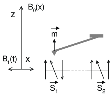
FIG. 1.: Diagram of an MRFM measurement of an entangled state of two spins in a chain of spins. $\vec{S}_{1}$ is a single measured spin which changes its direction under the action of the alternating magnetic field $B_{1}$. ${\vec{S}}_{2}$ is the remote spin entangled with the spin $\vec{S}_{1}$. $\vec{m}$ is the magnetic moment of a ferromagnetic particle which is attached to the cantilever tip. The magnetic force on the cantilever tip (attractive or repulsive) depends on the direction of the spin $\vec{S}_{1}$. $B_{0}$ is the permanent magnetic field which points in the positive $z$-direction.

As an example, we consider a typical entangled state for two spatially separated spins,

$$(1/\sqrt{2})(|\uparrow\uparrow\rangle+|\downarrow\downarrow\rangle).$$

According to the conventional point of view, by measuring the left spin in the state $|\uparrow\rangle$ (or $|\downarrow\rangle$) we automatically collapse a remote right spin into the same state $|\uparrow\rangle$ (or $|\downarrow\rangle$). In the process of MRFM measurement (see Fig. 1) the direction of the measured spin, $\vec{S}_{1}$, changes periodically with the period of the cantilever vibrations. Thus, it is not clear what the direction of the entangled remote spin, $\vec{S}_{2}$, will be after the MRFM measurement.

To study this problem, we simulated the quantum dynamics of this spin-cantilever system assuming that the measuring spin is initially entangled with the remote spin. The remote spin is not subjected to the action of the MRFM apparatus.

The dimensionless quantum Hamiltonian of the spin-cantilever system in the rotating reference frame is [3],

$${\cal H}=(p^{2}_{z}+z^{2})/2+\dot{\varphi}S_{z1}-\epsilon S_{x1}-2\eta zS_{z1}.$$

Here $p_{z}$ and $z$ are the dimensionless momentum and coordinate of the cantilever tip; ${\vec{S}}_{1}$ is the “first” measured spin; $\epsilon=\epsilon(\tau)$ is the dimensionless amplitude of the radio-frequency (rf) field (where $\tau=\omega_{c}t$ is the dimensionless time and $\omega_{c}$ is the cantilever frequency); $\eta$ is the dimensionless constant of interaction between the cantilever and the spin, which is proportional to the magnetic field gradient produced by the ferromagnetic particle on the cantilever tip. The phase of the rf field is taken in the form $(\omega t+\varphi(t))$, where $\omega$ is chosen equal to the Larmor frequency of the spin: $\omega=\omega_{L}$. The time derivative, $\dot{\varphi}$, changes periodically with the frequency of the cantilever vibrations, $\omega_{c}$. In our notation, the dimensionless frequency of the cantilever vibrations is one unit. Thus, the dimensionless period of the cantilever vibrations is $2\pi$. The periodic oscillation of $\dot{\varphi}$ provides a cyclic adiabatic inversion of the spin [4], which drives the resonant vibrations of the cantilever.

The dimensionless wave function of the whole system, including the second entangled spin, can be written in the $z$-representation as,

$$\Psi(z,S_{z1},S_{z2},\tau)=u_{\uparrow\uparrow}(z,\tau)|\uparrow\uparrow\rangle+u_{\uparrow\downarrow}(z,\tau)|\uparrow\downarrow\rangle+$$

$$u_{\downarrow\uparrow}(z,\tau)|\downarrow\uparrow\rangle+u_{\downarrow\downarrow}(z,\tau)|\downarrow\downarrow\rangle.$$

Substituting (3) into the Schrödinger equation, we derive four coupled equations for the functions $u(z,\tau)$,

$$2i\dot{u}_{\uparrow\uparrow}=(p^{2}+z^{2}+\dot{\varphi}-2\eta z)u_{\uparrow\uparrow}-\epsilon u_{\downarrow\uparrow},$$

$$2i\dot{u}_{\downarrow\uparrow}=(p^{2}+z^{2}-\dot{\varphi}+2\eta z)u_{\downarrow\uparrow}-\epsilon u_{\uparrow\uparrow},$$

$$2i\dot{u}_{\uparrow\downarrow}=(p^{2}+z^{2}+\dot{\varphi}-2\eta z)u_{\uparrow\downarrow}-\epsilon u_{\downarrow\downarrow},$$

$$2i\dot{u}_{\downarrow\downarrow}=(p^{2}+z^{2}-\dot{\varphi}+2\eta z)u_{\downarrow\downarrow}-\epsilon u_{\uparrow\downarrow}.$$

This system of equations splits into two independent sets of equations.

FIG. 2.: The probability distribution, $P(z)$, at $\tau=216$.

The initial condition is assumed to be a product of the coherent quasiclassical wave function of the cantilever and the entangled state of the two spins,

$$\Psi(z,S_{z1},S_{z2},0)=(1/\sqrt{2})u_{\alpha}(z)(|\uparrow\uparrow\rangle+|\downarrow\downarrow\rangle),$$

$$u_{\alpha}(z)=\pi^{-1/4}\exp[-(z-\sqrt{2}\alpha)^{2}/2],$$

where $z_{0}\equiv\sqrt{2}\alpha$ is the average initial coordinate of the cantilever. For numerical simulations we used the following values of parameters,

$$\alpha=-10\sqrt{2},~{}\eta=0.3,$$

and the following time dependences for $\epsilon(\tau)$ and $\dot{\varphi}(\tau)$,

$$\epsilon=20\tau,~{}\tau\leq 20;~{}\epsilon=400,~{}\tau>20,$$

$$\dot{\varphi}=-600+30\tau,~{}\tau\leq 20;~{}\dot{\varphi}=1000\sin(\tau-20),~{}\tau>20.$$

The chosen value of $\alpha$ corresponds to the quasiclassical state of the cantilever with the number of excitations $n=|\alpha|^{2}=200$. The chosen value of $\eta$ corresponds to the existing MRFM experiments with electron spins [2]. The time dependences (6) provide the conditions for the cyclic adiabatic inversion of the spin. Fig. 2 shows the typical probability distribution of the cantilever position,

$$P(z)=|u_{\uparrow\uparrow}|^{2}+|u_{\uparrow\downarrow}|^{2}+|u_{\downarrow\uparrow}|^{2}+|u_{\downarrow\downarrow}|^{2}.$$

One can see that the probability distribution, $P(z)$, describes a Schrödinger cat state of the cantilever with two approximately equal peaks. When these two peaks are clearly separated, the total wave function can be represented as a sum of two terms corresponding to the “left” and the “right” peaks in the probability distribution,

$$\Psi(z,S_{z1},S_{z2},\tau)=\Psi_{a}(z,S_{z1},S_{z2},\tau)+\Psi_{b}(z,S_{z1},S_{z2},\tau).$$

Our numerical analysis shows that each term, $\Psi_{a}$ and $\Psi_{b}$, can be approximately decomposed into a direct product of the cantilever and spin wave functions,

$$\Psi_{a}=u_{a}(z,\tau)\chi_{a}(S_{z1},\tau)|\uparrow\rangle_{2},~{}\Psi_{b}=u_{b}(z,\tau)\chi_{b}(S_{z1},\tau)|\downarrow\rangle_{2}.$$

This decomposition is possible because the complex function $u_{\uparrow\uparrow}(z,\tau)$ is proportional to $u_{\downarrow\uparrow}(z,\tau)$, and the complex function $u_{\uparrow\downarrow}(z,\tau)$ is proportional to $u_{\downarrow\downarrow}(z,\tau)$. Such proportionality can be seen in Fig. 3, where we plot the corresponding wave functions at the same time as in Fig. 2, with suitable numerical coefficients.

FIG. 3.: Upper boxes: the real part of wave functions; lower boxes: the imaginary part of wave functions, at $\tau=216$. a)$Re(u_{\uparrow\uparrow})$: solid line; $Re(-5u_{\downarrow\uparrow})$: filled circles. b) $Re(u_{\uparrow\downarrow})$: solid line; $Re(5u_{\downarrow\downarrow})$: filled circles. c) $Im(u_{\uparrow\uparrow})$: solid line; circles $Im(-5u_{\downarrow\uparrow})$filled circles. d) $Im(u_{\uparrow\downarrow})$: solid line; $Im(5u_{\downarrow\downarrow})$: filled circles.

The spin wave function, $\chi_{a}(S_{z1},\tau)$, describes the dynamics of the first spin with its average, $\langle\chi_{a}|\vec{S}|\chi_{a}\rangle$, pointing approximately in the direction of the effective magnetic field, ${\vec{B}}_{\rm eff}$, in the rotating frame,

$$\vec{B}_{\rm eff}=(\epsilon,0,-\dot{\varphi}).$$

(We neglect here the nonlinear term $2\eta z$ whose contribution to the effective field is small.)

FIG. 4.: The positions, $Z_{max}(\tau)$, of two peaks of the Schrödinger cat state as a function of time.

The spin function, $\chi_{b}(S_{z1},\tau)$, describes the dynamics of the first spin with its average pointing in the direction opposite to the direction of $\vec{B}_{\rm eff}$. As the amplitude of the cantilever vibrations increases, the phase difference between the oscillations of the two peaks, $|u_{a}(z,\tau)|^{2}$ and $|u_{b}(z,\tau)|^{2}$, approaches $\pi$. (See Fig. 4.) (To reach the phase difference of $\pi$, a long time of numerical simulations is required. That is why we restricted the simulation time for the results presented in Fig. 4.)

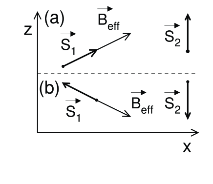
FIG. 5.: Two outcomes of the MRFM measurement of the state of two entangled spins. (a) The measured spin, $\vec{S_{1}}$, points along the direction of the effective magnetic field, and the remote spin, $\vec{S_{2}}$, points “up” (in the positive $z$-direction). (b) The measured spin, $\vec{S_{1}}$, points in the direction opposite to the effective magnetic field, and the remote spin, $\vec{S_{2}}$, points “down” (in the negative $z$-direction).

In realistic experimental conditions, the Schrödinger cat state quickly collapses due to the interaction with the environment [5]. In this case, the two peaks of the probability distribution describe two possible trajectories of the spin-cantilever system. In one of these trajectories the first (measured) spin is pointed along the direction of the effective magnetic field while the second (remote) spin is pointed “up” (in the positive $z$-direction); the other trajectory corresponds to the opposite situation in which the orientation of both spins is reversed—the first (measured) spin is antiparallel to the effective magnetic field, and the second (remote) spin is pointed “down” (in the negative $z$-direction). The phase difference between the corresponding oscillations of the cantilever approaches $\pi$ with increasing cantilever vibration amplitude.

In summary, we have studied the outcome of the MRFM measurement of the entangled spin state, $(1/\sqrt{2})(|\uparrow\uparrow\rangle+|\downarrow\downarrow\rangle)$. Our numerical simulations reveal two possible outcomes shown schematically in Fig. 5: (a) The first (measured) spin points along the effective magnetic field in the rotating frame, and the second (remote) spin points in the positive $z$-direction. (b) The first (measured) spin points opposite to the direction of the effective magnetic field in the rotating frame, and the second (remote) spin points in the negative $z$-direction. Thus, the collapse of the measured spin along (or opposite) the direction of the rotating effective magnetic field leads to the collapse of the remote spin in the positive (or negative) $z$-direction. These two outcomes correspond to two phases of the cantilever vibrations which differ by $\pi$.

This work was supported by the Department of Energy under contract W-7405-ENG-36 and DOE Office of Basic Energy Sciences. The work of GPB, PCH and VIT was partly supported by the National Security Agency (NSA) and by the Advanced Research and Development Activity (ARDA).

REFERENCES

- [1] J.A. Sidles, Appl. Phys. Lett., 58, 2854 (1991).
- [2] D. Rugar, B.C. Stipe, H.J. Mamin, C.S. Yannoni, T.D. Stone, K.Y. Yasumura, T.W. Kenny, App. Phys. A, 72 [Suppl.], S3 (2001).
- [3] G.P. Berman, F. Borgonovi, G. Chapline, S.A. Gurvitz, P.C. Hammel, D.V. Pelekhov, A. Suter, V.I. Tsifrinovich, quant-ph/0101035.
- [4] A. Abraham, Principles of Nuclear Magnitizm, (Oxford University Press, 1961).
- [5] W.H. Zurek, Physics Today, 44, 36 (1991).