Estimation of qubit states in a factorizing basis

Abstract

The optimal estimation of a quantum mechanical 2-state system (qubit) - with $N$ identically prepared qubits available - is obtained by measuring all qubits simultaneously in an entangled basis. We report the experimental estimation of qubits using a succession of $N$ measurements on individual qubits where the measurement basis is changed during the estimation procedure conditioned on the outcome of previous measurements (self-learning estimation). The performance of this adaptive algorithm is compared with other algorithms using measurements in a factorizing basis.

A question of fundamental and practical importance regarding the quantum mechanical description of the microscopic world is: How can we obtain maximal information in order to characterize the state of a quantum system? Quantum states of various physical systems such as light fields, molecular wave packets, motional states of trapped ions and atomic beams have been determined experimentally with considerable precision [1]. Acquiring complete knowledge about a quantum state would, of course, only be possible, if infinitely many copies of a quantum state were available and could be measured. More to the point, the initial question may be reformulated as the following task: Find a procedure consisting of a finite number of measurements yielding a state vector that best represents the (classical) knowledge possibly gained from any type of measurement of the quantum system under scrutiny.

Determining an arbitrary state of a quantum mechanical two-state system (qubit) is of particular importance in the context of quantum information processing. In Ref. [2] two identically prepared 2-state quantum systems were considered with no nonlocal correlations and it was searched for the optimal measurement strategy to gain maximal information (difference of Shannon entropy) about this quantum state. It was strongly suggested that optimal information gain is achieved when a suitable measurement on both particles together is performed. Later it was proven that, indeed the optimal measurement for determining a quantum state - if two spin 1/2 particles are available - needs to be carried out on both particles together, i.e. the operator characterizing the measurement does not factorize into components that act in the Hilbert spaces of individual particles only [3]. Moreover, an optimal estimate of the spin direction (the qubit state) of an ensemble of $N$ identically prepared particles requires the application of such a nonfactorizable measurement operator. As a special case of optimal quantum state estimation of systems of arbitrary finite dimension the upper bound $(N+1)/(N+2)$ for the mean fidelity of an estimate of $N$ qubits was rederived in Ref. [4]. In particular, it was shown that finite positive operator valued measurements (POVMs) are sufficient for optimal state estimation. This result implied that an experimental realization of such measurements is feasible, at least in principle. Subsequently, optimal POVMs were derived to determine the pure state of a qubit with the minimal number of projectors when up to $N=5$ copies of the unknown state are available [5]. Still, the proposed optimal and minimal strategy requires the experimental implementation of rather intricate nonfactorizable operators for a simultaneous measurement on all $N$ qubits. First experimental steps towards entanglement-enhanced determination ($N=2$) of a quantum state have been undertaken [6]. Estimating a quantum state can also be viewed as the decoding procedure at the receiver end of a quantum channel necessary to recover quantum information (e.g. encoded as a unit vector) [7, 8].

It was recently shown that quantum state estimation with fidelity close to the optimum is possible when a self-learning algorithm is used and measurements on $N$ identically prepared qubits are performed separately, even successively [9]. Here, we present, to our knowledge, the first experimental realization of a self-learning measurement on an individual quantum system in order to estimate its state. The base of measurement is varied in real time during a sequence of $N$ measurements conditioned on the results of previous measurements in this sequence. In addition, we compare the attainable experimental fidelity of this adaptive strategy for quantum state estimation with strategies where the measurement base is either a predetermined one, or is randomly chosen during a sequence of $N$ measurements. If a self-learning algorithm is employed to estimate a quantum state, then a suitable target function (here, the gain in the expected mean fidelity as described below) is maximized when proceeding from measurement $n-1$ to $n$. Under realistic experimental conditions possible errors have to be taken into account that may influence different measurement strategies differently.

Here, the quantum mechanical two-state system under investigation is the S_1/2 ground-state hyperfine doublet with total angular momentum $F=0,1$ of a single ¹⁷¹Yb⁺ ion confined in a miniature Paul trap (diameter of 2 mm). The $|0\rangle\equiv|F=0\rangle\leftrightarrow|F=1,m_{F}=0\rangle\equiv|1\rangle$ transition with Bohr frequency $\omega_{0}$ is driven by a quasiresonant microwave (mw) field with angular frequency near $\omega=2\pi\,12.6$ GHz. The system is virtually free of decoherence, i.e. transversal and longitudinal relaxation rates are negligible [10, 11]. Photon-counting resonance fluorescence on the S_1/2(F=1) $\leftrightarrow$ P_1/2(F=0) transition driven by a frequency-doubled Ti:sapphire laser at 369 nm serves for state selective detection. Optical pumping into the $|F=1,m_{F}=\pm 1\rangle$ levels during a detection period is avoided when the E vector of the linearly polarized light subtends 45^o with the direction of the applied dc magnetic field. The light is detuned to the red side of the resonance line by some 20MHz in order to laser-cool the ion. Optical pumping the ion into the metastable ${}^{2}D_{3/2}$ level is prevented by illumination with light at 935 nm of a diode laser that retrieves the ion to the ground state via the $|D_{3/2}$, $F$=$1\rangle\rightarrow|[1/2]_{1/2}$, $F=0\rangle$ excitation. Cooling is achieved by simultaneously irradiating the ion for 100 ms with light from both laser sources and with microwave radiation. This is done before each succession of measurements that consists of preparing and measuring a qubit state $N$ times.

In the reference frame rotating with $\omega$, after applying the rotating wave approximation, the time evolution operator determining the evolution of the qubit exposed to linearly polarized mw radiation reads $U(t)=\exp\left[-\frac{i}{2}t\left(\delta\sigma_{z}+\Omega\sigma_{x}\right)\right]$. The Rabi frequency is denoted by $\Omega$ and $\sigma_{z,x}$ represent the usual Pauli matrices. Any pure state can be represented by a unit vector in 3D configuration space (Bloch vector): $|\theta,\phi\rangle=\cos\frac{\theta}{2}|0\rangle+\sin\frac{\theta}{2}e^{i\phi}|1\rangle$ and is prepared by driving the qubit with mw pulses with appropriately chosen detuning $\delta\equiv\omega_{0}-\omega$, intensity, and duration, and by allowing for free precession for a prescribed time. Rabi frequency ($\Omega=3.47\times 2\pi$ kHz) and detuning ($\delta=107\times 2\pi$ Hz) of the mw radiation are determined by recording Rabi oscillations over 4-8 periods and by performing a Ramsey-type experiment with mw pulses separated in time. A measurement in a given direction is performed in two steps: First, a suitable unitary transformation of the qubit is performed effecting a rotation of the desired measurement axis onto the $z$-axis. Second, the qubit is irradiated for 2 ms with laser light resonant with the S_1/2(F=1) $\leftrightarrow$ P_1/2 transition and scattered photons are detected, if state $|1\rangle$ is occupied.

A self-learning measurement of the prepared qubit state consists of $N$ sequences each comprising i) the preparation of $|\theta_{\rm prep},\phi_{\rm prep}\rangle$, ii) performing a projective measurement in the basis $\left(|\theta_{\rm m},\phi_{\rm m}\rangle_{\rm n}\,,|\bar{\theta}_{\rm m}\equiv\pi-\theta_{\rm m},\bar{\phi}_{\rm m}\equiv\pi+\phi_{\rm m}\rangle_{\rm n}\right)$, and iii) using the result of this $(n-1)^{\rm th}$ measurement to determine the basis of the subsequent $n^{\rm th}$ measurement that maximizes the gain of the expected mean fidelity [9]. This third step will be detailed in what follows.

After $n-1$ sequences the density operator representing the state to be estimated is given by $\varrho_{n-1}=\int_{0}^{\pi}d\theta\sin\theta\int_{0}^{2\pi}d\phi\;w_{n-1}(\theta,\phi)\;|\theta,\phi\rangle\langle\theta,\phi|$. The normalized probability density distribution $w_{n-1}(\theta,\phi)$ is updated after each measurement using Bayes rule [7], i.e. if in sequence $n$ the system is measured in direction $(\theta_{\rm m},\phi_{\rm m})$ the distribution is modified by the probability for this outcome

$$w_{n}(\theta,\phi|\theta_{\rm m},\phi_{\rm m})=\frac{w_{n-1}(\theta,\phi)\;|\langle\theta_{\rm m},\phi_{\rm m}|\theta,\phi\rangle|^{2}}{p_{n}(\theta_{\rm m},\phi_{\rm m})}\;,$$ (1)

where the probability $p_{n}(\theta_{\rm m},\phi_{\rm m})=\langle\theta_{\rm m},\phi_{\rm m}|\varrho_{n-1}|\theta_{\rm m},\phi_{\rm m}\rangle$ to find the system in direction $(\theta_{\rm m},\phi_{\rm m})$ in the $n-$th measurement ensures correct normalization.

The best estimate of the pure qubit state, $|\theta_{\rm est},\phi_{\rm est}\rangle_{n-1}$ is obtained by maximizing the fidelity $F_{n-1}(\theta,\phi)=\langle\theta,\phi|\varrho_{n-1}|\theta,\phi\rangle$, i.e. $F_{n-1}(\theta_{\rm est},\phi_{\rm est})=F^{\rm opt}_{n-1}\equiv\max F_{n-1}(\theta,\phi)$. In order to find the optimal measurement direction for sequence $n$, the expected mean fidelity after measurement $n$ is maximized as a function of the measurement direction. Suppose in the $n$-th measurement the qubit is found in direction $(\theta_{\rm m},\phi_{\rm m})$. Then

$$F_{n}(\theta,\phi|\theta_{\rm m},\phi_{\rm m})=$$ (3)

$$\int_{0}^{\pi}\!d\theta^{\prime}\sin\theta^{\prime}\int_{0}^{2\pi}\!d\phi^{\prime}\,w_{n}(\theta^{\prime},\phi^{\prime}|\theta_{\rm m},\phi_{\rm m})\,|\langle\theta,\phi|\theta^{\prime},\phi^{\prime}\rangle|^{2}\;,$$

where the expected distribution $w_{n}(\theta^{\prime},\phi^{\prime}|\theta_{\rm m},\phi_{\rm m})$ is obtained from Bayes rule (eq. 1). The optimal fidelity $F_{n}^{\rm opt}(\theta_{\rm m},\phi_{\rm m})$ is obtained by maximizing this function with respect to $(\theta,\phi)$. Measurement $n$ is performed along a specific axis and the qubit might as well be found in the direction $(\bar{\theta}_{\rm m},\bar{\phi}_{\rm m})$ Therefore, the expected mean fidelity after the $n-$th measurement is given by the optimized fidelities for each of the two possible outcomes, weighted with the estimated probability for that outcome:

$$\bar{F}_{n}(\theta_{\rm m},\phi_{\rm m})= p_{n}(\theta_{\rm m},\phi_{\rm m})F_{n}^{\rm opt}(\theta_{\rm m},\phi_{\rm m})$$ (4)

$$+ \;p_{n}(\bar{\theta}_{\rm m},\bar{\phi}_{\rm m})F_{n}^{\rm opt}(\bar{\theta}_{\rm m},\bar{\phi}_{\rm m})\;.$$ (5)

The optimal measurement direction $(\theta_{\rm m}^{\rm opt},\phi_{\rm m}^{\rm opt})$ maximizes this function.

The direction of the first ($n=1$) measurement is of course arbitrary, since no a priori information on the state ($w_{0}(\theta,\phi)=\frac{1}{4\pi}$) is available. The expected mean fidelity in this case is $\bar{F}_{1}=2/3$, independent of $(\theta_{\rm m},\phi_{\rm m})_{1}$. After the first measurement the symmetry of the probability distribution $w_{1}(\theta,\phi)$ is reduced to rotational symmetry around the first measurement axis.

The expected mean fidelity now depends only on the relative angle $\alpha$ between the second and the first measurement direction and we find $\bar{F}_{2}=(1/2+\cos(\alpha/2-\pi/4)/\sqrt{18})$. Thus, the optimal second measurement with $\alpha=\pi/2$ yields $\bar{F}_{2}^{\rm opt}=(1/2+1/\sqrt{18})$. After the second measurement $w_{2}(\theta,\phi)$ is still symmetric with respect to a plane spanned by the first two measurements directions. Again, the optimal measurement direction axis is orthogonal to both previous directions and we obtain $\bar{F}_{3}^{\rm opt}=(1/2+1/\sqrt{12})$. The optimal directions of subsequent measurements ($n>3$) do depend on the outcome of previous measurements. For an estimation procedure comprised of $N$ sequences, we have calculated numerically $2^{N}$ possible successions of directions $\{(\theta_{\rm m},\phi_{\rm m})_{n}\}$ and programmed the computer interface that controls the experimental parameters to choose the optimum measurement direction online during an estimation procedure. Fig. 1 illustrates a succession of measurements that yield an estimate of the initial state $|\theta_{\rm prep},\phi_{\rm prep}\rangle=|\pi/4,\pi/4\rangle$ employing the self-learning algorithm. The probability density $w_{n}(\theta,\phi)$ is shown on the surface of the Bloch sphere and the $n^{\rm th}$ and optimized (eq. 5) $(n+1)^{\rm th}$ measurement directions are indicated.

FIG. 1.: Probability distribution $w_{n}(\theta,\phi)$ on the Bloch sphere updated by Bayes rule, in a typical realization of 12 successive measurements. Darker areas correspond to higher probabilities (scaled individually for each Bloch sphere); contour lines for $w_{n}=0,\;0.1,\;\ldots$ are given. The $n^{\rm th}$ and the optimized $(n+1)^{\rm th}$ measurement directions are indicated by the open and the solid arrows respectively. The white circle shows the prepared state $|\theta_{\rm prep},\phi_{\rm prep}\rangle=|\pi/4,\pi/4\rangle$.

The discussion so far is based on the assumption, that measurements are performed with perfect efficiency. This is obviously not true in a real experiment. In this paragraph we will discuss the influence of experimental imperfections on the quality of state estimation. Since the Rabi frequency $\Omega$ and detuning $\delta$ are determined precisely with an error below 1%, the deviation of the prepared state and of the measurement axis from their anticipated directions is small and the resulting systematic error in the fidelity is negligible compared to the statistical error. If there were no background signal during a detection period, the observation of $m>0$ scattered photons in a single measurement would reveal the ion to be in state $|1\rangle$ with probability $1-p_{1}(0)$ close to unity. (The probability $p_{1}(m)$ to detect $m$ photons follows a Poissonian distribution with mean value $\bar{m}_{1}\approx 5$.) However, due to scattering off the ion trap electrodes and windows some photons will be detected even if the ion had been prepared in state $|0\rangle$ (also with a Poissonian distribution $p_{0}(m)$ with $\bar{m}_{0}\approx 0.2$). In order to assign a given number of photon counts in an individual measurement to the corresponding state of the ion, the threshold $s$ is introduced: The probability $\eta_{1}$ to detect $m\geq s$ photons, when photons are scattered off the ion (state $|1\rangle$) is given by $\eta_{1}=\sum_{m=s}^{\infty}p_{1}(m)$. Analogously, $\eta_{0}=\sum_{m=0}^{s-1}p_{0}(m)$ for state $|0\rangle$. The functional relationship between $\eta_{i}$ and $s$ is determined by the observed photon number distributions $p_{i}(m)$. Since the detection efficiencies $\eta_{i}<1$, both a statistical and a systematic error are introduced into the measurements, as will be shown below.

Using the average efficiency $\bar{\eta}\equiv(\eta_{0}+\eta_{1})/2$ and the efficiency difference $\Delta\eta\equiv(\eta_{1}-\eta_{0})/2$, the probability to find an “on” event ($m\geq s$) is given by $P(\mbox{``on"})=(2\bar{\eta}-1)P_{1}+(1-\bar{\eta})+\Delta\eta$, and, analogously $P(\mbox{``off\,"})=(2\bar{\eta}-1)P_{0}+(1-\bar{\eta})-\Delta\eta$, where $P_{i}=|\langle i|\Psi\rangle|^{2}$ and the $|\Psi\rangle$ is the ion’s state before irradiation with UV light. This effect of the measurement can be thought of as the distorting action of a quantum channel on the system’s state followed by a perfect measurement: $\varrho\to(2\bar{\eta}-1)\varrho+(1-\bar{\eta})I+\Delta\eta\;\sigma_{z}$ The channel acts as a depolarizing one characterized by the damping parameter $1-\bar{\eta}$. The error introduced hereby is independent of the choice of the measurement basis and hence statistical. Effectively the purity of the state (or equivalently the length of the Bloch vector $|\langle\vec{\sigma}\rangle|$) decreases. The term in the final density matrix containing $\Delta\eta$ systematically shifts the resulting state along the measurement direction. If an algorithm for state estimation is used that relies on measurements in fixed directions, for example in the $x$,- $y$- and $z$-direction, then the estimated state acquires a component parallel (or anti-parallel for $\Delta\eta<0$) to the direction determined by the vector sum of the measurement directions. On the other hand, algorithms using measurement directions distributed over the whole Bloch sphere tend to cancel this error. This can be achieved with both the self-learning and the random algorithm. For experimental reasons we implemented only measurement directions on the upper hemisphere (i.e. $\theta_{\rm m}\leq\pi/2$) and thus observe this systematic error for all algorithms if $\Delta\eta\neq 0$. Choosing the threshold $s_{\rm opt}$ such that $\Delta\eta=0$ eliminates this systematic, basis dependent error. Whenever an efficiency difference cannot be avoided, any algorithm can be made more robust against a systematic error in the state estimation by choosing measurement directions such that their vector sum is close to zero. Note that $\Delta\eta=0$ (no bias in the estimation procedure) does not, in general, occur at that threshold that is required to make the most probable assignment to state $|0\rangle$ or $|1\rangle$ of a given number of detected photons. The threshold $s^{\prime}_{\rm opt}$ required for the latter would be at the intersection of the two distributions, yielding the maximum of the detection efficiency $\bar{\eta}$. However, the photon count distributions in our experiment yield $s_{\rm opt}=s^{\prime}_{\rm opt}=2$.

We have studied the influence of the bias direction on the performance of all three algorithms. To this end $\Delta\eta$ was varied by changing the threshold $s$ for the estimation of four different prepared states. Each state was estimated several hundred times after 12 consecutive measurements for a given value of $\Delta\eta$. Fig. 2 shows that the dependence of the fidelity on $\Delta\eta$ strongly varies for different states to be estimated. The curves in Fig. 2 intersect where the fidelity is independent of the prepared state. This intersection occurs at $\Delta\eta=0$ as is expected, if the functional dependence of $\Delta\eta$ on $s$ is correct (determined independently using the experimental photon count distributions.)

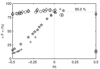
FIG. 2.: Mean fidelity attained with $N=12$ successive measurements, optimized by the self-learning algorithm, as a function of the efficiency difference $\Delta\eta$ for different prepared states (circles: $|3\pi/4,\pi/4\rangle$, diamonds: $|3\pi/4,3\pi/4\rangle$, stars: $|\pi/4,3\pi/4\rangle$, plus: $|\pi/4,\pi/4\rangle$). Each data point is averaged over 100-200 realizations.

In addition to the fidelity optimizing adaptive algorithm, an “orthogonal” and a “random” one have been implemented for comparison. For the orthogonal algorithm equally many measurement are carried out in the $x$- $y$- and $z$- direction. The result of a succession of 4 measurements in each direction is evaluated by updating the probability distribution on the Bloch sphere using Bayes rule as is done for the adaptive algorithm. The random algorithm is realized by employing $2^{N}$ randomly generated directions instead of the $2^{N}$ optimized directions as described above for the self-learning measurement.

Table I shows the fidelities for these three algorithms together with the respective values expected from theory. The experimental fidelities for each algorithm are obtained at the intersection of four curves at $\Delta\eta=0$ corresponding to the estimation of four different initial states as described above. The attainable fidelity is limited by experimental imperfections, i.e. by the finite detection efficiency $\bar{\eta}=97\%$, and most notably by the impure preparation of state $|0\rangle$ at the beginning of each sequence of measurements ($\eta_{\rm prep}=89\%$). The orthogonal algorithm in addition suffered from light-induced decoherence [11]. These imperfections reduce the purity of the state, i.e. the length of the Bloch vector $|\langle\vec{\sigma}\rangle|$. This is accounted for in the theoretical values (table I), that are average values obtained from numerically simulating each algorithm 10.000 times. It should be emphasized that the fidelities given are average values valid for measurement sequences with $N=12$. If instead, the information of all sequences (typically $N\times 100=1200$) is used for state estimation, then the experimental fidelity is better than 99%.

Algorithm	$\langle F\rangle_{\rm Exp.}$	$|\langle\vec{\sigma}\rangle|$	$\langle F\rangle_{\rm Theo.}(|\langle\vec{\sigma}\rangle|)$
self-learning	$85.0\pm 0.6$	$74.8\pm 2.1$	$85.4\pm 0.7$
random	$81.9\pm 0.6$	$73.4\pm 2.1$	$81.9\pm 0.7$
orthogonal	$67.8\pm 1.1$	$40.4\pm 4.6$	$70.2\pm 2.1$
orthogonal		$74.1\qquad\;\>$	$83.6\qquad\;\>$

TABLE I.: Experimental mean fidelities (taken from the data plotted in Fig. 2 at: $\Delta\eta=0$), overall length of Bloch vector $|\langle\vec{\sigma}\rangle|$ and mean fidelities expected from theory, when the length of the Bloch vector is taken into account. For comparison the expected value for the orthogonal algorithm is also given for a $|\langle\vec{\sigma}\rangle|$ as realized with the other algorithms.

The method and results presented are not restricted to a particular realization of qubits. The identification of imperfections in our experiment show that the fidelities obtained are currently limited mainly by the impure preparation. Here, a significant improvement seems feasible: $\eta_{\rm prep}\gtrsim 99\%$ would lead to mean fidelities (with $N=12$ qubits) better than $90\%$, close to the upper bound of $93\%$, attainable with an entangled measurement.

This work was supported by the Deutsche Forschungsgemeinschaft and the Bundesministerium für Forschung und Technologie.

REFERENCES

- [1] For a recent review see, for instance, the special issue on quantum state preparation and measurement, edited by W. P. Schleich and M. Raymer [J. Mod. Opt. 44, No. 11/12 (1997)]; M. Freyberger et al. , Phys. World 10 No.11, 41 (1997); V. Buz̆ek , R. Derka, G. Adam, and P. L. Knight, Ann. Phys. 266, 454 (1998); I. A. Walmsley and L. Waxer, J. Phys. B 31, 1825 (1998); A. White, D. F. V. James, P. H. Eberhard, P. G. Kwiat, Phys. Rev. Lett. 83, 3103 (1999), A. I. Lvovsky et al. . ibid. 87, 050402 (2001).
- [2] A. Peres, W.K. Wootters, Phys. Rev. Lett. 66, 1119 (1991).
- [3] S. Massar, S. Popescu, Phys. Rev. Lett. 74, 1259 (1995).
- [4] R. Derka, V. Buz̆ek, and A. K. Ekert, Phys. Rev. Lett. 80, 1571 (1998).
- [5] J. I. Latorre, P. Pascual, and R. Tarrach, Phys. Rev. Lett. 81, 1351 (1998).
- [6] V. Meyer et al. ,ibid. 86, 5870 (2001).
- [7] K. R. W. Jones, Phys. Rev. A 50, 3682 (1994).
- [8] E. Bagan et al. , Phys. Rev. Lett. 85, 5230 (2000).
- [9] D. G. Fischer, S. H. Kienle, and M. Freyberger, Phys. Rev. A 61, 032306 (2000).
- [10] R. Huesmann et al. , Phys. Rev. Lett. 82, 1611 (1999).
- [11] Ch. Balzer et al. , to appear in Laser Physics at the Limit (Springer, Heidelberg-Berlin-New York, 2001).