Quantum Chaos and Quantum Algorithms

Abstract

It was recently shown (quant-ph/9909074) that parasitic random interactions between the qubits in a quantum computer can induce quantum chaos and put into question the operability of a quantum computer. In this work I investigate whether already the interactions between the qubits introduced with the intention to operate the quantum computer may lead to quantum chaos. The analysis focuses on two well–known quantum algorithms, namely Grover’s search algorithm and the quantum Fourier transform. I show that in both cases the same very unusual combination of signatures from chaotic and from integrable dynamics arises.

The problem of quantum chaos in quantum computers (QC) [1] has recently attracted considerable attention after a pioneering work by Georgeot and Shepelyansky [2]. These authors pointed out that residual, uncontrolled interactions between qubits might induce quantum chaos in the QC if the strength of the interaction exceeds a certain critical level, and they argued that this might destroy the operability of the QC. While the model considered by Georgeot and Shepelyansky [2] does not describe a particular physical realization of a QC, and in particular does not allow for time dependent operating of quantum gates, it is sufficiently generic to mimic a quantum register, i.e. a (static) memory of the QC, in which a state can be stored and from which it should be retrievable again at a later time.

It is clear that residual interactions between the qubits will in general lead to eigenstates of the quantum register that are not the original product states $|0\rangle\ldots|0\rangle|0\rangle$, $|0\rangle\ldots|0\rangle|1\rangle$, $\ldots$ $|1\rangle\ldots|1\rangle|1\rangle$ (called multi–qubit states in the following). Therefore, information stored in the register will evolve with time. If the exact eigenstates of the register are superpositions of only a few multi–qubit states, the register will oscillate quasiperiodically between these. However, in the case of quantum chaos, the eigenstates of the register are superpositions of practically all $2^{n}$ multi–qubit states. The quasiperiodic oscillations due to the interaction between qubits degradate then for all practical times to a decay of the original register state into all multi–qubit states. The time scale $\tau_{\chi}$ for this decay is set by the inverse width of the distribution of eigenenergies. Georgeot and Shepelyansky concluded that all calculations of the quantum computer should have finished long before the time $\tau_{\chi}$ and that this would limit the operability of the computer in a very similar fashion as decoherence. The critical interaction strength $J_{c}$ between qubits at which quantum chaos sets in decreases like $J_{c}\propto 1/n$ with the number $n$ of qubits, and the transition to quantum chaos becomes more and more abrupt with increasing $n$ [2].

Later, Silvestrov et al. questioned Georgeot’s and Shepelyansky’s conclusions [3]. They showed that even in the case of quantum chaos error correction schemes [4, 5] are capable of dealing with errors generated by quantum chaos. However, much more error correction is needed than in the absence of quantum chaos. Their model again included only static interactions between qubits.

In this work I examine a question that is somewhat complementary to the one investigated in [2, 3]: Is it possible that already the interactions introduced on purpose between qubits in order to operate the quantum computer lead to quantum chaos, even if there are no residual parasitic interactions between qubits? This is an intriguing question, since it has implications for the amount of resources necessary for implementing a given algorithm. Already classically chaotic algorithms (e.g. for calculating the time evolution of a classical chaotic system) require much more computing resources than integrable ones: Since errors in the initial conditions amplify exponentially in time, one needs to spend many more bits than for calculating an integrable time evolution over the same time.

In quantum mechanics chaos manifests itself by a sensitivity not to the initial state but to the control parameters [6] (amongst other signatures, see below). The fidelity $|\langle\psi(k)|\tilde{\psi}(k)\rangle|^{2}$ of a wave–function $|\psi(k)\rangle=U^{k}(\lambda)|\psi\rangle$ with respect to a wave–function $|\tilde{\psi}(k)\rangle=U^{k}(\tilde{\lambda})|\psi\rangle$ decreases exponentially with the discrete time $k$, if $\lambda$ and $\tilde{\lambda}$ are two slightly different system control parameters and the time evolution $U(\lambda)$ is chaotic. In the case of integrable quantum dynamics the fidelity typically shows quasiperiodic oscillations in $k$. Therefore a chaotic quantum algorithm will need more resources in the form of more precise quantum gates, or as pointed out in [3], more error correction.

A quantum algorithm (QA) is uniquely defined by the unitary transformation $U$ it induces in the entire multi-qubit Hilbert space, and the question of quantum chaos can be studied directly on the level of that unitary transformation, without the need to deal with the time dependent Hamiltonian by which it is generated. This is what I am going to do in this work, therefore being able to go beyond the models with time-independent Hamiltonians studied in [2, 3].

Obviously, the answer to the question posed depends on the quantum algorithm. A quantum algorithm simulating a quantum chaotic system [7, 8] is by definition a unitary transformation showing quantum chaos, and will thus need very precise tuning of the control parameters. In this paper I focus, however, on two of the most well–known quantum algorithms, where the answer is less clear from the beginning, namely Grover’s search algorithm [9] and the quantum Fourier transform (QFT). The latter is the center piece of several important QAs, like phase estimation, order-finding, the hidden subgroup problem (see [10]), and, most prominently, Shor’s factoring algorithm [11]. Also from the pure quantum chaos point of view the question of quantum chaos in these algorithms is very interesting. In fact it turns out that both algorithms have symmetry properties that lead to a remarkable and very non generic mixture of signatures of quantum chaos and quantum integrability.

The first thing that comes into mind for checking for quantum chaos, is the eigenvalue and eigenvector statistics of $U$: It is believed that an eigenvalue– and eigenvector statistics of $U$ corresponding to Dyson’s circular ensembles indicates quantum chaos [12, 13]. That is, the eigenvalues $\lambda_{i}=\exp(-{\rm i}\varphi_{i})$ should show universal level repulsion [14]. In the limit of large $N$ one expects a distribution $P(s)$ of nearest neighbor spacings $s_{i}=N(\varphi_{i+1}-\varphi_{i})/2\pi$ that is well described by the universal Wigner–Dyson statistics [15]. If $U$ is covariant under any anti–unitary operation $T$ that squares to unity there is always a basis in which the eigenvectors of $U$ can be chosen real. The relevant random matrix ensemble is then the circular orthogonal ensemble (COE) with a $P(s)$ very well approximated by

$$P(s)=\frac{s\pi}{2}{\rm e}^{-s^{2}\pi/4}\,.$$ (1)

The best known example is conventional time reversal symmetry, in which case $T$ is the complex conjugation operator [16]. The eigenvector statistics is usually described in terms of a distribution of eigenvector components. Picking any component $c_{i}$ of any eigenvector at random, random matrix theory (RMT) predicts for $y=N|c_{i}|^{2}$ in the COE case the so–called Porter–Thomas distribution,

$$R_{\rm COE}(y)=\frac{1}{\sqrt{2\pi y}}{\rm e}^{-y/2}\,.$$ (2)

Let us now have a look at Grover’s algorithm [9]. It allows to find an entry with index $\xi$ in a unsorted quantum database that is distinguished from the others by a given property. The distinction may be formalized by an oracle query $O$ which in the multi–qubit basis is a unitary diagonal matrix with entries $O_{ii}=1-2\delta_{i\xi}$ where $\delta_{i\xi}$ is the Kronecker delta. Thus, presented a register state the oracle always gives back the same state unless it is the searched one in which case the oracle changes the state’s phase by $\pi$. Grover’s algorithm commences with the Hadamard transformation

$$H=H_{0}\otimes H_{2}\otimes\ldots\otimes H_{n-1}\,,$$ (3)

where

$$H_{i}=\frac{1}{\sqrt{2}}\left(\begin{array}[]{cc}1&1\\ 1&-1\end{array}\right)$$ (4)

is a Hadamard transformation for the $i$th qubit. Starting from the register state $|0\rangle\ldots|0\rangle$, the Hadamard transformation brings the system into a superposition of all multi–qubit states with equal weight $1/\sqrt{N}$. Next comes an iteration of the oracle query followed by a “diffusion matrix” $D$. The latter has matrix elements $D_{ij}=2/N-\delta_{ij}$. The total algorithm thus reads

$$U_{G}=(DO)^{p}H\,.$$ (5)

The optimal value for the integer $p$ is given by $p=[\pi/(4\theta)]$ with $\sin^{2}\theta=1/N$ ($[.]$ denotes the integer value) [17], and I have chosen this value for all calculations. Remarkably, the quantum computer finds the searched element with $\sim\sqrt{N}$ queries, whereas a classical computer when presented with the same problem would have to ask the oracle on the average $N/2$ times.

From the definition of $U_{G}$ it is clear that $U_{G}$ is real. Covariance under conventional time reversal symmetry,

$$KU_{G}K^{-1}=U_{G}^{\dagger}$$ (6)

thus is fulfilled if $U_{G}$ is symmetric, $U_{G}=U_{G}^{T}$, where $U_{G}^{T}$ denotes the transposed matrix. Using the commutation relations between $H,O$ and $D$ (or by evaluating the matrix numerically, see fig.1) one convinces oneself that $U_{G}$ is almost symmetric.

FIG. 1.: Average absolute value of the matrix elements of the symmetric part of $U_{G}$ (circles) and the antisymmetric part (squares). The former decays like $1/\sqrt{N}$, the latter like $1/N$ where $N={\rm dim_{H}}$ is the dimension of the Hilbert space.

FIG. 2.: Eigenphase spectrum for the Grover algorithm for $q=7$ qubits, $\xi=64$. The spectrum is symmetric and $-\pi$ and $\pi$ should be identified. Only two independent eigenvalues differ from $\pm 1$.

In fact the average absolute value of the matrix elements of the symmetric part of $U_{G}$ decays like $1/\sqrt{N}$, whereas the average absolute value of the antisymmetric part decays like $1/N$. Just one element escapes from the general rule set by the average: $U_{G\xi 0}$, the element in the zeroth column pertaining to the searched element is of order unity minus a $1/\sqrt{N}$ correction (that is how the whole algorithm works), whereas $U_{G0\xi}$ plays no such special role. Nevertheless, for $N\to\infty$ the weight of this particular element is zero and therefore $U_{G}$ has the unusual property that it is at the same time unitary as well as real and (almost) symmetric. Thus, all eigenvalues have to be at the same time on the unit circle, and have to be real. Therefore all eigenvalues are expected to be either unity or minus unity! This is well confirmed numerically (see FIG.2). In fact it turns out that all eigenvalues, even those which are not plus or minus one, are to very good approximation 6th roots of one, and Grover’s algorithm is therefore approximately a 6th root of the unit operation!

The resulting high degeneracy of the eigenphases is in strong contrast to the level repulsion that goes along with quantum chaos. However, absence of level repulsion in $U$ does not exclude quantum chaos. Indeed, suppose some $U$ did show level repulsion, then $U^{M}$ with $M\gg 1$ will in general not, since the spectrum gets completely mixed by winding it $M$ times around the unit circle. A Poissonian statistics will be the consequence. Nevertheless, if $U$ has a chaotic classical counterpart, so will $U^{M}$, and to conclude that $U^{M}$ is not chaotic just from the level statistics is therefore not possible. If the phases of $U$ are commensurate one can even find an $M$ so that all eigenvalues are degenerate.

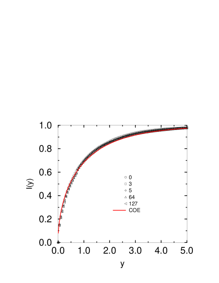
FIG. 3.: Integrated eigenvector distribution $I(y)=\int_{0}^{y}R(x)\,dx$ for the Grover algorithm for $n=7$ and various values of $\xi$. The different symbols denote different selected numbers ($\xi=0,3,5,64$ and 127). The full line is the integrated Porter Thomas distribution.

Let us look at the eigenvector statistics of $U_{G}$. FIG.3 shows that is obeys almost perfectly RMT! This is, however, a pure consequence of the high degeneracy. Indeed, any linear combination of eigenstates in the subspace pertaining to the degenerate eigenvalue $\lambda=1$ is again an eigenstate to the same eigenvalue (and correspondingly for $\lambda=-1$). Thus, a set of eigenvectors can be oriented in a completely arbitrary way in this subspace with the only restriction that they be all normalized and mutually orthonormal. This is just as in RMT, where the eigenvectors are all statistically independent from the eigenvalues, and their orientation is statistically uniform on the whole possible hyper-sphere. In the present situation the diagonalization routine picks initial orientations at random and thus mimics perfect RMT behavior in both of the two subspaces.

Given the unclear picture presented by the eigenvalue and eigenvector statistics, it seems reasonable to examine directly the sensitivity with respect to slight variations in $U_{G}$. One might do so by applying Peres’ original scheme, i.e. creating one perturbed algorithm $U_{G}^{\prime}$ and studying the decay of overlap between $U_{G}^{n}|\psi\rangle$ and $(U_{G}^{\prime})^{n}|\psi\rangle$ as function of $n$ for some random initial $|\psi\rangle$. A natural parameter in $U_{G}$ that might be varied is the number of iterations $p$ of the transformation $DO$. For $p\sim\sqrt{N}$ going from $p$ to $p+1$ appears indeed as a small perturbation. However, all that has been said about the spectrum of $U_{G}$ applies to the such perturbed $U_{G}^{\prime}$ as well, i.e. all eigenvalues will generically be $\pm 1$. A spectral decomposition of $U_{G}=\sum_{i}|u_{i}^{(+)}\rangle\langle u_{i}^{(+)}|-\sum_{l}|u_{l}^{(-)}\rangle\langle u_{l}^{(-)}|+\sum_{k}{\rm e}^{{\rm i}\varphi_{k}}|u_{k}\rangle\langle u_{k}|$ (where $\varphi_{k}$ are the phases different from $0$ and $\pm\pi$) and correspondingly for $U_{G}^{\prime}$ shows that for even $n$ the overlap $\langle\psi|(U_{G}^{\dagger})^{n}(U_{G}^{\prime})^{n}|\psi\rangle$ depends on $n$ only due to the exceptional eigenvalues that differ from $\pm 1$. All the other eigenvalues contribute only two different values to the overlaps, depending on whether $n$ is even or not. Therefore, varying $p$ (or introducing any other perturbation that does not lift the degeneracy of the spectrum) does not lead to exponentially decaying overlap.

I have therefore applied another perturbation: All $DO$ factors in $U_{G}$ are multiplied with a random matrix $V_{i}$ (drawn independently for each factor) close to unity,

$$U_{G}^{\prime}=(DO)V_{1}\ldots(DO)V_{p}H\,.$$ (7)

I constructed all of these random matrices $V_{i}$ as tensor products of $2\times 2$ orthogonal matrices $O(2,\varphi)$ close to ${\rm diag}(1,1)$ in the Hilbert space of each qubit, $V_{i}=O(2,\varphi_{1i})\otimes\ldots\ \otimes O(2,\varphi_{pi})$, where $\varphi_{1i},\ldots,\varphi_{pi}$ are chosen randomly and independently from a uniform distribution in the interval $-\epsilon/2\ldots\epsilon/2$, and $O(2,\varphi)$ is a $2\times 2$ orthogonal transformation acting on a single qubit as

$$O(2,\varphi)=\left(\begin{array}[]{cc}\cos\varphi&\sin\varphi\\ -\sin\varphi&\cos\varphi\end{array}\right)\,.$$ (8)

Fig.4 shows quasiperiodic overlap with almost perfect revival within 500 iterations for a 5 qubit Grover algorithm with $\xi=2$ as selected index and $\epsilon=0.1$. For iteration numbers exceeding 5000 one notices a slight decay, but nevertheless the Fourier spectrum of the decay shows a few very sharp and strong peaks, indicating the quasi-periodic nature of the function. We conclude that according to Peres’ criterion, Grover’s search algorithm is free of quantum chaos.

One might object that as a quantum algorithm, $U_{G}$ will typically not be iterated, though. I therefore also applied another criterion proposed by Schack et al. [18], which seems to be more appropriate in the current situation. These authors examined the distribution of angles between vectors propagated by slightly perturbed unitary matrices, and embedded Peres’ original sensitivity criterion into an information theoretical framework. They showed for the example of a kicked top that in the case of a chaotic quantum map the distribution $P(\alpha)$ of angles $\alpha$ between Hilbert space vectors propagated by many slightly and randomly perturbed unitary transformations corresponds to that of randomly chosen vectors, which resembles a Gaussian peak. An overall average angle can be steered with a deterministic part of the random vectors and adapted to $P(\alpha)$ of the Hilbert space vectors. On the other hand, for integrable quantum maps the random perturbations lead to many more or less degenerate angles, as the propagated vectors do not explore all Hilbert space dimensions. The angle distribution therefore typically contains several more or less pronounced peaks.
FIG. 4.: The overlap between a state propagated by Grover’s algorithm and by a slightly perturbed Grover algorithm ($q=5$ bits, $\xi=2$, $\epsilon=0.1$) plotted on a logarithmic scale. The overlap shows quasiperiodic oscillations, characteristic of integrable behavior.

Instead of adapting the deterministic part of the random vectors, I chose to “unfold” the angles, i.e. to rescale them by the average angle. It turned out that “universal” distributions are obtained by this procedure, both for the randomly drawn vectors as well as those propagated by $U_{G}^{\prime}$. In the latter case one obtains a distribution which over several orders of magnitude of the perturbation strength $\epsilon$ is independent of $\epsilon$, in the former case the unfolded angle distribution is independent of the deterministic part of the random vectors.

I have constructed two particular classes of perturbations. The first one closely corresponds to the original recipe by Schack et al. [18]. The perturbed algorithm is obtained by multiplying all $DO$ factors in $U_{G}$ with only one out of two random orthogonal matrices close to unity, namely $V_{+}=O(2,\varphi_{1})\otimes\ldots\ ,O(2,\varphi_{p})$ or $V_{-}=V_{+}^{-1}$, where again $\varphi_{1},\ldots,\varphi_{p}$ are chosen randomly and independently from a uniform distribution in the interval $-\epsilon/2\ldots\epsilon/2$, but are kept fixed for all factors; i.e. we obtain $2^{p}$ perturbed Grover algorithms $DOV_{+}DOV_{+}\ldots DOV_{+}$, $DOV_{+}DOV_{+}\ldots DOV_{-}$, $\ldots$, $DOV_{-}DOV_{-}\ldots DOV_{-}$. A random initial vector is then propagated by these $2^{p}$ perturbed matrices and the angle distribution between the resulting vectors is analyzed.

Fig. 5 shows that this sort of ’digital’ perturbation does not entirely randomize the propagated vector. Rather the distribution of angles shows many pronounced peaks which means that different perturbations lead to similar Hilbert space vectors. Thus, from this plot one would conclude that the behavior is integrable.
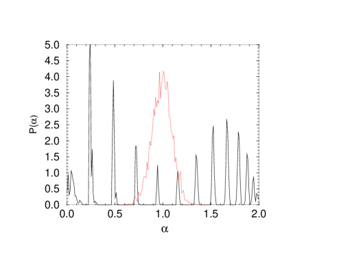
FIG. 5.: The distribution of angles between Hilbert space vectors propagated with $2^{p}$ perturbed Grover algorithms ($q=5$, $\xi=2$, $\epsilon=0.1$ full line) is compared to the distribution of angles between random vectors (dashed line). In both cases the angles were “unfolded” such that the average angles equal unity.
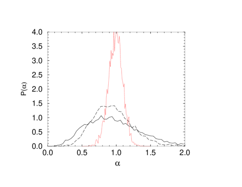
FIG. 6.: The distribution of angles between Hilbert space vectors propagated with 50 perturbed Grover algorithms ($q=5$, $\xi=2$, $\epsilon=0.01$ ; independent random matrices for each factor $DO$, full line) is compared to the distribution of angles between random vectors (narrow peak, dotted line). All angles were “unfolded” such that the average angle is unity. Also shown is the corresponding distribution for the QFT ($q=5$, $\epsilon=0.01$, dashed line).

However, the situation is very different for the second form of perturbation which corresponds to the one introduced for studying the decaying overlap, i.e. instead of choosing between just two matrices $V_{-}$ and $V_{+}$ each factor $DO$ is multiplied with an independent random matrix of the form $V(\varphi_{1i},\ldots,\varphi_{pi})=O(2,\varphi_{1i})\otimes\ldots\,\otimes O(2,\varphi_{pi})$. Fig. 6 shows that in this case a broad, Gaussian like distribution without much further structure arises, much broader in fact (after unfolding) than the angle distribution obtained from the random vectors.

We may therefore conclude that for certain perturbations and according to the criterion by Schack et al. Grover’s search algorithm does show hypersensitivity with respect to perturbations. This is quite surprising in the light of Grover’s earlier finding that almost any unitary transformation substituted for the Hadamard matrix still leads to a functioning search algorithm [19], and it seems, indeed, that the criterion by Schack et al. is singled out compared to the other criteria examined. Note, however, that there is not necessarily a contradiction to Grover’s finding, since for Grover’s algorithm to work it is enough that only the first column of $U_{G}$ be largely unaffected by the perturbations (and the same argument applies to all quantum algorithms that start from just one initial state, typically the state $|00\ldots 0\rangle$)! The present result is more general in as much as it makes a statement about the sensitivity of the entire matrix with respect to perturbations.

How rapidly does the average fidelity decrease with the perturbation strength? If we measure lack of fidelity as average absolute error of all matrix elements, the answer is: linearly, over several orders of magnitude of $\epsilon$ ($0.0001\leq\epsilon\leq 0.1$), as can be seen from Fig.7, and as would have been expected from perturbation theory.

Let me now come to the quantum Fourier transform (QFT). Since it is a universal part of several proposed quantum algorithms including Shor’s algorithm [11], it makes sense to give the QFT special attention. The quantum Fourier transform $U_{FT}$ on a $n$ bit register (with qubits indexed as $0\ldots n-1$) can be constructed from one– and two–qubit operations as [11]

$$U_{\rm FT} = FH_{0}S_{0,1}S_{0,2}\ldots S_{0,n-1}H_{1}\ldots H_{n-3}S_{n-3,n-2}$$ (10)

$$S_{n-3,n-1}H_{n-2}S_{n-2,n-1}H_{n-1}\,,$$

where $S_{j,k}$ is a conditional phase shift matrix between qubits $j,k$ defined by $S_{j,k}={\rm diag}(1,1,1,\exp({\rm i}\pi/2^{k-j}))$ in the basis $00$, $01$, $10$, and $11$ formed by the two qubits $j$ and $k$. The matrix $F$ flips all qubits. With all the two–qubit interactions introduced, one would naively expect quantum chaos. However, the QFT is constructed such that in the whole Hilbert space $U_{\rm FT}$ is very simple and symmetric,

$$U_{{\rm FT}lk}=\frac{1}{\sqrt{N}}{\rm e}^{{\rm i}2\pi lk/N}\,.$$ (11)

One easily convinces oneself that $U^{4}={\bf 1}$! Thus, all possible eigenphases are $0$, $\pi$, and $\pm\pi/2$. The situation is therefore even simpler than in Grover’s algorithm: There is an exact relation that dictates a high degeneracy of only four possible eigenphases. So again, there is no level repulsion.
FIG. 7.: The absolute average error of the matrix elements of Grover’s search algorithm $U_{G}$ (in units of the absolute average matrix element) for random perturbations (independent matrices $V(\varphi)$ for each factor $DO$); $q=5$, $\alpha=2$.

The matrix $U_{\rm FT}$ is covariant under conventional time–reversal: $KU_{\rm FT}K^{-1}=U^{*}=U^{\dagger}$ since $U=U^{T}$. And a numerical evaluation of the eigenvector statistics leads again to good agreement with the Porter–Thomas distribution, which, however, results once more from the high degeneracy of the eigenvalues and not from quantum chaos.
FIG. 8.: The overlap between a state propagated by the QFT and by a slightly perturbed QFT ($q=5$ bits, $\epsilon=0.1$) plotted on a logarithmic scale. The overlap shows quasiperiodic oscillations, characteristic of integrable behavior.

For studying the sensitivity of $U_{\rm FT}$ with respect to perturbations, I slightly perturbed all phases in the conditional phase gates by adding an additional random phase with the same (on the average) relative amount for all gates [21]. Fig. 8 shows that the overlap of a random state propagated with a slightly perturbed matrix $U_{\rm FT}^{\prime}$ and the same state propagated with the original $U_{\rm FT}$ shows again quasiperiodic oscillations. The basic period is two, as could be expected from $(U_{\rm FT}^{2})_{ij}=\delta_{i,N-j}$, i.e. the exact QFT leads back to the same starting vector up to a relabeling of the indices when applied twice. The perturbed QFT only leads to a small deviation from this relabeled initial vector, and therefore almost perfect overlap is restored every second iteration. Thus, according to Peres’ criterion the QFT is free of quantum chaos.

Fig. 6 shows the angle distribution resulting from propagating a random initial vector by 100 differently perturbed matrices for an algorithm running on five qubits. The Hilbert space vectors are complex now, so I defined the angles $\alpha_{i,k}$ as $\alpha_{i,k}=\arccos(|\langle\psi_{i}|\psi_{k}\rangle|/\sqrt{\langle\psi_{i}|\psi_{i}\rangle\langle\psi_{k}|\psi_{k}\rangle})$, and all angles were again rescaled according to $\alpha_{i,k}\longrightarrow\alpha_{i,k}/\langle\alpha\rangle$, where $\langle\alpha\rangle$ is the average angle for all pairs $i\neq k$. The resulting distribution depends for a small number $q$ of qubits still substantially on $q$. For $q=3$ a distribution is obtained that is remarkably close to the famous Wigner Dyson surmise for the orthogonal ensemble (1), but for larger numbers of qubits the distribution approaches more and more a Gaussian, not too different from the distribution obtained from the Grover algorithm (see Fig. 6). Again the distribution is stable in the range I examined it, $0.0001\leq\epsilon\leq 0.1$ . Thus, also the QFT shows hypersensitivity with respect to random perturbations as judged by the criterion of Schack et al., and in contrast to Peres’ original criterion!

On the other hand it is known that if the controlled phase gates are performed to a precision $\Delta=1/p(n)$ where $p$ is a polynomial in the number of qubits, then the maximum error of the final state $U_{QFT}|\psi\rangle$ for all input states $|\psi\rangle$ is of order $n^{2}/p(n)$ [10]. Thus, only polynomial precision is needed for the controlled phase gates. Coppersmith has shown, indeed, that an approximate QFT can be obtained by dropping the gates with the exponentially small phases altogether [22].

In summary I have shown that both Grover’s search algorithm and the QFT give rise to the same unusual combination of quantum signatures of chaos and of integrability. Strong symmetries lead to a large degeneracy of the spectra of eigenvalues of the unitary matrices representing these algorithms. In fact, the QFT is a fourth root of the unity matrix, and Grover’s algorithm is to a good approximation a 6th root of unity! The corresponding lack of level repulsion would be commonly interpreted as absence of quantum chaos. The eigenvector statistics closely follows RMT predictions, and one would commonly interprete this as a signature of quantum chaos. However, as shown above, it is here but an artefact arising from the highly degenerate spectrum. The overlap between a random state propagated by a perturbed algorithm and the same state propagated by the corresponding unperturbed algorithm shows quasiperiodic oscillations both for Grover’s algorithm and the QFT, thus signaling absence of quantum chaos, in agreement with earlier studies addressing the stability of these codes. The only criterion indicating quantum chaos and not evidently explainable by an artefact is the distribution of angles between vectors propagated once by many slightly disturbed algorithms. After unfolding the angles universal distributions are obtained for large enough Hilbert spaces, both for Grover’s algorithm and for the QFT, that resemble the one for random vectors.

Acknowledgment: I would like to thank Henning Schomerus for a useful discussion. This work was supported by the Sonderforschungsbereich 237 “Unordnung und große Fluktuationen”.

REFERENCES

- [1] D. Deutsch, Proc. R. Soc. A 400, 97 (1985); ibid., 425, 73 (1989).
- [2] B. Georgeot and D. L. Shepelyansky, quant-ph/9909074 nad quant-ph/0005015. D. L. Shepelyansky, quant-ph/0006073.
- [3] P. G. Silvestrov, H. Schomerus, and C. W. J. Beenakker, quant-ph/0012119.
- [4] P. W.Shor, Phys. Rev. A 52, 2493 (1995).
- [5] A. M. Steane, Phys. Rev.Lett. 77, 793 (1996).
- [6] A. Peres in Quantum Chaos, ed. by H. A. Cerdeira, R. Ramaswamy, M. C. Gutzwiller, and G. Casati (World Scientific, Singapore, 1991).
- [7] P. H. Song and D. L. Shepelyansky, Phys. Rev. Lett. 86, 2162 (2001).
- [8] B. Georgeot and D. L. Shepelyansky, Phys. Rev. Lett. 86, 2890 (2001).
- [9] L. K. Grover, Phys. Rev. Lett. 79, 325 (1997).
- [10] M. A. Nielsen and I. L. Chuang, Quantum Computation and Quantum Information, Cambridge University Press, Cambridge, UK (2000).
- [11] P. W. Shor in Proc. 35th Annual Symp. on Foundations of Computer Science (Santa Fe, NM: IEEE Computer Society Press); see also quant-ph/9508027.
- [12] O. Bohigas, M. J. Giannoni and C. Schmitt, Phys.Rev.Lett 52, 1 (1984).
- [13] M.V.Berry and M.Robnik, J.Phys.A: Math.Gen.17, 2413 (1984).
- [14] No definitive proof of this so–called RMT–hypothesis is known, but overwhelming experimental and numerical evidence exists (see T. Guhr A. Müller–Gröling, H.A. Weidenmüller, Phys.Rep.299, 190 (1998)). Recently a strong analytical argument has been found (P.A.Braun, S. Gnutzmann, F. Haake, M. Kus, K. Życzkowski; nlin.CD/0006022).
- [15] M.L. Mehta, Ramdom Matrices, 2nd edn. (Academic Press, New York, 1991).
- [16] F. Haake, Quantum Signatures of Chaos, Springer, Berlin (1991).
- [17] M. Boyer, G. Brassard, P. Hoyer, and A. Tapp, in Proceedings of the 4th Workshop on Physics and Computation — PhysComp’96 (1996); quant-ph/9605034.
- [18] R. Schack, G. M. D’Ariano, and C. M. Caves, Phys. Rev. E 50, 972 (1994).
- [19] L.K. Grover, Phys.Rev.Lett. 80 4329 (1998).
- [20] D. A. Lidar and O. Biham, Phys. Rev. E 56 3661 (1997).
- [21] Note that the original phases vary between and , so perturbing with the same relative error is essential.
- [22] D. Coppersmith, IBM Research Report RC 19642.