Decoherence for classically chaotic quantum maps

Abstract

We study the behavior of an open quantum system, with an $N$–dimensional space of states, whose density matrix evolves according to a non–unitary map defined in two steps: A unitary step, where the system evolves with an evolution operator obtained by quantizing a classically chaotic map (baker’s and Harper’s map are the two examples we consider). A non–unitary step where the evolution operator for the density matrix mimics the effect of diffusion in the semiclassical (large $N$) limit. The process of decoherence and the transition from quantum to classical behavior are analyzed in detail by means of numerical and analitic tools. The existence of a regime where the entropy grows with a rate which is independent of the strength of the diffusion coefficient is demonstrated. The nature of the processes that determine the production of entropy is analyzed.

I Introduction

Decoherence has been recognized in recent years as one of the main ingredients needed to understand the origin of the classical world from the fundamental quantum laws [1, 2]. Decoherence is a process whose origin is conceptually simple: It is due to the entanglement between the system and its environment that is created in the course of their interaction. As a consequence, the environment keeps a record of the state of the system, that loses its purity. Only a small subset of all possible states of the system (the so–called pointer states) are relatively stable against the interaction. They are the ones which are less likely to become entangled with the environment. In the vast majority of cases, when the state is a superposition of pointer states, the information initially stored in the state of the system can never be restored since it irreversibly flows into the correlations with the environment. A basic question one should ask in this context is how fast does the information flow away from the system. This can be studied, for example, by analyzing the evolution of the entropy obtained from the reduced density matrix of the system. This has been done for a variety of cases (see [2] for a review) and it has been recognized that this process has unique features if the system has a classically chaotic counterpart. In fact, as conjectured in [3, 4], the rate of entropy production in such cases has a regime that is independent of the strength of the coupling between the system and the environment and is entirely determined by the dynamical parameters characterizing the chaotic evolution. This conjecture was analyzed in the literature mostly using numerical tools [5, 6, 7, 8, 9, 10, 11]. In this paper we will present a study of this problem for some systems that are simple enough to enable both a rigorous numerical treatment and some analytic estimates. We consider here a quantum system with a finite dimensional Hilbert space ($N$ is the number of dimensions, and we are interested in learning about the behavior of the system in the large $N$ limit). For such system we define an evolution operator for the density matrix in two steps as follows: first we consider a purely unitary evolution defining an operator $U$ which is such that it corresponds (in the large $N$ limit) to a classically chaotic map. Then, we define a non–unitary map for the density matrix in such a way that (again, in the large $N$ limit) it mimics the effect of the interaction with an environment producing the same effects one observes for a Brownian particle (namely, diffusion). For such system, we developed a numerical code enabling us to efficiently evolve the density matrix and study in particular the evolution of the entropy. Our aim is to present solid numerical evidence supporting the conjecture presented in [3, 4] and, by combining the numerical work with analytic calculations, develop new intuition on the main processes contributing to entropy production for this kind of systems.

The paper is organized as follows: In Section II we review some basic elements of the theory of quantum maps. We focus, as in the rest of the paper, on two specific examples: baker’s map (the paradigmatic example of a fully chaotic system) and Harper’s map (an example of the wide class of kicked maps with mixed phase space). There are no new results presented in this section and the reader with experience in the theory of quantum maps can easily skip it. In Section III we describe in detail the model for decoherence that we study in this paper. In Section IV we present the main results concerning the behavior of the entropy as a function of time and the evolution of the Wigner function. Finally, in Section IV we present our conclusions. An Appendix contains technical details about the phase space representation we use in this paper (the discrete Wigner function).

II Quantum Maps

The construction of the quantum analogue of a classical map follows two well defined steps : a kinematical one, where the nature of the Hilbert space is defined in relationship with a specific phase space structure, and a dynamical one, where a unitary operator defines the evolution for a finite time step. For the study of chaotic behaviour, a finite phase space is required and therefore the question of boundary conditions arise. The simplest case is the torus, where periodic boundary conditions are assumed for both the coordinate and momentum representations. The most general quasi-periodic boundary conditions are

$$\langle{q+1}|{\psi}\rangle = e^{i2\pi\chi_{q}}\langle{q}|{\psi}\rangle$$ (1)

$$\langle{p+1}|{\psi}\rangle = e^{-i2\pi\chi_{p}}\langle{p}|{\psi}\rangle$$ (2)

where $\chi_{q}$ and $\chi_{p}$ are fixed, arbitrary real numbers between $0$ and $1$ ($2\pi\chi_{q}$ and $2\pi\chi_{p}$ are called Floquet angles). These conditions result in a finite dimensional Hilbert space. This space’s dimension, $N$, is related to $\hbar$ by the relation

$$2\pi\hbar N=1$$ (3)

which signifies that phase space (of area equal to unity ) is spanned by $N$ states (of area $2\pi\hbar$). The position and momemntum eigenvalues in this finite dimensional space are

$$|{q_{n}}\rangle = |{\frac{n+\chi_{p}}{N}}\rangle,\quad n=0,1,\dots,N-1,$$ (4)

$$|{p_{m}}\rangle = |{\frac{m+\chi_{q}}{N}}\rangle,\quad m=0,1,\dots,N-1.$$ (5)

These position and momentum eigenstates are related by a discrete Fourier transform:

$$\langle{p_{m}}|{q_{n}}\rangle=\frac{1}{\sqrt{N}}e^{-i\frac{2\pi}{N}(m+\chi_{q})(n+\chi_{p})}\equiv\left(G_{N}^{\chi_{q},\chi_{p}}\right)_{mn}$$ (6)

The values of $\chi_{q}$ and $\chi_{p}$ specify different Hilbert spaces. In the present paper we will use $\chi_{q}=\chi_{p}=\frac{1}{2}$, corresponding to antiperiodic boundary conditions. Cyclic shifts on these two bases are implemented by unitary operators [12]

$$\hat{\cal U}|{q_{n}}\rangle = |{q_{n+1}}\rangle$$ (7)

$$\hat{\cal V}|{p_{m}}\rangle = |{p_{m+1}}\rangle.$$ (8)

These operators and their powers can be combined to produce unitary displacement operators in phase space

$$\hat{D}(\Delta p,\Delta q)=\hat{\cal U}^{\Delta q}\hat{\cal V}^{\Delta p}e^{i{\frac{\pi}{N}\Delta p\Delta q}}$$ (9)

for integer values of $\Delta p,\Delta p$. These are the analogues of the Weyl displacement operators in the continuous case. Phase space in this context is then assimilated to a discrete $N\times N$ grid which will be useful for the representation of quantum effects in phase space (see Appendix).

A The baker’s map

The baker’s map is one of the simplest systems displaying strongly chaotic behaviour. In spite of its simplicity, it has a very rich dynamical behaviour, both in its classical and its quantum versions. The map is an area preserving transformation defined in the $[0,1]\times[0,1]$ phase-space square as:

$$q^{\prime} = 2q-[2q]$$ (10)

$$p^{\prime} = \frac{1}{2}(p+[2q])$$ (11)

where the square brackets symbolize the integer part of a real number. This evolution has a very simple geometrical interpretation, as a ”stretching” step followed by “cutting” step, as a baker rolling dough. The map is uniformly hyperbolic, with a single Lyapunov exponent, with a value of $\ln 2$. Moreover, at every point the stable and unstable manifolds are parallel to the coordinate axes. The baker’s map has a remarkably simple symbolic dynamics, and can be mapped into an unrestricted Bernoulli shift on two symbols [13]. If the phase space coordinates $p$ and $q$ are written in binary notation

$$q=0.\epsilon_{0}\epsilon_{1}\epsilon_{2}\epsilon_{3}\dots\quad\quad p=0.\epsilon_{-1}\epsilon_{-2}\epsilon_{-3}\epsilon_{-4}\dots$$ (12)

$$(p,q)=\dots\epsilon_{-4}\epsilon_{-3}\epsilon_{-2}\epsilon_{-1}\bullet\epsilon_{0}\epsilon_{1}\epsilon_{2}\epsilon_{3}\dots$$ (13)

The map’s action on these symbols is to move the most significant bit of $q$ to $p$, shifting to the right the decimal point in $q$:

$$q^{\prime}=0.\epsilon_{1}\epsilon_{2}\epsilon_{3}\dots\quad\quad p^{\prime}=0.\epsilon_{0}\epsilon_{-1}\epsilon_{-2}\epsilon_{-3}\dots$$ (14)

$$(p^{\prime},q^{\prime})=\dots\epsilon_{-4}\epsilon_{-3}\epsilon_{-2}\epsilon_{-1}\epsilon_{0}\bullet\epsilon_{1}\epsilon_{2}\epsilon_{3}\dots$$ (15)

Thus each doubly infinite sequence of binary digits represents a unique trajectory. The phase space points on this trajectory are obtained by placing the dot somewhere (the present) and reading off the coordinate and momentum to the right and left of it.

The quantization procedure for the map is not unique but follows closely semiclassical prescriptions. As originally formulated [14] it used periodic boundary conditions ($\chi_{q}=\chi_{p}=0$) but was later modified to antiperiodic conditions ($\chi_{q}=\chi_{p}=\frac{1}{2}$) [15]. The full semiclassical theory has been developed in [16]. The resulting unitary matrix for one step of the map is

$$\hat{B}_{baker}=\hat{G}_{2N}^{-1}\left[\begin{array}[]{cc}\hat{G}_{N}&0\\ 0&\hat{G}_{N}\\ \end{array}\right]$$ (16)

A different approach, leading to the same result, was proposed in [17] (see also [18]) interpreting the map as the quantization of a Bernouilli shift showing that it could be implemented by elementary gates and thus would be an interesting candidate to be run as an algorithm in a quantum computer. This approach is strongly based on the symbolic dynamics of the map and runs as follows: as the position and momentum basis are related by a Fourier transform, we can implement the Bernoulli shift - which shifts the most significant bit of the coordinate to the most significant bit of momentum - using the quantum circuit shown in figure 1.

FIG. 1.: Quantum circuit which perform a Bernoulli shift, i.e. an iteration of the quantum baker’s map

The action of this circuit can be understood as follows: the qubits on the input codify in the usual way the eigenvalues of the position operator with the most significant bit at the bottom; after applying the split Fourier transform, the most significant qubit now represents the most significant bit of the eigenvalue of the momentum operator. As a final step, an inverse Fourier transform allows us to look at the final state in the position basis. This is exactly the circuit representation of the matrix $\hat{B}_{baker}$ . As is well known [19] the Fourier matrices can be further decomposed into elementary gates leading to a circuit representation in terms of operations on qubits.

B The Harper’s map

The baker’s map does not capture the full complexity of chaotic motion in Hamiltonian systems. The fact that it has uniform hyperbolicity and very simple manifolds are not very generic properties as the most common situation is that of a complex mixture of elliptic islands interspersed by chaotic regions with locally defined Lyapounov exponents. To address this more general situation a different family of maps can be devised whose characteristic is to alternately produce “kicks” of potential or kinetic energy. The combined action of these kicks is equivalent to that of a periodic time dependent Hamiltonian and the resulting motion is area preserving and can mimic the full complexity of a generic system. A wide variety of maps on the sphere (kicked tops), on the cylinder (kicked rotors), or on the torus (Harper’s map) have been extensively studied in the quantum chaos literature [20, 21].

Here we have studied a specific kicked map, known as the Harper’s map because of its relationship to the Harper’s hamiltonian in solid state physics. This map acts on the unit square with periodic boundary conditions in phase-space and is defined by the transformation [21]

$$q^{\prime} = q-\gamma\sin(2\pi p)\quad(\mathop{\operator@font mod}\nolimits 1)$$ (17)

$$p^{\prime} = p+\gamma\sin(2\pi q^{\prime})\quad(\mathop{\operator@font mod}\nolimits 1).$$ (18)

The behaviour of the map is determined by the real parameter $\gamma$. If $\gamma\ll 1$ the map approaches an infinitesimal transformation with approximately conserved energy and its evolution is regular. If, on the other hand, $\gamma\approx 1$ the map becomes fully chaotic. In between, the motion presents the complex mixture of regular and chaotic motion characteristic of most realistic systems.

The reason that kicked maps are so popular is that they are very easy to quantize. In fact the potential and the kinetic kicks are respectively diagonal in the coordinate and momentum basis and therefore the full evolution consists of these diagonal kicks interspersed by the Fourier transformation between these two bases. One full step of the map is then the evolution operator $\hat{U}$,

$$\hat{U}=\hat{U}_{q}\hat{G}^{\dagger}_{N}\hat{U}_{p}\hat{G}_{N}$$ (19)

For the Harper’s map the two diagonal operators $\hat{U_{q}}$ and $\hat{U}_{p}$ are

$$\hat{U}_{q}|{q_{n}}\rangle = e^{-i{\gamma N\cos(\frac{2\pi}{N}(n+\chi_{p}))}}|{q_{n}}\rangle$$ (20)

$$\hat{U}_{p}|{p_{k}}\rangle = e^{-i{\gamma N\cos(\frac{2\pi}{N}(k+\chi_{q}))}}|{p_{k}}\rangle$$ (21)

and $\hat{G_{N}}$ is given by (6).

Kicked maps also lead very naturally to a circuit interpretation, like in the case of the baker’s map. The diagonal interactions are controlled phases that act among all the qubits while the Fourier transformations can again be decomposed into elementary gates. Some of these maps (the cat maps, for example) can be efficiently decomposed in terms of elementary operatios and have recently been studied as possible candidates to be simulated in a quantum computer [22]. Figure 2 shows the structure of a quantum circuit which implements a generic kicked map.

FIG. 2.: Quantum circuit which implements a quantum kicked map.

III Dissipative maps

Our aim is to study the impact of the process of decoherence induced by the interaction between our system and an external environment. The system would otherwise evolve according to one of the unitary operators described in the previous section. In general, modeling the coupling to the outside world may be complicated. Here, we will not use a microscopic model of this interaction but will describe the effect of the environment in a phenomenological way by defining a dissipative map for the evolution of the density matrix of the system. As decoherence generally induces a loss of purity, the first important point to notice is that the state of the system should be defined in terms of a density matrix $\rho$. In the absence of any coupling to the environment, the density matrix $\rho$ evolves unitarily according to the map

$$\hat{\rho}^{\prime}=\hat{U}\hat{\rho}\hat{U}^{\dagger}.$$ (22)

The coupling to the environment would induce nonunitary evolution. To correspond to an allowed temporal evolution (that should come from a unitary map for the whole Universe), the nonunitary map for the density matrix has to satisfy some constraints. Assuming that: i) it is linear and preserves hermiticity, ii) it is trace preserving and iii) it preserves the complete positivity of the density matrix [19]; the map is strongly constrained. Moreover, if one imposes also Markovian behavior (neglecting all memory effects) one can show that the most general map for the density matrix of the system should be of the form:

$$\hat{\rho}^{\prime}=\sum_{k}\hat{E}_{k}\hat{\rho}\hat{E}^{\dagger}_{k}$$ (23)

Equation (23) is known as the operator sum representation (or Kraus representation) of the superoperator which maps $\hat{\rho}$ onto $\hat{\rho}^{\prime}=\$(\hat{\rho})$ (see [19, 23, 24] for a review of this representation and a derivation of the main formulae). The trace preserving nature of the superoperator defines a constraint for the operators $\hat{E}_{k}$:

$$\sum_{k}\hat{E}^{\dagger}_{k}\hat{E}_{k}=\hat{I},$$ (24)

where $\hat{I}$ is the identity operator. There is no other constraint on these operators, although it is worth noting that this constraint boils down to plain unitarity if there is only one operator. There is a nice physical interpretation for the $\left\{{\hat{E}_{k}}\right\}$ operators: One can think equation (23) as corresponding to a process where the state $\hat{\rho}$ is converted randomly into the state $\frac{\hat{E}_{k}\hat{\rho}\hat{E}^{\dagger}_{k}}{\mathop{\operator@font tr}\nolimits\left(\hat{E}_{k}\hat{\rho}\hat{E}^{\dagger}_{k}\right)}$ with a probability $\mathop{\operator@font tr}\nolimits\left(\hat{E}_{k}\hat{\rho}\hat{E}^{\dagger}_{k}\right)$ (in this sense, these operators are quantum jump operators). It is important to notice that the set of the $\hat{E}_{k}$ corresponding to a given non-unitary evolution is not unique: For example, if $U_{kl}$ are the elements of a unitary matrix, we can define the operators $\hat{E}_{l}^{\prime}$ as

$$\hat{E}^{\prime}_{l}=\sum_{k}U_{kl}\hat{E}_{k},$$ (25)

and show that the set $\left\{{\hat{E}_{l}^{\prime}}\right\}$ generates the same evolution as the set $\left\{{\hat{E}_{l}^{\prime}}\right\}$.

We will use the operator sum representation to define a specific model to introduce decoherence in our system. We want our model to correspond, in the continuum limit (where $N\rightarrow\infty$) to a diffusive environment having similar effects than the ones present in the well studied Brownian motion model [25]. For this, we will assume that the temporal evolution is divided in two steps: a unitary step, where the density matrix evolves unitarily as in (22); and a dissipative step, where the density matrix evolves by a map whose operator sum representation is of the form:

$$\hat{\rho}^{\prime}=(1-\alpha)\hat{\rho}+\frac{\alpha}{2}(\hat{D}(\Delta q,\Delta p)\hat{\rho}\hat{D}^{\dagger}(\Delta q,\Delta p)+\hat{D}^{\dagger}(\Delta q,\Delta p)\hat{\rho}\hat{D}(\Delta q,\Delta p)).$$ (26)

where $\alpha$ is a real number between $0$ and $1$ measuring the strength of the coupling to the environment and $\hat{D}(\Delta q,\Delta p)$ is the displacement operator defined in (9), which from now on will be denoted simply as $\hat{D}$. Notice the constraint (24) is automatically satisfied because $\hat{D}$ is unitary. In fact, in the above equation the three terms appearing in the operator sum representation are:

$$\hat{E}_{0} = \sqrt{(1-\alpha)}\hat{I}$$ (27)

$$\hat{E}_{1} = \sqrt{\frac{\alpha}{2}}\hat{D}$$ (28)

$$\hat{E}_{2} = \sqrt{\frac{\alpha}{2}}\hat{D}^{\dagger},$$ (29)

which are normalized in such a way that (24) holds.

The above operator sum representation provides an intuitive interpretation for the evolution: the density matrix is first evolved with the unitary quantum map (the unitary step). Then, three things can happen: i) with probability $1-\alpha$ the state does not change; ii) with probability $\frac{\alpha}{2}$ the state is displaced in one direction in phase space; iii) with probability $\frac{\alpha}{2}$ the state is displaced in the opposite direction in phase space. As the probabilities of both displacements are equal, a localized state does not drift in phase space as a consequence of this evolution. The net effect is to smear the state in phase space in the direction of the displacement operator. Thus, this nonunitary map is a discrete model for a diffusive process. The diffusive superoperator can be made a more efficient by using not just a single displacement operator but rather a sum of many terms. Thus, we will consider a more general model where

$$\hat{\rho}^{\prime}=(1-\alpha)\hat{\rho}+\frac{\alpha}{2M}\sum_{n=1}^{M}(\hat{D_{n}}\hat{\rho}\hat{D_{n}}^{\dagger}+\hat{D_{n}}^{\dagger}\hat{\rho}\hat{D_{n}})$$ (30)

where $\hat{D_{n}}=\hat{D}(\Delta q_{n},\Delta p_{n})$ for some displacements $\Delta q_{n}$ and $\Delta p_{n}$. In particular, it is simplest to consider all displacements along the same direction (i.e. $\Delta q_{n}=n\Delta q$ and $\Delta p_{n}=n\Delta p$). In such case, we can get the following formula for the evolution of the matrix elements of $\hat{\rho}$ (in the basis of eigenstates of $\hat{D_{n}}$):

$$\frac{\langle{i^{\prime}}|\hat{\rho}^{\prime}|{i}\rangle}{\langle{i^{\prime}}|\hat{\rho}|{i}\rangle}=1-\alpha\big{[}1-\cos(\frac{\pi(i-i^{\prime})}{N}(M+1))\frac{\sin(\frac{\pi(i-i^{\prime})}{N}M)}{M\sin(\frac{\pi(i-i^{\prime})}{N})}\big{]}$$ (31)

From this equation we see that the effect on the density matrix in this representation is clear: the diagonal elements are unaffected by the non–unitary evolution while the non-diagonal elements are suppressed by a factor that rapidly decays with the distance to the diagonal. In the continuous case this suppression is gaussian [20] but here, due to the discreteness of the Hilbert space the suppression has the shape of a diffraction-like kernel. Using the above expression it can be shown that if $M=N$, the net effect of one step is to completely wipe out all the non-diagonal elements, leaving a diagonal density matrix.

The diffusive character of this non–unitary map is even clearer if we represent the quantum state in phase space using the Wigner functions. As we are dealing with a finite dimensional Hilbert space we should use a discrete version of the ordinary Wigner function which is well adapted to the finite phase space structure [26]. The definition and main properties are given in the Appendix and more in detail in Ref.[27]. In this representation the Wigner function of the density operator is a real array defined on a $2N\times 2N$ lattice in phase space which shares many of the well known properties of the continuous Wigner function. The action of the diffusive map given in equation (30) in the Wigner representations is

$$W^{\prime}(q,p)=(1-\alpha)W(q,p)+\frac{\alpha}{2M}\sum_{n=1}^{M}[W(q+2n\Delta q,p+2n\Delta p)+W(q-2n\Delta q,p-2n\Delta p)]$$ (32)

This expression shows clearly that the diffusive step smears the Wigner function in directions specified by $\Delta p,\Delta q$ (the factor of $2$ present in the above equation is due to the fact that the phase space is an array of size $2N\times 2N$ rather than $N\times N$). More general diffusion models involving mixtures in different directions in phase space, or even over whole areas where diffusion occurs are similarly represented.

IV Results

In this section we present and discuss our results. They concern two separate but connected issues: First, we will examin the behavior of entropy as a function of time focusing both on understanding the role of the different mechanisms that make entropy to grow and determining the dependence of the rate at which it grows on the parameters of our model (like the strength of the coupling, etc). Second, we analize the issue of the correspondence between quantum and classical dynamics. The basic tool we used for our studies is a highly efficient code to evolve the density matrix which makes good use of fast Fourier transform routines. With this, running on a PC, one can easily compute the density matrix for Hilbert spaces with dimension of about $N=2000$ (larger machines would be required to go above that limit but there is no good reason to do that, see below). The source code is available from the authors.

A Rate of entropy production

For a variety of initial states we studied the evolution of the density matrix under the dissipative map and computed the linear entropy $S=-\log(Tr(\rho^{2}))$. We did that both for the baker’s and the Harper’s map. The diffusion mechanism is as in (30) and in the plots $\alpha_{p}$ labels diffusion along the momentum axis ($\hat{D}=\hat{\cal V}$ ) while $\alpha_{q}$ labels diffusion along the coordinate ($\hat{D}=\hat{\cal U}$) Our results clearly establish that in both cases, the rate of entropy production becomes independent of the parameter $\alpha$ provided its value is above a certain threshold (that is close to $0.4$). This is seen in Figures 3 where the plots show the entropy as a function of time for two types of diffusive environments (where diffusion is along either position or momentum). It stands out from this graph that all of the curves with $\alpha$ greater than $0.4$ have a linear regime with the same slope. This slope turns out to be equal to $\ln 2$, the Lyapunov exponent for the baker’s map.

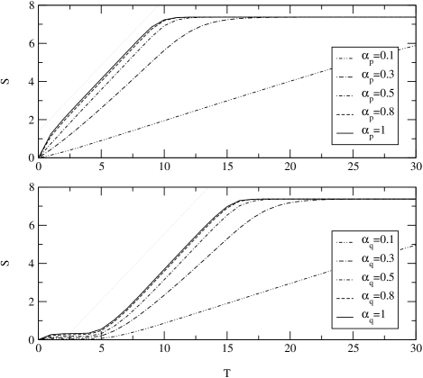
FIG. 3.: Linear entropy growth for the baker’s map with N=1594 and different values for $\alpha$. For the top graph diffusion is along momentum and for the bottom graph along position.

Similar results are shown in Figure 4, for which the unitary propagation was provided by the Harper map. Even though in this case there is not a well defined linear regime (at least not so well defined as in the case of the baker’s map), it is clear that the rate of entropy production becomes independent of $\alpha$. Thus, in this regime entropy is produced due to the coupling with the environment but the rate becomes independent of the coupling strength.

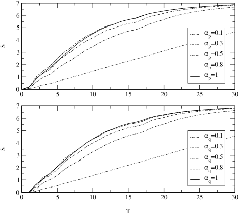
FIG. 4.: Same as Fig 3 but for Harper’s map ($\gamma$ = 0.45)

This is one of the main results of the paper, that substanciates the conjecture that was originally put forward in [3] and later tested numerically in various works [5, 9, 10].

We have also studied the dependence of the entropy growth as a function of $N$ (the dimensionality of the Hilbert space). This was done both for small values of $\alpha$ and in the regime where the rate of entropy production is independent of the coupling. These results are shown in Figures 5 and 6. In both cases we have found that - when appropriately rescaled - the entropy growth is quite independent on the value of $N$ and tends to a universal curve in the limit $N\to\infty$ (as $1/N$ is the effective Planck constant this corresponds to the classical limit). This result suggests that the mechanism for entropy growth in quantum maps has a dominant classical component with corrections that vanish in the classical limit.

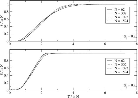
FIG. 5.: Scaling of the linear entropy growth with dimension of the Hilbert space of the system with diffusion on the position axis. The strength of the diffusion is kept constant by smoothing over a constant fraction of the system’s phase space. In relationship with Figures 5 and 6 both axis have been rescaled by $\log(N)$

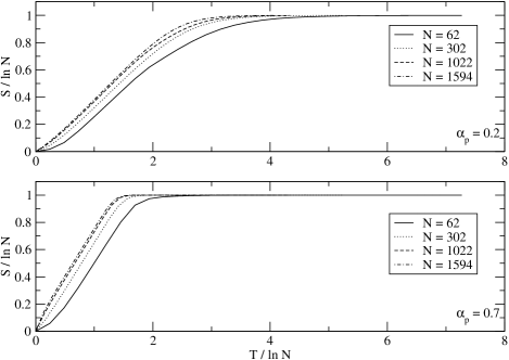
FIG. 6.: Scaling of the linear entropy growth with dimension of the Hilbert space of the system with diffusion on the momentum axis. The strength of the diffusion is kept constant by smoothing over a constant fraction of the system’s phase space. In relationship with Figures 5 and 6 both axis have been rescaled by $\log(N)$.

Our results show clearly that above some threshold for $\alpha$, the rate of entropy production is determined by the dynamics of the unitary quantum map, and in great measure by its classical counterpart). Why is this the case? We will argue here that it is possible to attribute the entropy production to two interconnected processes whose origin can be better explained by using a phase space representation for the quantum state. The reason is that in this way we can use some of the intuition we have about the behavior of the classical system. Consider an initial state that is represented by a localized and smooth phase space distribution (for concreteness we base our discussion on the Wigner function, see below). The application of the chaotic unitary map will distort the state in a way that, at least for short times (times smaller than $\log(N)$), will be consistent with the classical evolution. In a hyperbolic region this will mean that the initial wavepacket will be stretched along the unstable manifold and contracted along the stable one. In the case of the baker’s map (and only in this case) these two directions are the same all over phase space: the vertical direction -that we have called momentum - is stable (contracting) and the horizontal one - the coordinate - is unstable (expanding). The rate of expansion is equal to the Lyapunov exponent which in the baker’s map (and only in this case) is constant all over phase space and is equal to $\ln 2$. However, this expansion cannot proceed forever. As the phase space is finite, after some time the state will start experiencing the other essential feature of chaotic dynamics: folding. As soon as this process starts the quantum and classical evolutions will start deviating significantly from each other due to the quantum interference between the different folds. In the Wigner function (see below) these interferences appear as rapid oscillations with large negative values happening in between the folds and oscillating in directions parallel to them. These oscillations are the footprint of the quantum interference between the different pieces of the delocalized state.

The two interconnected effects generated by the diffusive map are: (a) the destruction of the interference fringes in the Wigner function, (b) the smoothing and widening of the regions where the Wigner function is already positive. It should be clear that the two effects have the same origin: diffusion, but it is worth distinguishing between them because they are effective for different types of states and can be analyzed separately under some special circumstances. In fact, process (a) affects states which have a quantum nature exhibiting important oscillations in the Wigner function. On the other hand, process (b) is present even for classical systems (in fact, in a classical difussive map process (b) is the only source of entropy). The important point is that even if we consider an initial state where only process (b) is important (i.e., a classical state), the dynamics of the system will create large scale quantum interference which will trigger process (a).

In the baker’s map the two processes can be analyzed separately. Thus, if we consider a non–unitary map producing diffusion only along the momentum (i.e., $\Delta x=0$ in (30)) only process (b) will be relevant. In fact, this is the case because an initial phase space distribution will tend to be contracted in the momentum direction while being expanded in the position direction. Folding will start to occur when the state reaches the boundary of the phase space. After that, quantum interference will develop between the different pieces of the packet and will be characterized by fringes which will be aligned along the vertical direction. Therefore, the fringes will not be significantly affected by diffusion. On the contrary, the effect of diffusion will be to fight against the contraction of the wavepacket along the momentum direction. One can see that diffusion will tend to compensate contraction and the Wigner function will tend to acquire a critical width along momentum. When this happens, the entropy will start growing at a rate fixed by the expansion rate which is the Lyapunov exponent. This is the scenario originally discussed in [3]: the entropy grows at the rate fixed by the Lyapunov exponent when the Wigner function reaches a critical width along the stable direction (contraction stops but expansion continues almost unafected by diffusion, therefore area grows exponentially which implies that entropy grows linearly).

The other extreme case is to consider a non–unitary map where difussion is along the position direction (i.e., $\Delta p=0$ in (30). In that case, diffusion will not prevent the system from contracting along the stable direction and therefore will not give rise to a critical width in that direction. However, entropy will still grow but it’s origin is entirely due to process (a). In fact. as soon as the phase space distribution starts to fold, interference fringes develop. These fringes are aligned along the momentum axis (since they correspond, roughly, to interference between two horizontal strips separated by a distance $1/2$). As the strips are macroscopically separated they will be very sensitive to diffusion along position. Thus, if the coupling strenght $\alpha$ is such that the fringes are washed out in just one iteration the mechanism will produce a mixture of two horizontal strips every iteration of the map producing one bit of entropy. The rate associated to this mechanism is the rate of folding that in the case of the baker’s map (and only in this case) is equal to the global Lyapunov exponent. Thus, the fact that both processes (a) and (b) give rise to the same rate is an accident of the baker’s map. In general the rate will not be the Lyapounov exponent but a combination of such exponent and the global folding rate. In any case, the general conclusion which is still valid is that the entropy production rate for classically chaotic systems will tend to be dominated by dynamical properties of the system becoming independent of the strength of the coupling to the environment.

It is interesting to present a simple analytic model to support the above discussion about entropy production. The simplest case is the one corresponding to process (b), where difussion is along the position direction. To simplify our model we will assume that the action of the baker’s map is just to transform a momentum eigenstate into a superposition of two such states:

$$\hat{B}|{k_{0}}\rangle=\frac{1}{\sqrt{2}}(|{\frac{k_{0}}{2}}\rangle+|{\frac{k_{0}+1}{2}}\rangle)$$ (33)

(this is a rough approximation for the baker’s map that neglects diffraction effects and relative phases but that captures the essential folding mechanism of the baker’s action in the large $N$ limit and away from saturation ). In this approximation, the unitary evolution turns each momentum state into a coherent superposition of two momentum states separated by a macroscopic distance $N/2$. According to (31), the momentum diffusion leaves untouched the diagonal - incoherent - elements for the density matrix of this state while suppressing, in the large M limit, the off-diagonal parts by a factor

$$\frac{\langle{i}|\hat{\rho}^{\prime}|{i+N/2}\rangle}{\langle{i}|\hat{\rho}|{i+N/2}\rangle}\approx 1-\alpha$$ (34)

With these assumptions it is simple to obtain an equation for the entropy as a function of time. Thus, after $t$ iterations the density matrix has $2^{t+n-1}$ matrix elements with value $2^{-t}(1-\alpha)^{n}$, with $n$ ranging from $1$ to $t$. Using this, we showed that the linear entropy is

$$S(t)=t\ln 2-\ln\big{[}(1-\alpha)^{2}(1+(2(1-\alpha)^{2})^{t})-1\big{]}.$$ (35)

The second term in this equation corrects the slope in the small $\alpha$ regime. The transition is predicted at a critical value of $\alpha_{c}=1-2^{-1/2}\approx 0.3$. For $\alpha>\alpha_{c}$ the second term becomes intependent of $t$ and the slope saturates at $\dot{S}=\ln 2$. In the weak coupling regime , for $\alpha<\alpha_{c}$ the growth is still linear, but the slope depends on the coupling strenght and is given - for long times - by

$$\dot{S}=-2\ln(1-\alpha)$$ (36)

In this regime the slope of the entropy is then linear with $\alpha$ - and independent of the Lyapounov exponent of the map. All the predictions of this simple model are confirmed by the numerical calculations. In Figure (7) we display the behavior of the rate $\dot{S}$ as a function of the coupling strength $\alpha$ during the regime of linear growth. The agreement between the simple model and the exact numerical results is very good, describing both coupling regimes very accurately. To see the limitations of the model we plot in Figure (8 the same quantities, but taken at later times, closer to the point where the entropy saturates due to the finiteness of the model. Here the agreement deteriorates as the assumptions of the model break down.

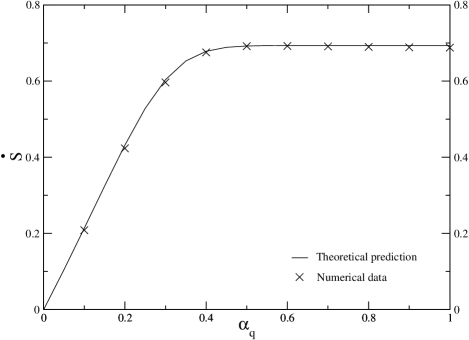
FIG. 7.: $\dot{S}_{2}$ vs. $\alpha$: Analytic prediction against numerical results. The analytic line and the numerical data points were not taken from the same iteration, in order to compensate for the fact that the initial state in the simulations was not a momentum eigenstate but a coherent state instead, which takes some iteratios to transform into something approximate to a momentum eigenstate.

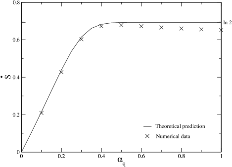
FIG. 8.: $\dot{S}_{2}$ vs. $\alpha$: Anaylitic prediction against numerical results some iterations after the ones depicted in graph 7

.

B Quantum classical correspondence. Wigner function

We also studied the evolution of the Wigner function for a variety of initial states both for the baker’s map and the Harper’s map. In Figures 10 and 11 we compare the classical (left), unitary (center) and quantum difussive (right) cases for these two maps. The general features that are observed are the following: The unitary map follows the classical evolution for up to a time which is of the order of $\log(N)$. After this time quantum interference develops between the different pieces of the Wigner function. These effects are responsible for the loss of correspondence between quantum and classical evolution that was discussed in [6, 28, 29, 30]. When the effect of the coupling to the environment is taken into account, it is clear that the correspondence between the quantum and the classical evolution is restored and holds for a much longer time. However, it is worth pointing out that the fact that our system is finite (i.e., it has $N$ orthogonal states) implies that saturation is achieved and the system approaches an equilibrium state. This equilibration takes place for times which are a few times $\log(N)$ as seen in the curves for the entropy (thus, as entropy grows linearly, it will approach the $\log(N)$ value relatively soon). Therefore, in this type of system the quantum classical correspondence is restored but has a rather short interesting dynamical regime. The nature of the final equilibrium state has footprints of the underlying classical dynamical system that are evident in the presence of decoherence. This is not so transparent by analyzing the final state for the Baker map but it is evident for the Harper’s map: the final state with decoherence is an equilibrium state where occuping uniformily all the available phase space with the remarkable exceptions of the regular islands.

By analyzing the Wigner distribution we can study the differences between the two processes contributing to the entropy growth that were discussed above. Thus, when difussion is along the direction of momentum it tends to prevent the contraction of the Wigner function but does not affect the interference fringes. On the other hand, when diffusion is along the position direction it does not affect the contraction but efficiently destroys the interference fringes. In Figure 9 we show a comparison of the Wigner function for the cases when diffusion is in position and momentum. It is clear that in the first case the width in momentum is significantly smaller than in the second while the interference fringes (that are alligned along momentum) are washed out much more efficiently. When the diffusion is along the stable manifold, the packet width does not shrink in momentum and approaches a critical width. Besides, the interference fringes are more noticeable. In the case of position diffusion there is also a critical width that in this case corresponds to the wavelength of the interference fringes that are no longer efficiently suppressed by diffusion (that damps all small wavelength fringes).

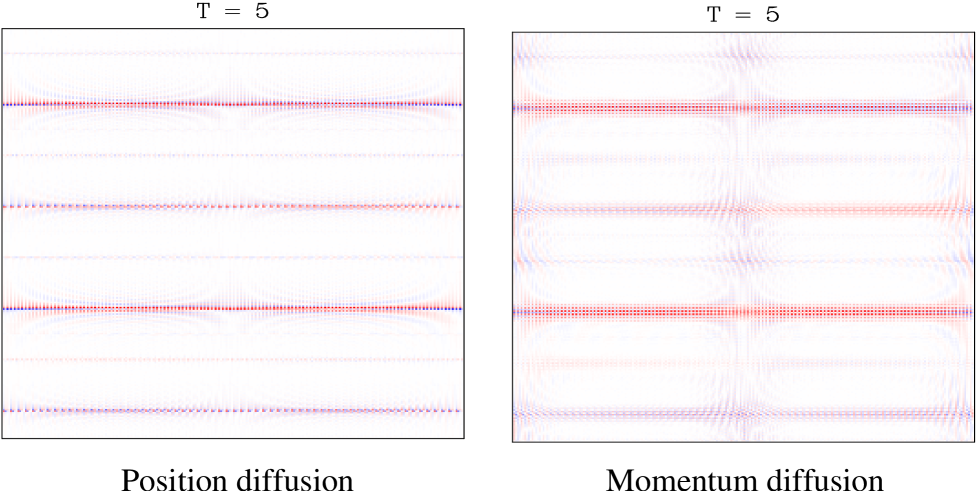
FIG. 9.: Comparison between diffusion in the different manifolds of the baker’s map.

V Conclusions

The main results in this paper come from numerical simulations of open quantum maps, particularly the baker’s and Harper’s map coupled to a diffusive environment. Our simulations provide strong numerical evidence supporting the conjecture put forward in [3]: when a quantum system whose classical analog is chaotic is subject to decoherence, there is a regime in which the rate of entropy production is determined by the system’s dynamical properties (Lyapunov exponents, folding rates, etc) and becomes independent of the strength of the coupling to the environment. Another interesting aspect of our results is the existence of a clear scaling for the entropy as a function of the dimensionality (or of the effective Planck constant). The scaled curves for the entropy become independent of $h=\frac{1}{N}$) with quantum corrections that decay as N grows. We also found cualitative evidence, looking at the phase space distributions, that the introduction of diffusion extends the time of coincidence between the classical and quantum evolutions. Our results also clarify the origin of entropy production allowing us to develop new intuitive explanations to understand the origin of the entropy growth (see [31] for another point of view based on the use of consistent histories). The two processes that are responsible for such growth (washing out of interference fringes and smoothing of the positive pieces of the Wigner function) can be studied separately only in the case of the baker’s map where stable and unstable manifolds have a global nature in phase space. The differences between the behavior of the entropy as a function of time for both non–unitary models (diffusion along position or along momentum) are illuminating: in both cases there is a regime in which the entropy grows linearly with a slope that is equal to the Lyapunov exponent (which is also the folding rate). The initial behavior is different in the two cases: when diffusion is along the position direction the entropy stays small initially until the wavepacket reaches the boundary of phase space and folding becomes effective. Then every iteration of the map creates new interference fringes that are rapidly destroyed by decoherence. Thus, the dominant process for entropy production is (a). When diffusion is along the momentum direction, entropy growth starts at early times. In this case the growth of entropy is produced by process (b) and is associated with the fact that diffusion tends to balance the effect of the contraction of the wavepacket along the stable direction giving rise to a critical width. In any case, our study shows that entropy growth at a rate fixed by the dynamics of the system rather than the coupling strength to the environment is, as first conjectured in [3] a characteristic of quantum chaos. The differences between this behavior and the one that characterizes integrable systems (or quantum states localized in stability islands like the ones present in Harper’s map) are quite dramatic (see [32] for related results).

This work was partially supported by grants from Ubacyt, Anpcyt, Conicet and Fundación Antorchas. JPP gratefully acknowledges the hospitality of ITP Santa Barbara where the final version of this manuscript was completed.

A Discrete Wigner function

We use a discrete version of the Wigner function, which we describe in more detail in [27]. Here we give the basic definitions to make the paper self–contained. The Wigner function is usually defined, for a continuous system, as

$$W(q,p)=\frac{1}{2\pi\hbar}\int_{-\infty}^{+\infty}\langle{q-\frac{y}{2}}|\hat{\rho}|{q+\frac{y}{2}}\rangle e^{i{\frac{p}{\hbar}y}}\,d{y}.$$ (A1)

This function is the expectation value of the so-called phase space point operators:

$$W(q,p)=\mathop{\operator@font tr}\nolimits(\hat{\rho}\hat{A}(q,p)).$$ (A2)

The operators $\hat{A}(q,p)$ have a number of interesting properties from which the properties of the Wigner function can be derived (in fact, they are hermitian operators, they form a complete basis, etc; see [27]). It turns out that in order to generalize all these properties to the discrete case it is necessary to use a phase space lattice of $2N\times 2N$ points and to define the phase space operators (in terms of the shift operators used in the body of the paper and defined in (7)) as

$$\hat{A}(q,p)=\frac{1}{2N}\hat{\cal U}^{q}\hat{R}\hat{\cal V}^{-p}\exp{i\pi qp/N}.$$ (A3)

Using these discrete phase space point operators the Wigner function has all the desired properties (it is real, it can be used to compute expectation values of operators and gives rise to all the correct marginal distributions when summed over any set of lines in the phase space grid). To explicitly compute this function one can use a variety of formulae among which we found convenient the following expression:

$$W(q_{j},p_{i}) = \frac{2}{N^{3/2}}e^{-i{\frac{2\pi}{N}(\frac{q_{j}p_{i}}{2}-2\chi_{p}\chi_{q})}}\times$$ (A5)

$$\sum_{n}\sum_{k}e^{i{\frac{2\pi}{N}(q_{j}k+p_{i}n)}}e^{-i{\frac{2\pi}{N}(n-\chi_{p})(k-\chi_{q})}}\langle{k}|\hat{\rho}|{n}\rangle$$

On the other hand, it takes a atraightforward calculation to show that the $\hat{A}(q,p)$ operators transform in the following way when subjected to translations (both in their continuous and discrete versions):

$$\hat{D}_{(\Delta q,\Delta p)}\hat{A}(q,p)\hat{D}^{\dagger}_{(\Delta q,\Delta p)}=\hat{A}(q+2\Delta q,p+2\Delta p)$$ (A6)

We can use this property and the definition of the Wigner function given in equation A2 to derive the equation 32 we use in the paper.

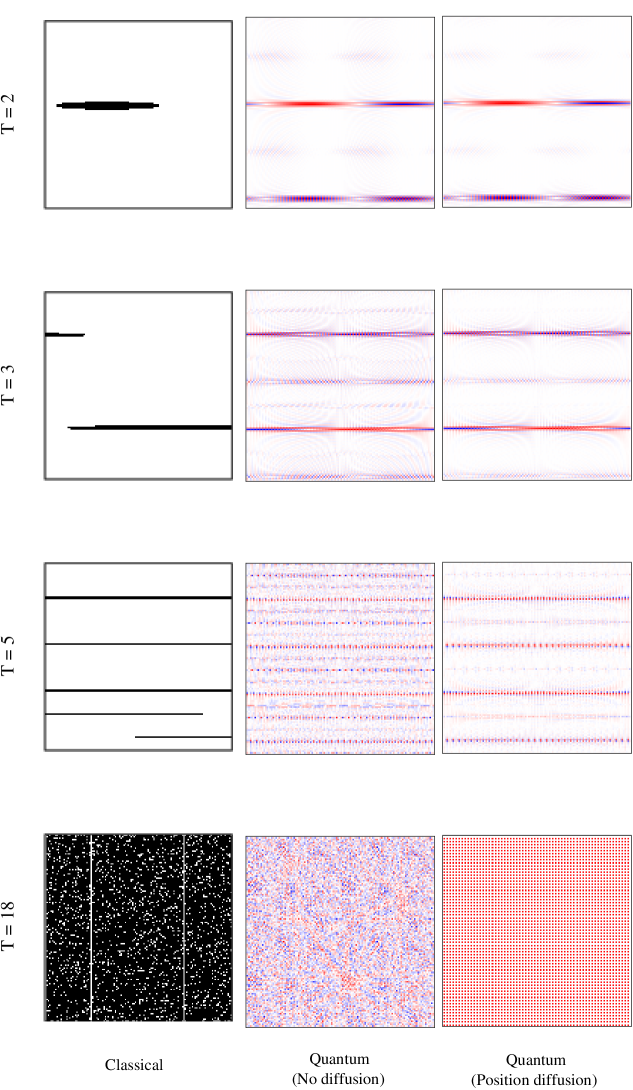
FIG. 10.: Phase space distribution at several steps in the evolution of the Baker map. The quantum versions have been computed with $N=62$.

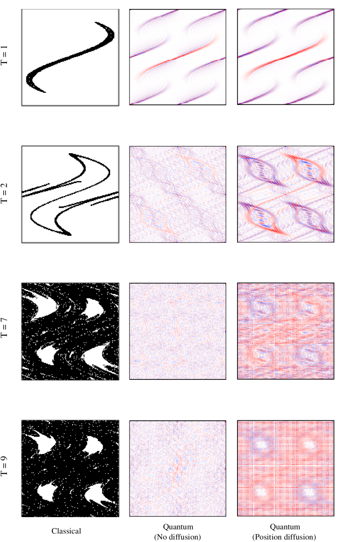
FIG. 11.: Phase space distribution at severals step in the evolution of the Harper’s map. The quantum version has diffusion parallel to the position axis and $N=62$, $\alpha_{q}=0.5$, $M=2$.

REFERENCES

- [1] W. H. Zurek, Physics Today 44, 36 (1991).
- [2] J. P. Paz and W. H. Zurek, (2001) Les Houches.
- [3] see J. P. Paz and W. H. Zurek, “Environment induced superselection and the transition from quantum to classical; (2001). in “Coherent matter waves, Les Houches Session LXXII;, edited by R Kaiser, C Westbrook and F David, EDP Sciences, Springer Verlag (Berlin) (2001) 533-614 and references therein. W. H. Zurek y J. P. Paz, Phys. Rev. Lett. 72 (1994) 2508; ibid. 75 (1995) 351.
- [4] Zurek, W. H. and Paz, J. P., Physica D83 (1995) 300.
- [5] D. Monteoliva and J. P. Paz, Phys. Rev. Lett. 87 (2000) 3373.
- [6] D. Monteoliva and J. P. Paz, Phys. Rev. E (2001) to appear (quant-ph/0105090).
- [7] Zurek, W. H., Physica Scripta T76 (1998) 186, also available at quant-ph/9802054.
- [8] Shiokawa, K., and Hu, B. L., Phys. Rev E 52 (1995) 2497.
- [9] Miller, P. A., and Sarkar, S. Phys. Rev. E 58, (1998) 4217; E 60 (1999) 1542.
- [10] A. K. Pattanayak, Phys. Rev. Lett. 83 (1999) 4526.
- [11] S. Nag, A. Lahiri and G. Ghosh, Entropy production due to coupling to a heat bath in the kicked rotor problem, quant-ph/0108099.
- [12] J. Schwinger, Proc. Nat. Acad, Sci.46 (1960), 570, 893.
- [13] V.I. Arnold and A. Avez, Ergodic Problems in Classical Mechanics, Benjamin, New York, (1968).
- [14] N.L. Balasz and A. Voros, Ann. Phys. 190 (1990) 1.
- [15] M. Saraceno, Ann. Phys. 199 (1990) 37.
- [16] A. Voros y M. Saraceno, Physica D79 (1994) 206.
- [17] R. Schack, Phys. Rev A57 (1998) 1634-1635; R. Schack and T. Brun, Phys. Rev. A 59 (1999) 2649-2658.
- [18] R. Schack and Caves C. M., Appl. Algebr. Eng. Comm. 10 (2000) 305-310; see also A. N. Soklakov and R. Schack, Phys. Rev. E 61 (2000) 5108-5114.
- [19] I. Chuang and M. Nielsen ”Quantum Information and Computation” (2000), Cambridge University Press.
- [20] F. Haake, Quantum signatures of chaos, Springer Series in Synergetics, edited by H. Haken, vol 54, Springer (Berlin, 1991).
- [21] P. Leboeuf, J. Kurchan, M.Feingold, D.Arovas, Phys.Rev.Lett 65 (1990) 3076.
- [22] B. Georgeot and D. L. Shepelyansky, Phys. Rev. Lett. 86 (2001) 2890-2893; B. Georgeot and D. L. Shepelyansky, Phys. Rev. Lett. 86 (2001) 5393-5396.
- [23] J. Preskill; Lecture Notes on Quantum Information and Computation available at www.theory.caltech.edu/people/preskill/ph229.
- [24] B. Schumacher, Phys. Rev. A 54 (1996) 2614.
- [25] H. Grabert, P. Shramm and G. L. Ingold, Phys. Rep. 168 (1998) 115; A. O. Caldeira and A. J. Leggett, Physica 121A (1983) 587-616; Phys. Rev. A 31 (1985) 1059; W. G. Unruh and W. H. Zurek, Phys. Rev. D 40 (1989) 1071-1094; F. Haake and R. Reibold, Phys.Rev, 32 (1985) 2462; B. L. Hu, J. P. Paz and Y. Zhang, Phys. Rev. Hu, B. L., Paz, J. P., and Zhang, Y., Phys. Rev. D 45 (1992) 2843; ibid D 47 (1993) 1576.
- [26] W. K. Wooters, Ann. Phys. NY 176 (1987), 1; A. Rivas, A. M. Ozorio de Almeida, Ann.Phys. 276 (1999), 123; A. Bouzouina, S. De Bievre, Comm. Math. Phys. 178 (1996) 83.
- [27] P. Bianucci, C. Miquel, J. P. Paz and M. Saraceno, Discrete Wigner functions and the phase space representation of quantum computers quant-ph/0105090; C. Miquel, J. P. Paz and M. Saraceno, Quantum computers in phase space in progress.
- [28] Berman, G. P., and Zaslavsky, G. M., Physica (Amsterdam) A91, 450 (1978).
- [29] Habib, S., Shizume, K., and Zurek, W. H., Phys. Rev. Lett, 80, 4361 (1998).
- [30] K. Inoue, M. Ohya, I.V. Volovich, On Quantum - Classical Correspondence for Baker’s Map, quant-ph/0108107.
- [31] A. N. Soklakov and R. Schack, Decoherence and linear entropy increase in the quantum baker’s map, quant-ph/0107071.
- [32] See, for example, recent studies of the behavior of fidelity–like quantities in condensed matter systems (attenuation of polarization echoes, etc): H. Pastawski, P. Levstein, G. Usaj, J. Raya and Hirschinger, Physica A 283 (2000) 166-170. The study of such quantities is relevant in connection to interesting experiments performed using NMR techniques; see H. Pastawski, G. Usaj, and P. Levstein, Chem. Phys. Lett. 261 329 (1996). For recent numerical work see: R. Jalabert and H. Pastawski Phys. Rev. Lett. 86 (2001) 2490-2493 and Ph. Jacquod, P.G. Silvestrov, C.W.J. Beenakker Golden rule decay versus Lyapunov decay of the quantum Loschmidt echo nlin.CD/0107044.