Quantum non ideal measurements

Abstract

We analyse non ideal quantum measurements described as scattering processes providing an estimator of the measured quantity. The sensitivity is expressed as an equivalent input noise. We address the Von Neumann problem of chained measurements and show the crucial role of preamplification.

I Introduction

Active systems are fundamental elements in high precision measurements in particular measurement on quantum systems. Amplifiers are used either for amplifying the signal to a macroscopic level or to make the system work around its optimal working point with the help of feedback loops. The analysis of sensitivity limits in these devices rises many questions related to fundamental processes as well as experimental constraints. How does the active feedback act on the quantum system? How does the coupling with the environment influence the sensitivity of the measurement? How are these process related to the fluctuation dissipation theorem? How do the experimental constraints interplay with the fundamental limitations of the sensitivity?

The aim of the present paper is to address the question of measurement on quantum systems with real measurement devices. We address this problem with quantum network theory. This approach provides a rigorous thermodynamical framework able to withstand the constraints of a quantum analysis of the measurement. In the same time, it makes possible a realistic description of real measurement devices.  Thermodynamic and quantum fluctuations are treated in the same footing. The measurement process is described as a scattering process allowing for a modular analysis of real quantum systems. Active systems such as the linear amplifier or the ideal operational amplifier are described in this framework. Here, the approach will be illustrated by analyzing the sensitivity of a cold damped capacitive accelerometer developed for fundamental physics applications in space [2, 3, 4].

We first present the analysis of a quantum measurement with a passive systems in term of quantum networks. Then, we use this approach to present the quantum analysis of measurements with an operational amplifier working in the ideal limit of infinite gain, infinite input impedance and null output impedance and we illustrate the theoretical framework with the example of a cold damped accelerometer. We conclude with an analysis of chained measurements

II Quantum Networks

The measurement of a physical quantity or signal corresponds to the obtention of a result or readout from a measureing device. In general, this is obtained after a few stages. Many times, the signal is transduced into an electrical signal which is amplified. After further processing, the resulting voltage drives a displaying or a storing device. The final result is thus obtained after a succession of stages.

As far as measurement at the quantum level is concerned, the principle is the same: a chain of processes leads from the quantum system to the readout of the meter. As a first insight into a quantum analysis of measurement, we will consider the detection of an electromagnetic wave with an antenna and first restrict our attention to the transduction of the wave into an electrical signal.

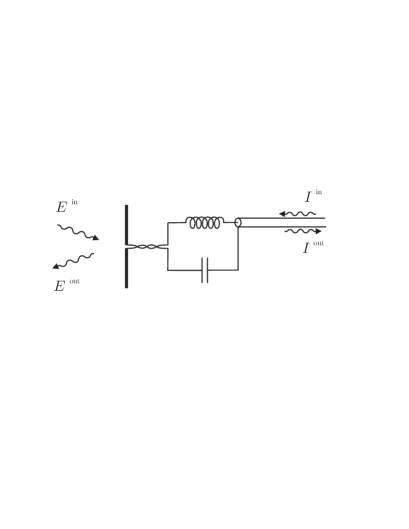
FIG. 1.: Model for the measurement of an electromagnetic field. An incoming electromagnetic wave $E^{\rm in}$ is detected by an antenna coupled to an electric resonator. The detection is provided by the current $I^{\rm out}$ leaving the coaxial line.The coupling of the measuring device with the environment by the antenna is also at the origin of dissipation due to the emission of a field $E^{\rm out}$. The coupling with the line is at the origin of current fluctuations $I^{\rm in}$ incoming by the line

As sketched on figure 1, a detecting antenna is coupled with an electrical resonator a coaxial line is used to extract an electrical signal from this system. The further steps as for instance amplification will be considered in the next section.

The the antenna is coupled to the electromagnetic field though one mode obtained as a linear combination of plane waves or spherical waves and corresponding to the radiation diagram of the antenna. In this mode two counterpropagating fields can be separated an incoming field $E^{{\rm in}}$ and an outgoing field $E^{{\rm out}}$. The incoming electromagnetic wave $E^{{\rm in}}$ puts into motion the electrons in the antenna and produces a current flow in the circuit. As a consequence of this current, a signal $I^{{\rm out}}$ with informations on the detected radiation is sent into the coaxial line. This electrical signal may then be used to feed a further element, for instance an amplifier. In addition, any incoming signal $I^{{\rm in}}$ arriving in the coaxial line also creates a current in the detector and can perturb the measurement. For example, if the line is at thermal equilibrium, it corresponds to the Johnson Nyquist noise. Finally, energy and information can be lost because of the emission of radiation by the antenna.

These phenomena, present in every measurement can be synthetized in the following way. In the frequency domain the output fields can be written as linear combinations of input fields. Throughout the paper, we will consider that a function $f$ is defined in the time domain (notation $f\left(t\right)$) or in the frequency domain (Kubo’s notation $f\left[\omega\right]$) and that these two representations are related trough the Fourier transform with the convention of quantum mechanics

$$f\left(t\right)=\int\frac{d\omega}{2\pi}f\left[\omega\right]e^{-i\omega t}$$ (1)

The electronics convention may be recovered by substituting $j$ to $-i$.

The detection and measurement is then described as a scattering process:

$$\left(\begin{array}[]{c}I^{{\rm out}}\\ E^{{\rm out}}\end{array}\right)=\left(\begin{array}[]{cc}\alpha&\beta\\ \gamma&\delta\end{array}\right)\left(\begin{array}[]{c}I^{{\rm in}}\\ E^{{\rm in}}\end{array}\right)$$ (2)

The measurement of the field $E^{{\rm in}}$ with the current $I^{{\rm out}}$ can be described with an estimator$\hat{E}^{{\rm in}}$

$$\hat{E}^{{\rm in}}=\frac{1}{\beta}I^{{\rm in}}=E^{{\rm in}}+\frac{\alpha}{\beta}I^{{\rm in}}$$ (3)

the incoming current fluctuations correspond to a noise in the measurement. It is also possible to express the output field $E^{{\rm out}}$

$$E^{{\rm out}}=\gamma I^{{\rm in}}+\delta E^{{\rm in}}$$ (4)

$\gamma I^{{\rm in}}$ coreponds to the back action noise on the measured device. This kind of description of a measurement can be generalized to more complex systems in the framework of quantum network theory.

In this approach, the role of the antenna and the line are to couple the measurement device with the outside world for inputs as well as for outputs. This coupling is associated to dissipation and fluctuations which are thus inavoidable in measurement processes. Dissipation corresponds to the loss of energy by the resonator as emitted radiation by the antenna or as an electrical signal by the line. Fluctuations corresponds to the detection of the thermal and quantum fluctuations of the input fields. Since Einstein and its study of the viscous damping of mechanical systems [5] the link between fluctuations and dissipation has been widely studied. For example with Johnson-Nyquist noise in resistive electrical elements [6]. In our situation, the energy loss of the oscillator has to be counterbalanced by the detection of thermal radiation by the antenna and the thermal current of the line. In the high temperature limit, it leads to the usual thermodynamic ${\frac{1}{2}}k_{B}T$ per degree of freedom, with $k_{B}$ being Boltzmann constant and $T$ the radiation temperature. Note that as a consequence, thermodynamics imposes constraints on the scatering matrix resulting from the two principles. We will analyse precisely these constraints in the general framework of quantum networks.

The classical result on the link between fluctuation and dissiaption was extended to take into account the quantum statistical properties of fluctuations[7, 8]. A general approach of these relations was widely studied in the framework of linear response theory [9, 10]. In particular, in the zero temperature limit, the detected field corresponds to the vacuum fluctuations of the electromagnetic field and the induced energy of the oscillator is the zero point energy ${\frac{1}{2}}\hbar\omega_{0}$, with $\omega_{0}$ the resonance frequency of the oscillator.

The elementary systems described up to now as well as more complex devices to be studied later in this paper may be described by using a systematic approach which may be termed as “quantum network theory”. Initially designed as a quantum extension of the classical theory of electrical networks [12], this theory was mainly developed through applications to optical systems [13, 14]. It has also been viewed as a generalized quantum extension of the linear response theory which is of interest for electrical systems as well [15]. It is fruitful for analyzing non-ideal quantum measurements containing active elements [16, 17].

In this quantum network approach, the various fluctuations entering the system, either by dissipative or by active elements, are described as input fields in a number of lines as depicted on 2.

For example, a resistance $R$ is modeled as a semi-infinite coaxial line $a$ with characteristic impedance $R$. In this line, current and voltage may be treated as quantum fields propagating in a two dimensional space-time.

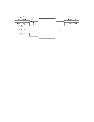
FIG. 2.: Representation of an electrical circuit as a quantum network. The central box is a reactive multipole which connects noise lines corresponding to the fluctuations entering the system, either by dissipative or by active elements. For example, the upper left port $n$ with voltage $U_{n}$ and current $I_{n}$ is connected to a line of impedance $R_{n}$ with inward and outward fields $a_{n}^{{\rm in}}$ and $a_{n}^{{\rm out}}$.

Free field operators $a^{{\rm in}}$ and $a^{{\rm out}}$ can be defined as the Fourier components of $I^{{\rm in}}$and $I^{{\rm out}}$ and related to the current and voltage at the end of the line:

$$I = \sqrt{\frac{\hbar\left|\omega\right|}{2}R}\left(a^{{\rm out}}-a^{{\rm in}}\right)$$ (5)

$$U = \sqrt{\frac{\hbar\left|\omega\right|}{2R}}\left(a^{{\rm out}}+a^{{\rm in}}\right)$$ (6)

They are normalized so that they obey the standard commutation relations

$$\left[a^{{\rm in}}\left[\omega\right],a^{{\rm in}}\left[\omega^{\prime}\right]\right] = \left[a^{{\rm out}}\left[\omega\right],a^{{\rm out}}\left[\omega^{\prime}\right]\right]$$ (7)

$$= 2\pi\ \delta\left(\omega+\omega^{\prime}\right)\ \varepsilon\left(\omega\right)$$ (8)

where $\varepsilon\left(\omega\right)$ denotes the sign of the frequency $\omega$. This relation just means that the positive and negative frequency components correspond respectively to the annihilation $a_{\omega}$ and creation $a_{\omega}^{\dagger}$ operators of quantum field theory

$$a^{{\rm in}}\left[\omega\right]=a_{\omega}\theta\left(\omega\right)+a_{-\omega}^{\dagger}\theta\left(-\omega\right)$$ (9)

$\theta\left(\omega\right)$ denotes the Heavyside function. Similarly, mechanical fluctuations as well as electromagnetical fluctuations can be expressed in term of these normalized fields.

To characterize the fluctuations of these noncommuting operators, we use the correlation function defined as the average value of the symmetrized product. With stationary noise, the correlation function depends only on the time difference

$$\left\langle a^{{\rm in}}\left(t\right)\cdot a^{{\rm in}}\left(t^{\prime}\right)\right\rangle = \sigma_{aa}^{{\rm in}}\left(t-t^{\prime}\right)$$ (10)

$$\left\langle a^{{\rm in}}\left[\omega\right]\cdot a^{{\rm in}}\left[\omega^{\prime}\right]\right\rangle = 2\pi\ \delta\left(\omega+\omega^{\prime}\right)\ \sigma_{aa}^{{\rm in}}\left[\omega\right]$$ (11)

The dot symbol denotes a symmetrized product for quantum operators.

In the case of a thermal bath, the noise spectrum is

$$\sigma_{aa}^{{\rm in}}\left[\omega\right]=\frac{1}{\exp\frac{\hbar\left|\omega\right|}{k_{B}T_{a}}-1}+\frac{1}{2}=\frac{1}{2}\coth\frac{\hbar\left|\omega\right|}{2k_{B}T_{a}}$$ (12)

One recognizes the black body spectrum or the number of bosons per mode for a field at temperature $T_{a}$ and a term $\frac{1}{2}$ corresponding to the quantum fluctuations. The energy per mode will be denoted in the following as an effective temperature $\Theta_{a}$

$$k_{B}\Theta_{a}=\hbar\left|\omega\right|\sigma_{aa}^{{\rm in}}\left[\omega\right]=\frac{\hbar\left|\omega\right|}{2}\coth\frac{\hbar\left|\omega\right|}{2k_{B}T_{a}}$$ (13)

In the high temperature limit the classical energy for an harmonic field of $k_{B}T_{a}$ per mode is recovered. In the low temperature limit, the energy $\frac{\hbar\left|\omega\right|}{2}$ corresponding to the ground state of a quantum harmonic oscillator is obtained. Note that the term $\frac{1}{2}$ corresponding to the zero point quantum fluctuations was added by Planck so that the difference with the classical result $k_{B}T_{a}$ tends to zero in the high temperature limit [11].

These results are easily translated to obtain the expression of the Johnson Nyquist noise power

$$\sigma_{U_{n}U_{n}}\left[\omega\right]=2R\hbar\left|\omega\right|\sigma_{aa}^{{\rm in}}\left[\omega\right]=2Rk_{B}\Theta_{a}$$ (14)

Our symmetric definition of the noise power spectrum leads to a factor $2$ difference with the electronic convention where only positive frequencies are considered.

The fields entering and leaving the network can be represented with column vectors ${\bf a}^{{\rm in}},{\bf a}^{{\rm out}}$ with components $a_{n}^{{\rm in}},$and $a_{n}^{{\rm out}}$ Input fields corresponding to different lines commute with each other. For simplicity, we also consider that the fields entering through the various ports are uncorrelated with each other.

The whole network is then associated with a scattering ${\bf S}$ matrix, also called repartition matrix [18], describing the transformation from the input fields to the output ones

$${\bf a}^{{\rm out}}={\bf S\ a}^{{\rm in}}$$ (15)

The output fields $a^{{\rm out}}$ are also free fields which obey the same commutation relations 8 as the input ones. In other words, ${\bf S}$ matrix is unitary. More generally, the unitarity of the ${\bf S}$ matrix is required to ensure the quantum consistency of the description. In the following section, we will make use of this property to deduce general properties of amplifiers. For passive systems the unitarity of ${\bf S}$ matrix ensures as well the verification of the two principles of thermodynamics. However, this unitarity is also valid in the presence of amplificating device.

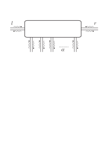
FIG. 3.: Quantum measurement as scattering by a network. The input signal $l^{in}$ enters the measurement device. An estimator is provided by the outgoing field $r^{out}$. The other lines $\alpha$ correspond to the various active and passive elements in the measureing device.

For the analysis of the measurement, two fields can be isolated, the input signal $l^{{\rm in}}$ and the output detection field $r^{{\rm out}}.$ The detection corresponds to figure 3. The detection is performed with the output detection signal $r^{{\rm out}}$. It is a linear combination of the incoming signal $l^{{\rm in}}$ and of input fields in the various noise lines. We normalize this expression so that the coefficient of proportionality appearing in front of the incoming signal $l^{{\rm in}}$ is reduced to unity. With this normalization, we obtain an estimator $\widehat{l}^{{\rm in}}$ which is just the sum of the true signal $l^{{\rm in}}$ to be measured and of an equivalent input noise:

$$\widehat{l}^{{\rm in}}=l^{{\rm in}}+\sum_{\alpha}\mu_{\alpha}\alpha^{{\rm in}}$$ (16)

where $\alpha^{{\rm in}}$ denote the various input fields corresponding to the active and passive elements in the detection device. The added noise spectrum $\Sigma_{ll}$ is obtained as

$$\Sigma_{ll}=\sum_{\alpha}\left|\mu_{\alpha}\right|^{2}\sigma_{\alpha\alpha}^{{\rm in}}$$ (17)

Within this approach, the succession of the different sages of the measurement are studied by using the output field of one stage as the input field of the next one.

III Measurement with active systems

We consider in this section the amplifying stage of the measurement. Quantum noise associated with linear amplifiers has been the subject of numerous works. In the line of thought initiated by early works on fluctuation-dissipation relations, active systems have been studied in the optical domain when maser and laser amplifiers were developed [19, 20, 21]. General thermodynamical constraints impose the existence of fluctuations for amplification as well as dissipation processes. The added noise determines the ultimate performance of linear amplifiers [22, 23] and plays a key role in the question of optimal information transfer in optical communication systems [24, 25].

Most practical applications of amplifiers in measurements involve ideal operational amplifiers operating in the limits of infinite gain, infinite input impedance and null output impedance. In order to deal with the pathologies that could arise in such a system, we consider that it operates with a feedback loop which fixes its effective gain and effective impedances [26].

In the framework of quantum networks, the noise sources of the amplifier can be modelled with two lines $a$ and $a^{\prime}$.

As depicted on figure 4, by coupling two coaxial lines denoted $l$ and $r$ respectively on the left port and the right port of the amplifier, one realizes a model of amplifying stage. The left line comes from a transducer so that the inward field $l^{{\rm in}}$ plays the role of the signal to be measured. Meanwhile, the right line goes to an electrical meter so that the outward field $r^{{\rm out}}$ plays the role of the meter readout. In connection with the discussions of Quantum Non Demolition measurements [27, 28], $l^{{\rm out}}$ appears as the back-action field sent back to the monitored system and $r^{{\rm in}}$ represents the fluctuations coming from the readout line. A reactive impedance $Z_{f}$ acts as feedback for the amplifier.

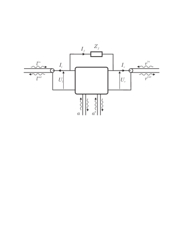
FIG. 4.: Measurement of an electrical signal $l^{{\rm in}}$ with an ideal operational amplifier working in the limit of infinite gain with a reactive feedback $Z_{f}$. The left (input) port $l$ correspond to the measured system and the a right (output) port $r$ provides the detection signal $r^{{\rm out}}$. The noise sources of the amplifier are modeled as input fields in the two noise lines $a$ and $a^{\prime}$

We now present the electrical equations associated with this measurement device. We first write the characteristic relations between the voltages and currents

$$U = U_{l}=U_{r}+Z_{f}I_{f}$$ (18)

$$I = I_{l}+I_{f}$$ (19)

Here, $U_{p}$ and $I_{p}$ are the voltage and current at the port $p$, i.e. at the end of the line $p=l$ or $r$, while $U$ and $I$ are the voltage and current noise generators associated with the operational amplifier itself (see Fig.1). $Z_{f}$ is the impedance feedback. All equations are implicitly written in the frequency representation and the impedances are functions of frequency. Equations (19) take a simple form because of the limits of infinite gain, infinite input impedance and null output impedance assumed for the ideal operational amplifier. We also suppose that the fields incoming through the various ports are uncorrelated with each other as well as with amplifier noises.

To obtain compact equations as well as for physical interpretations, we introduce here a voltage noise $U$ and a current noise $I$ as linear combination of the fields $a^{{\rm in}}$ and $a^{\prime{\rm in}}$.

$$U\left[\omega\right] = \sqrt{2\hbar\left|\omega\right|R_{a}}\left(a^{{\rm in}}\left[\omega\right]-a^{\prime{\rm in}}\left[-\omega\right]\right)$$ (20)

$$I\left[\omega\right] = \sqrt{\frac{2\hbar\left|\omega\right|}{R_{a}}}\left(a^{{\rm in}}\left[\omega\right]+a^{\prime{\rm in}}\left[-\omega\right]\right)$$ (21)

Note the presence of a conjugated field $a^{\prime{\rm in}}\left[-\omega\right]=a^{\prime{\rm in}}\left[\omega\right]^{\dagger}$ associated to the amplification process. In the following, the conjugation of $a^{\prime}$ will be assumed.

The parameter $R_{a}$ is determined by the ratio between voltage and current noise spectra of the amplifier

$$R_{a}=\sqrt{\frac{\sigma_{UU}}{\sigma_{II}}}$$ (22)

We can deduce from (21) that the voltage and current fluctuations $U$ and $I$ obey the following commutation relations

$$\left[U\left[\omega\right],U\left[\omega^{\prime}\right]\right] = \left[I\left[\omega\right],I\left[\omega^{\prime}\right]\right]=0$$ (23)

$$\left[U\left[\omega\right],I\left[\omega^{\prime}\right]\right] = 2\pi\ \hbar\omega\ \delta\left(\omega+\omega^{\prime}\right)$$ (24)

Hence, voltage and current fluctuations verify Heisenberg inequalities which determine the ultimate performance of the ideal operational amplifier used as a measurement device [26].

The fields $a^{{\rm in}}$ and $a^{\prime{\rm in}}$ are described by temperatures $T_{a}$ and $T_{a^{\prime}}$. We have assumed that these fluctuations are the same for all field quadratures, i.e. that the amplifier noises are phase-insensitive. Although this assumption is not mandatory for the forthcoming analysis, we also consider for simplicity that the specific impedance $R_{a}$ is constant over the spectral domain of interest.

We use the characteristic equations (19,6,21) associated with the amplifier and the lines to write the output fields $l^{{\rm out}}$ and $r^{{\rm out}}$ in terms of input fields $l^{{\rm in}}$, $r^{{\rm in}}$ and of amplifier noise sources $U$ and $I$

$$l^{{\rm out}} = -l^{{\rm in}}+\sqrt{\frac{2}{\hbar\left|\omega\right|R_{l}}}U$$ (25)

$$r^{{\rm out}} = -r^{{\rm in}}-2\frac{Z_{f}}{\sqrt{R_{r}R_{l}}}l^{{\rm in}}$$ (27)

$$+\sqrt{\frac{2}{\hbar\left|\omega\right|R_{r}}}\left(\frac{R_{l}+Z_{f}}{R_{l}}U-Z_{f}I\right)$$

The unitarity of the input output relations for $l^{{\rm out}}$ and $r^{{\rm out}}$ is ensured by the non commutation of the current and voltage noises.

In order to characterize the performance of the measurement device in terms of added noise, we introduce the estimator $\widehat{l}^{{\rm in}}$ of the signal $l^{{\rm in}}$ as it may be deduced from the knowledge of the meter readout $r^{{\rm out}}$

$$\widehat{l}^{{\rm in}} = -\frac{\sqrt{R_{r}R_{l}}}{2Z_{f}}r^{{\rm out}}$$ (28)

$$= l^{{\rm in}}+\frac{\sqrt{R_{l}R_{r}}}{2Z_{f}}r^{{\rm in}}-\left(\frac{1}{Z_{f}}+\frac{1}{R_{l}}-\frac{1}{R_{0}}\right)\frac{\sqrt{R_{l}R_{0}}}{2}a^{{\rm in}}$$ (30)

$$+\left(\frac{1}{Z_{f}}+\frac{1}{R_{l}}+\frac{1}{R_{0}}\right)\frac{\sqrt{R_{l}R_{0}}}{2}a^{\prime{\rm in}}$$

The estimator $\widehat{l}^{{\rm in}}$ would be identical to the measured signal $l^{{\rm in}}$ in the absence of added fluctuations. Hence the noise added by the measurement device is described by the supplementary terms assigned respectively to the Nyquist noise $r^{{\rm in}}$ in the readout as well as Nyquist noises $a^{{\rm in}}$ and $a^{\prime{\rm in}}$ in the two lines representing amplification noises. Notice that proper fluctuations of $l^{{\rm in}}$ are included in the signal and not in the added noise.

The whole added noise is characterized by a spectrum obtained as a sum of the uncorrelated noise spectra associated with these Nyquist noises

$$\Sigma = \frac{R_{l}R_{r}}{4\left|Z_{f}\right|^{2}}\sigma_{rr}^{{\rm in}}+\frac{R_{l}R_{0}}{4}\left|\frac{1}{Z_{f}}+\frac{1}{R_{l}}-\frac{1}{R_{0}}\right|^{2}\sigma_{aa}^{{\rm in}}$$ (32)

$$+\frac{R_{l}R_{0}}{4}\left|\frac{1}{Z_{f}}+\frac{1}{R_{l}}+\frac{1}{R_{0}}\right|^{2}\sigma_{a^{\prime}a^{\prime}}^{{\rm in}}$$

The Nyquist spectra are given by thermal equilibrium relations (14) with temperatures $\Theta_{r}$, $\Theta_{f}$, $\Theta_{a}$. The optimal sensitivity is obtained by matching the amplifier noise impedance $R_{0}$ with the impedance of the left line$R_{l}$.

We rewrite (30,32) under the simple forms

$$\widehat{l}^{{\rm in}} = \frac{1}{G}r^{{\rm out}}=l^{{\rm in}}+a^{\prime{\rm in}}-\frac{1}{G}\left(r^{{\rm in}}-a^{{\rm in}}+a^{\prime{\rm in}}\right)$$ (33)

$$G = -\frac{2Z_{f}}{\sqrt{R_{r}R_{l}}}$$ (34)

$G$ corresponds to the gain of the amplification for the normalized fields. In the limit of very lare gain the added noise reads:

$$\widehat{l}^{{\rm in}} = l^{{\rm in}}+a^{\prime{\rm in}}$$ (35)

$$\Sigma = \sigma_{a^{\prime}a^{\prime}}^{{\rm in}}$$ (36)

Finally this added noise is still decreased by going to a temperature $T_{b}$ as low as possible. At the limit of a null temperature, we recover the optimum of $3\,{\rm dB}$ added noise which is the same as for phase-insensitive linear amplifiers [25].

It is also possible analyse the succession of two amplifications

$r^{{\rm out}}$ is itself a quantum field it can be send at the iput of tan other amplifier as a field $l^{{}^{\prime}{\rm in}}=r^{{\rm out}}\$and can be measured in a similar manner with a quantum operational amplifier leading to an estimator

$$\hat{r}^{{\rm out}}=r^{{\rm out}}+b^{\prime{\rm in}}-\frac{1}{G^{\prime}}\left(r^{\prime{\rm in}}-b^{\prime{\rm in}}+b^{{\rm in}}\right)$$ (37)

Where the quantitities $b^{{\rm in}},b^{\prime{\rm in}},r^{\prime{\rm in}}$ and $G^{\prime}$ correspond to the second detection. As far as $r^{{\rm out}}$ is concerned, this is equivalet to a single detection. However, if we consider the estimator $\widehat{l}^{{\rm in}}$ for the two successive amplification of the signal $l^{{\rm in}}$ one obtains: is concerned, the added noise is negligeable thanks to the large amplification of the first detection. As a consequence, as soon as only the information on the first system $l^{{\rm in}}$ is concerned, the second detection can be considered as noiseless. In these condition the result $r^{{\rm out}}$ of the first measurement can be considered as a classical quantity in the further stage of the signal processing.

$$\widehat{l}^{{\rm in}} = l^{{\rm in}}+a^{\prime{\rm in}}-\frac{1}{G}\left(r^{{\rm in}}-a^{{\rm in}}+a^{\prime{\rm in}}+b^{\prime{\rm in}}\right)$$ (39)

$$+\frac{1}{GG\prime}\left(r^{\prime{\rm in}}-b^{\prime{\rm in}}+b^{{\rm in}}\right)$$

As aconsequence, with a large gain of the first amplification the only important noise source is $a^{\prime{\rm in}}.$

IV Analysis of a real device: the cold damped accelerometer

We come to the discussion of the ultimate performance of the cold damped capacitive accelerometer designed for fundamental physics experiments in space [17].

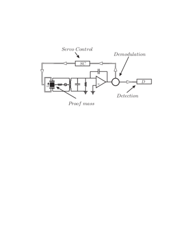
FIG. 5.: Scheme of the capacitive sensor. The proof mass is placed between two electrodes formed by the inner walls of the accelerometer cage. The position dependent capacitances are polarized by an AC sinewave source which induces a mean current at frequency $\omega_{t}$ in the symmetrical mode. The mass displacement is read as the current induced in the antisymmetric mode. An additional capacitance is inserted to make the antisymmetric mode resonant with $\omega_{t}$. The signal is detected after an ideal operational amplifier with capacitive feedback followed by a synchronous demodulation. The impedance of the detection line plays the role of a further resistance $R_{r}$. The detected signal then feds the servo loop used to keep the mass centered with respect to the cage.

The central element of the capacitive accelerometer is a parallelepipedic proof mass placed inside a box. The walls of these box are electrodes distant from the mass off a hundred micrometers. The proof mass is kept at the center of the cage by an electrostatic suspension. Since a three dimensional electrostatic suspension is instable, it is necessary to use an active suspension.

In the cage reference frame, an acceleration is transformed in an inertial force acting on the proof mass. The force necessary to compensate this inertial force is measured. In fact, as in most ultrasensitive measurements, the detected signal is the error signal used to compensate the effect of the measured phenomenon.

The essential elements of the accelerometer are presented in figure 5. The proof mass and the cage form two condensators. Any mass motion unbalances the differential detection bridge and provides the error signal. In order to avoid low frequency electrical noise, the electrical circuit is polarized with an AC voltage with a frequency of a hundred kilohertz. After demodulation, this signal is used for detection and as an error signal for a servo control loop which allows to keep the mass centered in its cage.

Furthermore, the derivative of this signal provides a force proportional to the mass velocity and simulates a friction force. This active friction is called cold damping since it may be noiseless. More precisely, the effective temperature of the fluctuations of this active friction is much lower than the physical temperature of the device.

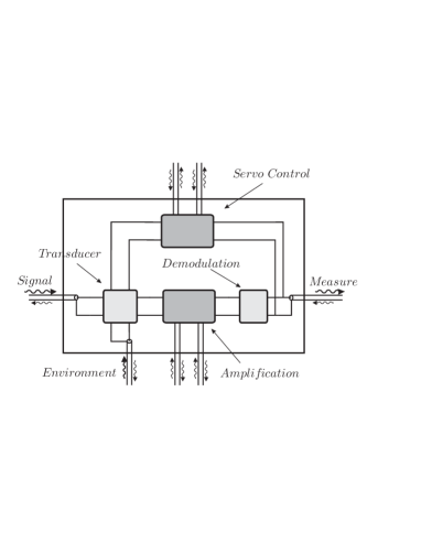
FIG. 6.: Scheme of the capacitive sensor represented as a quantum network. The essential elements of the network are represented. In particular, the input line, the mechanical dissipation corresponding to the coupling of the transducer with the environment, the detection amplifier with its two noise lines, the detection line and the feedback amplifier

The detection is performed with the output detection signal $r_{1}^{{\rm out}}$. It is a linear combination of the external force $F_{ext}$ and of input fields in the various noise lines. We normalize this expression so that the coefficient of proportionality appearing in front of the external force $F_{ext}$ is reduced to unity. With this normalization, we obtain a force estimator $\widehat{F}_{ext}$ which is just the sum of the true force $F_{ext}$ to be measured and of an equivalent input force noise. In the absence of feedback, the force estimator reads [17]:

$$\widehat{F}_{ext}=F_{ext}+\sum_{\alpha}\mu_{\alpha}\alpha^{{\rm in}}$$ (40)

where $\alpha^{{\rm in}}$ denote the various input fields corresponding to the active and passive elements in the accelerometer.

When the feedback is active, the servo loop efficiently maintains the mass at its equilibrium position and the velocity is no longer affected by the external force $F_{ext}$. The residual motion is interpreted as the difference between the real velocity of the mass and the velocity measured by the sensor. This means that the servo loop efficiently corrects the motion of the mass except for the sensing error. However the sensitivity to external force is still present in the correction signal. Quite remarkably, in the limit of an infinite loop gain and with the same approximations as above, the expression of the force estimator $\widehat{F}_{ext}$ is the same as in the free case [17].

The added noise spectrum $\Sigma_{FF}$ is obtained as

$$\Sigma_{FF}=\sum_{\alpha}\left|\mu_{\alpha}\right|^{2}\sigma_{\alpha\alpha}^{{\rm in}}$$ (41)

We have evaluated the whole noise spectrum $\Sigma_{FF}$ for the specific case of the instrument proposed for the $\mu$SCOPE space mission devoted to the test of the equivalence principle. Some of the main parameters of this system are listed below

$$M=0.27{\rm\ kg} H_{m}=1.3\times 10^{-5}{\rm\ kg\ s}^{-1}$$ (42)

$$\frac{\Omega}{2\pi}\simeq 5\times 10^{-4}{\rm\ Hz} \frac{\omega_{t}}{2\pi}\simeq 10^{5}{\rm\ Hz}$$ (43)

$$R_{a}=0.15\times 10^{6}\ \Omega \Theta_{a}=1.5{\rm\ K}$$ (44)

$M$ is the mass of the proof mass, $H_{m}$ is the residual mechanical damping force, $\frac{\Omega}{2\pi}$ is the frequency of the measured mechanical motion, $\frac{\omega_{t}}{2\pi}$ is the operating frequency of the electrical detection circuit. $R_{a}$ and $\Theta_{a}$ are the characteristic impedance and temperature of the amplifier.

In these conditions, the added noise spectrum is dominated by the mechanical Langevin forces

$$\Sigma_{FF} = 2H_{m}k_{B}\Theta_{m}$$ (45)

$$= 1.1\times 10^{-25}\left({\rm kg\ m\ s^{-2}}\right)^{2}/{\rm Hz}$$ (46)

This corresponds to a sensitivity in acceleration

$$\frac{\sqrt{\Sigma_{FF}}}{M}=1.2\times 10^{-12}{\rm\ m\ s^{-2}}/\sqrt{{\rm Hz}}$$ (47)

Taking into account the integration time of the experiment, this leads to the expected instrument performance corresponding to a test accuracy of $10^{-15}$.

In the present state-of-the-art instrument, the sensitivity is thus limited by the residual mechanical Langevin forces. The latter are due to the damping processes in the gold wire used to keep the proof mass at zero voltage [4]. With such a configuration, the detection noise is not a limiting factor. This is a remarkable result in a situation where the effective damping induced through the servo loop is much more efficient than the passive mechanical damping. This confirms the considerable interest of the cold damping technique for high sensitivity measurement devices.

Future fundamental physics missions in space will require even better sensitivities. To this aim, the wire will be removed and the charge of the test mass will be controlled by other means, for example UV photoemission. The mechanical Langevin noise will no longer be a limitation so that the analysis of the ultimate detection noise will become crucial for the optimization of the instrument performance. This also means that the electromechanical design configuration will have to be reoptimized taking into account the various noise sources associated with detection [17].

V Conclusion

In this analysis of chained quantum measurements, the preamplification settles the Von Neumann problem of determining where the measurement result can be considered as classical.

Notice that in our analysis of the cold damped accelerometer, this fact is important to treat properly the feedback. The result of the measurement is used to act on the quantum system. This action is provided by a quantum signal, however, we have shown that the noise added in the active feedback loop is negligeable compared to the noise of the first stage.

REFERENCES

- [1]
- [2] A. Bernard and P. Touboul, The GRADIO accelerometer: design and development status, Proc. ESA-NASA Workshop on the Solid Earth Mission ARISTOTELES, Anacapri, Italy (1991).
- [3] P. Touboul et al., Continuation of the GRADIO accelerometer predevelopment, ONERA Final Report 51/6114PY, 62/6114PY ESTEC Contract (1992, 1993).
- [4] E. Willemenot, Pendule de torsion à suspension électrostatique, très hautes résolutions des accéléromètres spatiaux pour la physique fondamentale, Thèse de Doctorat de l’université Paris 11 (1997).
- [5] A. Einstein, Annalen der Physik 17 (1905) 549.
- [6] H. Nyquist, Phys. Rev. 32 (1928) 110.
- [7] H.B. Callen and T.A. Welton, Phys. Rev. 83 (1951) 34.
- [8] L. Landau and E.M. Lifshitz, “Course of Theoretical Physics: Statistical Physics Part 1” (Butterworth-Heinemann, 1980) ch. 12.
- [9] R. Kubo, Rep. Prog. Phys. 29 (1966) 255.
- [10] E.M. Lifshitz and L.P. Pitaevskii, “Landau and Lifshitz, Course of Theoretical Physics, Statistical Physics Part 2” (Butterworth-Heinemann, 1980) ch. VIII.
- [11] M. Planck M. 1900 Verh. Deutsch. Phys. Ges. 13 138 (1911); W. Nernst ibid. 18 83 (1916)
- [12] J. Meixner, J. Math. Phys. 4 (1963) 154.
- [13] B. Yurke and J.S. Denker, Phys. Rev. A 29 (1984) 1419.
- [14] C.W. Gardiner, IBM J. Res. Dev. 32 (1988) 127.
- [15] J-M. Courty and S. Reynaud, Phys. Rev. A 46 (1992) 2766.
- [16] F. Grassia, Fluctuations quantiques et thermiques dans les transducteurs électromécaniques, Thèse de Doctorat de l’Université Pierre et Marie Curie (1998).
- [17] F. Grassia, J-M. Courty, S. Reynaud and P. Touboul , Eur. Phys. J. D 8, 101, quant-ph/9904073
- [18] M. Feldmann, Théorie des réseaux et systèmes linéaires, (Eyrolles 1986)
- [19] H. Heffner, Proc IRE 50 (1962) 1604.
- [20] H.A. Haus and J.A. Mullen, Phys. Rev. 128 (1962) 2407.
- [21] J.P. Gordon, L.R. Walker and W.H. Louisell, Phys. Rev. 130 (1963) 806.
- [22] C.M. Caves, Phys. Rev. D26 (1982) 1817.
- [23] R. Loudon and T.J. Shephered, Optica Acta 31 (1984) 1243.
- [24] J.P. Gordon, Proc. IRE (1962) 1898.
- [25] H. Takahasi, in “Advances in Communication Systems” ed. A.V. Balakrishnan (Academic, 1965) 227.
- [26] J-M. Courty, F. Grassia and S. Reynaud, Europhys. Lett, 46 (1), pp. 31-37 (1999), quant-ph/9811062.
- [27] V.B. Braginsky and F.Ya. Khalili, “Quantum Measurement” (Cambridge University Press, 1992).
- [28] P. Grangier, J.M. Courty and S. Reynaud, Opt. Comm. 89 (1992) 99.