Decoherence of geometric phase gates

Abstract

We consider the effects of certain forms of decoherence applied to both adiabatic and non-adiabatic geometric phase quantum gates. For a single qubit we illustrate path-dependent sensitivity to anisotropic noise and for two qubits we quantify the loss of entanglement as a function of decoherence.

The discoveries of quantum algorithms for factorization shor1 and searching grov1 , and techniques for quantum error correction shor2 ; steane1 (and subsequent fault-tolerant methods) have generated considerable motivation for the realisation of quantum computing (QC) hardware. Significant progress has been made at the few qubit level; at present many possible alternative routes are under exploration fortschritte . The use of fundamental entities as qubits currently leads the way; however, there is growing longer term hope that fabricated condensed matter systems (maybe still using fundamental rather than fabricated qubits) may provide the vehicle for scalability in qubit number. Nevertheless, at present the decoherence problems in such systems loom very large indeed. Fault-tolerant techniques cannot be brought into play unless the underlying decoherence rates are small in the first place.

As arbitrary single-qubit gates and some entangling two-qubit gate are universal for quantum computing div1 ; lloyd1 ; barenco1 , experimental QC focuses on realising such gates. Whilst it would be unfair to deem single-qubit gates trivial, the entangling of qubits represents the first major hurdle—one cannot claim to have a serious QC candidate until this has been achieved. Nevertheless, with any new contender it is natural to investigate the simplest gates first, before progressing to those based on qubit coupling. Clearly a method for inferring the likely level of entanglement in a two-qubit gate from the results of single qubit experiments is a handy tool. This is the basis of the simulation approach we present here in the form of a specific example. It is certainly true that detailed calculations of decoherence effects (based on tracing over microscopic environments) can yield considerable understanding of the form of decoherence seen by a qubit, and can sometimes give estimates of decoherence rates; however, in any experimental realisation the ultimate calibration of decoherence is through measurement. Given this, we consider a simple simulation approach which, based on the observations of single qubit gates, enables estimation of the level of entanglement (if any!) that could be expected in a two-qubit gate with similar qubits. This relies on some advanced knowledge of the form of the dominant decohering mechanisms (although some of this may be inferred from various independent single-qubit experiments) and an assumption of environment effects in interacting two-qubit experiments being similar to those in the single-qubit experiments. If the former are worse, for example due to additional external source terms in the Hamiltonian, then an optimistic upper bound on entanglement results. Despite these constraints, the simulation approach could be very useful for new experimental QC investigations.

To illustrate the approach, we apply it to geometric phase gates jones1 ; ekert1 ; falci1 . This provides an example of the approach; however, the specific case of geometric phase gates is of interest in its own right, since the technique has already been applied to NMR experiments jones1 , has been proposed for use with superconducting qubits falci1 and, in principle, can be applied to other realisations of qubits with suitable source terms in their Hamiltonians. We quantify the effects of different forms of decoherence applied to single qubit phase gates, and the loss of entanglement for a conditional two-qubit gate. The same approach can also be applied to all forms of dynamically generated gates; a broader detailed study will be presented in a future paper.

The model of decoherence we use is Markovian, with the reduced density operator $\rho$ of the qubit system described by a Bloch-type master equation

$$\dot{\rho}=-i\left[H,\rho\right]+\sum_{m}\left(L_{m}\rho L_{m}^{\dagger}-\frac{1}{2}L_{m}^{\dagger}L_{m}\rho-\frac{1}{2}\rho L_{m}^{\dagger}L_{m}\right)\;,$$ (1)

where $H$ is the system Hamiltonian, the operators $\{L_{m}\}$ represent the coupling to the environment and $\hbar=1$. The implicit origin of the non-unitary evolution generated by the $\{L_{m}\}$ is coupling to a bath of environment degrees of freedom, which are traced out to give the reduced $\rho$. The form of Eq.(1) is somewhat restrictive, but within this Markovian limit it is possible to describe phenomena such as dissipation (spontaneous decay and finite temperature stimulated effects), white noise Hamiltonian terms and quantum measurement interactions. It is therefore possible to treat a number of realistic forms of decoherence. The master equation (1) can be solved in many simple cases; however, in order to be able to treat the types of time dependent Hamiltonians (including pulses etc.) used for the realisation of actual quantum gates, we generally work numerically. We use a quantum trajectory method, quantum state diffusion perc1 ; schack1 ; schack2 , to solve the master equation (1) through averages over stochastically evolving quantum states. Whilst we only give statistical data here, it is worth noting that (ensemble NMR systems aside) since actual quantum gates/computations run on individual systems, such simulation techniques in fact produce results in a manner very akin to actual QC experiments and examination of individual trajectories can provide additional insight perc1 . In all examples presented here the averages are over 1000 trajectories unless otherwise stated.

Our first example is a single qubit geometric phase gate. In order to generate a purely geometric phase, the dynamical phases acquired by the different amplitudes in an arbitrary qubit state have to be cancelled ekert1 ; falci1 . We use the scenario of Ref.10. The path traversed in parameter space is amenable to the investigation of different forms of decoherence and it has also been implemented experimentally jones1 . A spin qubit ($|\uparrow_{z}\rangle\equiv|0\rangle$ , $|\downarrow_{z}\rangle\equiv|1\rangle$) is subject to a static $z$-magnetic field $\omega_{0}$ and (within the usual rotating wave approximation) a field of amplitude $\omega_{1}$ and phase $\phi$ at angular frequency $\omega$. The general Hamiltonian is

$$H=\frac{\omega_{0}}{2}\sigma_{z}+\frac{\omega_{1}}{2}\left[\cos(\omega t+\phi)\sigma_{x}+\sin(\omega t+\phi)\sigma_{y}\right],$$ (2)

and to effect an ideal phase gate the spin is subjected to the unitary sequence $U_{4\gamma}=\Pi\,\bar{T}\,\bar{C}\,T\,\Pi\,\bar{T}\,C\,T$ . Here $T$ is a tipping of the magnetic field through angle $\theta$ (ramping $\omega_{1}$ from zero, with $\cos\theta=(\omega_{0}-\omega)/\sqrt{(\omega_{0}-\omega)^{2}+\omega_{1}^{2}}$ with $\phi$ at zero, $C$ is a $2\pi$ rotation of the phase $\phi$ at fixed $\omega_{1}$ and the bars denote the reversed paths. These operations have to be carried out adiabatically to avoid errors in the spin component amplitudes . Fast $\pi$-pulses $\Pi$ interchange the $\uparrow$ and $\downarrow$ amplitudes half way through and at the end (to cancel the dynamical phase contributions). The ideal gate to effect a relative phase of $\gamma_{B}=4\gamma$ on $|\psi\rangle\equiv 2^{-1/2}(|0\rangle+|1\rangle)$ is

$$U_{4\gamma}|\psi\rangle=2^{-1/2}(\exp(-2i\gamma)|0\rangle+\exp(2i\gamma)|1\rangle),$$ (3)

where $\gamma=\pi(1-\cos\theta)$ is the solid angle subtended by $C$ at the origin. Part of the appeal of this form of quantum gate is its potentially different sensitivities to different forms of decoherence; a potential drawback is the need for adiabaticity, so the gate is slow and decoherence has longer to bite.

We have studied these effects in detail. Results are shown in Fig. 1(a) for the effects of noise in the $x$- or $z$-components of the magnetic field, for two different $\gamma_{B}$. The gate was run adiabatically giving a zero decoherence fidelity of $f=0.999984$ for $\gamma_{B}=\pi$ and $f=0.999993$ for $\gamma_{B}=\pi/8$. For the smaller $\gamma_{B}$, which corresponds to a tipping of $14.3615\deg$ (so the instantaneous energy eigenstates remain closer to $\uparrow$ and $\downarrow$ in $z$), the system is clearly significantly more sensitive to $z$-noise compared to $x$-noise . On the other hand, for the larger $\gamma_{B}$ where the tipping is $41.4096\deg$ there is less distinction.

   

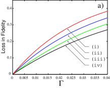
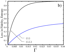
Figure 1: The effects of anisotropic noise (generated by $L=\kappa\sigma_{x}$ or $L=\kappa\sigma_{z}$) on the gate Eq.(3) are shown in a) for $\omega_{0}-\omega=100$. For adiabaticity $T$ takes (dimensionless) time $\pi$ and $C$ takes $2\pi$. The $\Pi$’s are square pulses taking time $\pi/100$. The ratio of these slow and fast operations is comparable to the frequency ratio in jones1 . The loss in fidelity $(1-f)$ is shown against the noise parameter $\Gamma=\kappa^{2}$: $\gamma_{B}=\pi/8$, $z$-noise (i) and $x$-noise (iv); $\gamma_{B}=\pi$, $z$-noise (ii) and $x$-noise (iii). In b) the effects of isotropic noise (generated by three independent $L_{i}=\kappa\sigma_{i}$ for $i=x,y,z$) on the gate Eq.(3) for $\gamma_{B}=\pi$. $(1-f)$ (i) and entropy $S=-Tr(\rho\log_{2}\rho)$ (ii) are shown against $\Gamma=\kappa^{2}$.

The case of isotropic noise is illustrated in Fig. 1(b). The small-$\Gamma$ rate of fidelity loss is twice that of the worst behaviour in Fig. 1(a) (which follows from a simple analytic estimate) and indeed the whole fidelity loss fits well with the analytic form $1-f=\frac{1}{2}(1-\exp(-4\Gamma\tau))$ where $\tau$ is the gate duration. Provided that the gate is adiabatic, the effects of isotropic noise are set by the gate length and level of decoherence, independent of the gate details. Also shown in Fig. 1(b) is the final system entropy as a function of $\Gamma$. For small $\Gamma$ the entropy (loss of information) increases significantly faster than the loss in fidelity.

Our second example is the more important case of a conditional two-qubit geometric gate ekert1 , where entanglement is generated, or not, depending upon the level of decoherence. This requires two spin qubits with bare transition frequencies of $\omega_{a}$ (target qubit) and $\omega_{b}$ (control qubit) and $\omega_{a}\gg\omega_{b}$. An interaction Hamiltonian of $H_{int}=\frac{J}{4}\sigma_{az}\sigma_{bz}$ generates the conditional phase. This form of interaction is that appropriate for NMR and certain condensed matter qubits. We have left $J$ fixed for the simulations presented here (as is appropriate for NMR systems), but in principle this coupling may be tunable for some condensed matter scenarios. A conditional phase gate (introducing $\Delta\gamma=\gamma_{B}(\uparrow_{b})-\gamma_{B}(\downarrow_{b})$, for the two states of the control) is realised by the unitary sequence $U_{\Delta\gamma}=\Pi^{b}U_{\gamma_{B}}^{a}\Pi^{b}U_{\gamma_{B}}^{a}$. Here superscripts refer to the qubit operated upon and $U_{\gamma_{B}}$ is the same as $U_{4\gamma}$ but with the final $\Pi$ removed. For $|\Psi\rangle_{ab}=|\psi\rangle_{a}|\psi\rangle_{b}$ this generates

$$U_{\Delta\gamma}|\Psi\rangle_{ab}=\frac{1}{2}\left(\exp(-2i\Delta\gamma)|0\rangle_{a}|0\rangle_{b}+\exp(2i\Delta\gamma)|0\rangle_{a}|1\rangle_{b}\right.$$

$$\left.+\exp(2i\Delta\gamma)|1\rangle_{a}|0\rangle_{b}+\exp(-2i\Delta\gamma)|1\rangle_{a}|1\rangle_{b}\right)\;.$$ (4)

For a phase of $\Delta\gamma=\frac{\pi}{8}$ this state has a concurrence conref of unity and so is a maximally entangled two-qubit state.

We have chosen the coupling and frequency parameters so that the zero decoherence state at the end of the simulated conditional phase gate is maximally entangled with fidelity of 0.999946, and then investigated this gate under various forms of decoherence. Examples of the results are shown in Fig. 2.

   

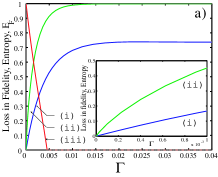
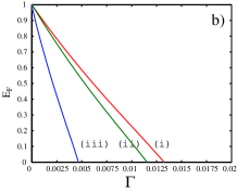
Figure 2: The effects of equal isotropic noise ($L_{i}=\kappa\sigma_{i}$ for $i=x,y,z$) applied to both qubits for the gate of Eq.(4) are displayed in a) with $\Delta\gamma=\frac{\pi}{8}$. Shown are plots of the loss in fidelity (i), the entropy $S=-Tr(\rho\log_{4}\rho)$ (ii) and the entanglement of formation (EOF) (iii) as a function of $\Gamma=\kappa^{2}$. The gate timings are as in Fig. 1 and additional parameters used are $\omega_{a}-\omega=100$, $\omega_{b}=1$, $\omega_{1}=87.9238$ and $J=37.5$. The entropy is base 4 to ensure a maximum value of 1. Also shown in a) is an enlargement of the region near $\Gamma=0$. In b) we also show the decrease in EOF as a function of $\Gamma$ for $s_{x}$ (i), $s_{z}$ (ii) and isotropic (iii) noise on each qubit.

Clearly the rate of fidelity loss and the sympathetic increase in entropy are correspondingly greater for this system as noise is acting independently on the two qubits. For this system $\rho$ was reconstructed by tomography tomogref from the sixteen expectation values $\langle\sigma_{ai}\sigma_{bj}\rangle$ for $i,j=0,x,y,z$ ($\sigma_{0}\equiv Identity$), akin to what is needed in any two-qubit experiment for a full reconstruction of $\rho$. From this it is possible to compute the entropy and some measure of entanglement. For illustration we use the entanglement of formation (EOF) eofref as this gives an upper bound on the level of decoherence for which some entanglement can be said to exist ($\Gamma_{thres}=0.00445$ for isotropic noise in our example).

The maximally entangling parameters used for Fig. 2 generate relatively large tipping angles, so there is only a slight sensitivity to the direction of anisotropic noise applied to both qubits, as shown in Fig. 2(b). Furthermore, detailed studies not illustrated here show that there is only a minor difference between the separate effects of noise on the control and the target, so from an experimental perspective on such a gate, there is nothing to be gained by singling out either of these for decoherence reduction measures (e.g. error correction). Both these points hold right down into the very small decoherence regime, where any practical system would have to operate.

In our simulations so far the gate times have been set to ensure adiabaticity. Such gates are relatively slow and therefore exposed to the ravages of decoherence for longer. Conventional dynamic gates can run much more quickly and so for comparison we investigate a dynamic gate based on the same interaction as the entangling adiabatic gate. The gate is realised by the unitary evolution $U(T)=\exp\left[i\frac{JT}{4}\sigma_{az}\sigma_{bz}\right]$ where we again choose $J=37.5$ and $T$ is now the interaction time. In the absence of decoherence this produces the maximally entangled state $|\Psi\rangle_{ab}=\frac{1}{2}e^{-i{\pi\over 4}}\left(|0\rangle_{a}|0\rangle_{b}+i|0\rangle_{a}|1\rangle_{b}+i|1\rangle_{a}|0\rangle_{b}+|1\rangle_{a}|1\rangle_{b}\right)$ with a fidelity of 1 if the gate acts for a total time $T_{tot}=2\pi/75$. For the adiabatic geometric phase gate $T_{tot}=12.0004\pi$, so the dynamic gate is approximately 450 times faster and its speed is limited directly by the strength of $J$. The results for this dynamic gate are illustrated in Fig. 3(a).

   

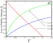
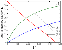
Figure 3: The effects of equal isotropic noise applied to both qubits for the dynamic gate are displayed in a) and to the nonadiabatic geometric gate in b). Shown in the plots are the loss in fidelity (i), the entropy $S=-Tr(\rho\log_{4}\rho)$ (ii) and the entanglement of formation (iii) as a function of $\Gamma$. For the dynamic gate the following parameters were chosen: $J=37.5$ and $T=\pi/J$. For the nonadiabatic fast geometric gate $J=37.5$, $\delta\omega=18.75$, $\omega_{B}=0.01$.

As isotropic noise acts on the dynamic gate, the entanglement of formation falls to zero at $\Gamma_{thres}\sim 2$ (compared with $\Gamma_{thres}=0.00445$ for the adiabatic gate). In fact we find that $\Gamma_{thres}\;T_{tot}\sim 4\pi/75$ for both the adiabatic geometric gate and the dynamic gate. Therefore, as the adiabatic gate operates for a significantly longer time, it is much more severely affected by decoherence. This has serious implications for the physical realisation of such a geometric gate. Recently, however, it has been proposed to use the non-adiabatic, or Aharonov-Anandan, phase to speed up geometric phase gates xbin1 . Here the achievable reduction in decoherence is not entirely clear as this technique also introduces new potential decoherence sources blais1 . We implement the unitary sequence $R_{x}^{a}(\pi/2)R_{z}^{a}(-\pi/2)\tilde{U}(\pi/4)R_{y}^{a}(-\pi/2)$ where $\tilde{U}(\pi/4)=R_{x}^{a}(3\pi/4)U(\pi/J)R_{x}^{a}(-\pi/2)U(\pi/J)R_{x}^{a}(-\pi/4)$ to produce the maximally entangled state $|\Psi\rangle_{ab}$. Here $R_{x}^{a}(\theta)$ indicates a rotation of $\theta$ about the $x$ axis. The results of isotropic noise acting on both qubits are displayed in Fig. 3(b). As this fast geometric gate has two periods of free evolution it acts for twice as long as the dynamic gate. Hence, it is subject to the effects of decoherence for longer and entanglement is again lost at a faster rate (slightly greater than twice the rate, $\Gamma_{thres}\sim 0.945$). Overall, our results suggest that geometric gates probably only offer a real advantage if they can be implemented faster than the equivalent dynamical gates. At present, such proposed gates do not beat the dynamic gate time ($\pi/J$ for our example), and it is not obvious that this is possible given both approaches realise entanglement through interacting qubit evolution. However, whether non-adiabatic geometric gates can be implemented more quickly is an open and critically important question currently under investigation.

A number of comments can be made in conclusion.
(1) Single qubit geometric phase gates can show some sensitivity to the direction of anisotropic noise, but this is path-dependent. In our example, if the path is chosen to generate a large ($\sim\pi$) relative phase between the qubit amplitudes, there is very little sensitivity.
(2) From the general perspective of our simulation approach, single qubit gate behaviour can be used with experimental results to calibrate the level of decoherence present in a system. Although the anisotropic noise-sensitive gates may be of limited use for actual quantum information processing (due to the small phase difference generated), they may be applied, for example coupled with the ability to reorientate the external static magnetic field ($z$-axis), in mapping out the forms of decoherence acting on a qubit, in addition to calibrating them. This could be extremely useful for new experimental systems where the dominant environmental coupling is unclear in advance.
(3) The single qubit decoherence calibrations can be used to predict the expected level of entanglement in two-qubit gates (as illustrated in Fig. 2) prior to experiment.
(4) The adiabatic gates discussed here are slow (relative to the timescale for dynamic gates) and so exposed to the ravages of decoherence for longer. To overcome this it is necessary to perform geometric gates faster than the equivalent dynamic gate. Whether they can be made faster than the dynamic gate is a unanswered question left for future investigation. The practical use of such geometric gates depends upon the resulting answer.

We thank Jonathan Jones, Andrew Briggs and Rüdiger Schack for helpful conversations and Richard Cardwell for technical assistance. Work supported in part by European Commission grant IST-1999-29110 MAGQIP.

References

- (1) P. W. Shor, p. 124 in Proceedings of the 35th Annual Symposium on the Foundations of Computer Science, ed. S. Goldwasser (IEEE Computer Society Press, Los Alamitos, CA, 1994); SIAM J. Computing 26, 1484 (1997); quant-ph/9508027.
- (2) L. K. Grover, p. 212 in Proceedings, 28th Annual ACM Symposium on the Theory of Computing (STOC), (May 1996); quant-ph/9605043.
- (3) P. W. Shor, Phys. Rev. A 52, 2493 (1995).
- (4) A. M. Steane, Phys. Rev. Lett. 77, 793 (1996); Proc. Roy. Soc. Lond. A 452, 2551 (1996).
- (5) A comprehensive (but by no means exhaustive) recent collection of papers (with citations to all the original references/proposals is: Fortschritte der Physik 48, No. 9-11 (2000), Special Focus Issue on “Experimental Proposals for Quantum Computation”.
- (6) D. P. DiVincenzo, Phys. Rev. A 51, 1015 (1995).
- (7) S. Lloyd, Phys. Rev. Lett. 75, 346 (1995).
- (8) A. Barenco, C. H. Bennett, R. Cleve, D. P. DiVincenzo, N. Margolis, T. Sleator, J. Smolin and H. Weinfurter, Phys. Rev. A 52, 3457 (1995).
- (9) J. A. Jones, V. Vedral, A. Ekert and G. Castagnoli, Nature 403, 869 (2000).
- (10) A. Ekert, M. Ericsson, P. Hayden, H. Inamori, J. A. Jones, D. K. L. Oi and V. Vedral, “Geometric Quantum Computation”, to appear in J. Mod. Opt., quant-ph/0004015.
- (11) G. Falci, R. Fazio, G. Massimo Palma, J. Siewert and V. Vedral, Nature 407, 355 (2000).
- (12) I. C. Percival, Quantum State Diffusion, (Cambridge University Press) and references therein.
- (13) R. Schack and T. A. Brun, Comp. Phys. Comm. 102, 210 (1997).
- (14) We have adapted the software of schack1 from http://www.ma.rhbnc.ac.uk/applied/QSD.html .
- (15) S. Hill and W. K. Wootters, Phys. Rev. Lett. 78, 5022 (1997).
- (16) D. F. V. James, P. G. Kwait, W. J. Munro and A. G. White, quant-ph/0103121.
- (17) C. H. Bennett, D. P. DiVincenzo, J. Smolin, and W. K. Wootters, Phys. Rev. A 54, 3824 (1996); W.K. Wootters, Phys. Rev. Lett., 80, 2245 (1998).
- (18) W. Xiang-Bin and M. Keiji, quant-ph/0101038; quant-ph/0105024.
- (19) A. Blais and A.-M. S. Tremblay, quant-ph/0105006.