Quantum coherence generated by interference-induced state selectiveness

Abstract

The relations between quantum coherence and quantum interference are discussed. A general method for generation of quantum coherence through interference-induced state selection is introduced and then applied to ‘simple’ atomic systems under two-photon transitions, with applications in quantum optics and laser cooling.

1 Introduction

Quantum mechanics, as it is described by the Schrödinger’s equation, presents the striking feature of imposing a statistical description even for a lone particle. However, when one deals with large amounts of quantum particles, as is the case in most experiments, this fundamental quantum aspect is generally washed out. Statistics of identical quantum particles is still different from classical statistics: identical particles behave as bosons or fermions, i.e. they do not obey Boltzmann’s law. Still, if one deals with complex systems, like atoms, having a large number of eigenstates, at temperatures that are large compared to the typical energy interval between the eigenstates (i.e. for low occupation numbers) this aspect is also erased, as both Bose-Einstein and Fermi-Dirac statistics tend to Boltzmann’s law. Even then quantum behavior can differ from classical behavior, because the amplitudes of probability appearing in Schrödinger equation are complex, and thus have a phase: Quantum amplitudes can interfere.

The global phase of a quantum state cannot be measured directly (otherwise quantum mechanics would not be invariant under a change of the zero of energy), but relative phases can, and are, observed in quantum interference experiments. The linearity of Schrödinger’s equation insures that linear superpositions of solutions are also solutions. Probabilities calculated for such superpositions are sensitive the relative phase of the states forming the superposition, and produce quantum interference patterns. The name ‘coherent state’ is thus justified for such states as well as the name of ‘quantum coherence’ for the associated property. Formally, the quantum coherence of a system corresponds to the non-diagonal elements of the density operator. This definition can be extended to systems mixing quantum and classical statistics, and puts into evidence the fact that coherence is a base-dependent concept.

Quantum coherence is a sine qua non condition for the observation of quantum interference, which in turn is one of the most common ways of generating ‘nonclassical’ effects, like light-noise squeezing or quantum beats. Interestingly enough, quantum coherence is also essential in producing “classical” states like the coherent states of the electromagnetic field.

In the present paper we shall somewhat turn the quantum interference problem upside down: can quantum interference generate ‘non-trivial’ types of quantum coherence? After describing a general method for generating quantum coherence by using quantum interference, we shall illustrate this main idea with a few simple examples. We shall concentrate the discussion on the physical mechanisms, detailed quantitative approaches can be found in the references.

2 Generating quantum coherence with quantum interference

The method we consider here is discussed in detail in ref. [1]. The generation of coherence relies on the state selectiveness of the quantum interference. In order to illustrate the principle, consider a system with two degrees of freedom. The first (‘internal’) degree of freedom corresponds to two levels $|g\rangle$ and $|s\rangle$, whereas the second one is associated with states $|q\rangle$ that can be discrete or continuous. We suppose that a perturbation couples the states $|g,q_{g}\rangle$ to the states $|s,q_{s}\rangle$ in an irreversible way, and that the relative phase of such states depends on the parameter $q$, so that the quantum interference can be ‘tuned’ to produce complete destructive interference for some value $q_{g}=q_{0}$. If the initial state of the system is of the form $\sum_{q}a_{q}(0)|g,q\rangle$, under the action of the coupling perturbation the terms in the sum with $q\neq q_{0}$ will progressively perform transitions to the corresponding states $|s,q\rangle$, so that the overall state of the system after a time $t$ has elapsed is:

$$\sum_{q}\left[a_{q}(t)|g,q\rangle+b_{q}(t)|s,q\rangle\right]\mathrm{.}$$ (1)

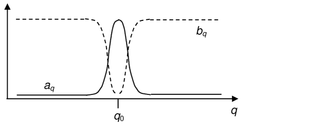
Figure 1: Typical probability distributions for long evolution times generated by selection through quantum interference.

As $t$ increases, $a_{q}(t)$ becomes more and more concentrated around $q=q_{0}$, whereas $b_{q}(t)$ will present a more and more pronounced ‘hole’ around $q=q_{0}$, as shown schematically in Fig. 1. The final state shall thus asymptotically tend to

$$a_{q_{0}}|g,q_{0}\rangle+\sum_{q\neq q_{0}}b_{q}|s,q\rangle\mathrm{.}$$ (2)

Clearly, the evolution due to the perturbation has generated an entangled state of the two degrees of freedom by selection of the $q=q_{0}$ value. Suppose one performs at large enough time $t$ a measurement of the internal state corresponding to the first degree of freedom and founds $|g\rangle$. The system is then projected onto the state $\sum_{q}a_{q}(t)|g,q\rangle$, which means that the probability of finding the system in the state $|q_{0}\rangle$ is very close to one (cf. Fig. 1). However, the probability of getting the state $|g\rangle$ as the result of the measurement is $\sum_{q}|a_{q}(t)|^{2}$ which tends to zero as $t$ increases. This ‘depopulation’ effect is the main limitation of the present method: the sharper the selection, the smaller the probability of getting the ‘good’ state selection. We shall consider in section 4 methods for controlling the depopulation of the selected states.

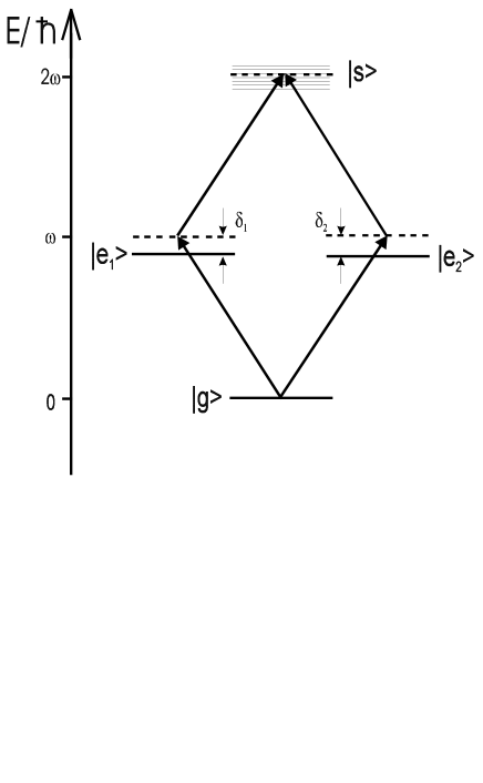
Figure 2: ‘Diamond’ level scheme for generation of quantum coherence by quantum interference. Two modes of the electromagnetic field couple the ground state $|g\rangle$ to the excited states $|s\rangle$ (that can form continuum) via two intermediate states. The two paths leading to the excited level produce quantum interference depending on the parameters of the ground state (e. g. center of mass velocity) and of the field modes (e.g. photon number).

In discussing specific examples in the following sections, we shall work essentially with the ‘diamond’ level scheme shown in Fig. 2. A quantum object called ‘the atom’ has four ‘internal’ states. States $|g\rangle$ and $|s\rangle$ are coupled by a two-photon transition via two different intermediate states $|e_{1,2}\rangle$. A mode of the electromagnetic field labeled 1 (resp. 2) couples the ground state to the intermediate state $|e_{1}\rangle$ (resp. $|e_{2}\rangle$), and the intermediate state $|e_{2}\rangle$ (resp. $|e_{1}\rangle$) to the excited state $|s\rangle$. Whether the excited state is a discrete state, a band, a continuum, or even a discrete state coupled itself to a continuum is not important here.

The excited state is connected to the ground state by two indistinguishable paths, which leads to quantum interference. Using second order perturbation, the transition rate can be written as:

$$W={n_{1}n_{2}\over\hbar^{2}}\left|{A_{1}\over\delta_{1}^{\prime}}+{A_{2}\over\delta_{2}^{\prime}}\right|^{2}$$ (3)

where $\delta_{i}^{\prime}$ is the effective detuning of the intermediate levels, which might take into account Doppler effect and/or light-shift effects, and $n_{1,2}$ are the photon number in each mode. The most general expression for the detuning we shall consider in the following is

$$\delta_{i}^{\prime}=\delta_{i}+\beta_{ii}n_{i}+\beta_{ij}n_{j}+k_{i}v$$ (4)

where $\beta_{ij}$ are light-shift coefficients (that can be easily calculated from perturbation theory), $k_{i}$ is the wavenumber of mode $i$, and $v$ the center of mass velocity. The light-shift and the Doppler effect play here the role of a ‘coupling’ between degrees of freedom linking the internal atomic state respectively to the electromagnetic field and to the center of mass motion.

Eq. (3) vanishes if

$$A_{1}\delta_{2}^{\prime}=-A_{2}\delta_{1}^{\prime}\mathrm{.}$$ (5)

The system parameters ($n_{1},n_{2}$ or $v$) appear in the expression of the detunings $\delta_{i}^{\prime}$. The above interference condition can thus be satisfied only for particular values of such parameters, and the corresponding state will be selected, as discussed above. Note however that it is not always possible to satisfy the interference condition, for example if the amplitudes $A_{1,2}$ have different complex phases. This is the principle of the method of quantum coherence generation we shall apply to specific examples in the following of the paper.

3 Generation of two-mode coherence

Let us now consider the case in which the light-shift coupling between the internal state and the field modes creates quantum coherence between the latter. We neglect the Doppler effect compared to the light-shifts in Eq. (4). The destructive interference condition deduced from Eqs. (4) and (5) is:

$$n_{2}=\alpha n_{1}+\mu$$ (6)

where

$$\alpha=-{A_{1}\beta_{22}+A_{2}\beta_{12}\over A_{1}\beta_{21}+A_{2}\beta_{22}}$$ (7)

$$\mu=-{A_{1}\delta_{2}+A_{2}\delta_{1}\over A_{1}\beta_{21}+A_{2}\beta_{22}}\mathrm{.}$$ (8)

The condition for applying the above equations is that $n_{2}\geq 0$, which means that the detunings must be chosen in the appropriate way (as the amplitudes $A_{i}$, the detunings $\delta_{i}$ and the light-shift coefficients $\beta_{ij}$ can be negative, this condition is, in general, not too hard to satisfy).

In order to simplify the notation, we take $A_{1}=-A_{2}\equiv A$. We suppose that the modes are initially ($t=t_{0}$) in uncorrelated states. The initial state of the system can thus be written in the quite general form:

$$|\psi_{0}\rangle=\sum_{n_{1},n_{2}}a(n_{1},n_{2})|g;n_{1},n_{2}\rangle$$ (9)

Because of the coupling with the level $|s\rangle$, the population of each term in the above initial state decays with a ratio given by Eq. (3). If we consider the system’s wave function $|\psi(t)\rangle$ at a latter time $t_{f}$, and project it onto the internal state $|g\rangle$ we obtain:

$$\langle g|\psi(t_{f})\rangle=\sum_{n_{1},n_{2}}\exp[-W(n_{1},n_{2})t]a(n_{1},n_{2})|g;n_{1},n_{2}\rangle$$ (10)

Clearly, for sufficiently large values of $t_{f}$, only the terms for which the interference condition Eq. (6) is satisfied, such that $W(n_{1},n_{2})t\ll 1$ will survive. Quantum interference has performed state selectiveness, and the internal ground state $|g\rangle$ has become entangled with a particular combination of photon numbers in modes 1 and 2.

In order to quantify this entanglement, consider the quantity $\delta n\equiv n_{2}-(\alpha n_{1}+\mu)$. The fluctuations of $\delta n$, $\langle\delta n^{2}\rangle-\langle\delta n\rangle^{2}$, constitute a measurement of the degree of correlation between the two modes. If the two mode are independent, the fluctuation of $\delta n$ is the sum of the fluctuations of each mode. As the modes become correlated, this quantity should go to zero. Let us thus suppose that at time $t_{f}$ one performs a measurement of the atomic state; if the result is $|g\rangle$ we measure the degree of coherence defined by the quantity:

$$R=10\log_{10}\left({\langle\delta n^{2}(t_{f})\rangle-\langle\delta n(t_{f})\rangle^{2}\over\langle\delta n^{2}(t_{0})\rangle-\langle\delta n(t_{0})\rangle^{2}}\right)\mathrm{.}$$ (11)

The smaller $R$, the greater the degree of correlation. Physically, one can interpret $R$ as the quantum noise reduction in the measurement of the quantity $\delta n$ with respect to the ‘standard limit’ corresponding to uncorrelated modes. Fig. 3 shows the time evolution of the quantity $R$ for three combinations of $(\alpha,r)$ where $r\equiv\langle n_{2}\rangle/\langle n_{1}\rangle$ is the ratio of the mean photon numbers in modes 2 and 1. We took $\mu=0$. The two modes are initially in coherent states. Some interesting features of this result can be understood in terms of rather simple arguments.

The first observation is that the degree of coherence increases when $\alpha$ increases. As the initial coherent state contains the vacuum state, there is a finite probability of finding zero photons in one of the field modes. Zero photons obviously means no transition and consequently no generation of coherence: The coherence is so to say ‘contaminated’ by the vacuum state. The probability of this ‘vacuum tail’ for coherent states decreases exponentially with the mean photon number, so that higher values of $\alpha$ correspond to higher degrees of coherence.

A second interesting feature of the result is that the degree of coherence is maximum for $r=\alpha$. This is a consequence of the ${\em filtering}$ character of the process: The weight of the filtered state in the final overall state is proportional to the weight of the filtered state in the initial overall state. This means that the final population of the state $|n_{1},\alpha n_{1}\rangle$ in the final state is proportional to the weights of the states $|n_{1}\rangle$ and $|n_{2}=\alpha n_{1}\rangle$ in the initial state, that are maxima if $\langle n_{2}\rangle\approx\alpha\langle n_{1}\rangle$ [1].

Let us finally mention that the present method can generate ‘unusual’ types of correlations between the field modes, as the following examples show. For $\alpha=1$ and $\mu=0$ one generates the usual kind of correlation obtained in parametric down conversion (that is, $n_{1}=n_{2}$). If $\alpha<0$ and $\mu\geq|\alpha|$ one should have $n_{1}\leq\mu/|\alpha|$ and $n_{2}\leq\mu$, and the resulting state is a finite superposition of number states in each mode. In particular, for $\mu=|\alpha|=1$ one should generate a one-photon number state in each mode. If $\alpha n_{1}\ll\mu$ the final state tends to the number state $n_{2}=\mu$.

If $\alpha\gg\mu$, mode 2 becomes an ‘amplified replica’ of mode 1: the quantum properties of mode 1 have been ‘cloned’ to mode 2, including quantum noise properties [2].

Closing this section, let us mention that experimental evidence of coherence generation in systems very similar to the present one has been presented by Wang, Chen and Elliot [3].

4 Atomic velocity selection

Laser cooling of neutral atoms has been a main issue of atomic physics for more then a decade now. Well understood mechanisms like Sisyphus cooling currently allows to achieve temperatures close to the so-called ‘recoil limit’. This limit corresponds to the fact that, if the average momentum transmitted to the atom by spontaneously emitted photons is zero, the root mean square value of this momentum shift is equal to the momentum $\hbar k$ of the photon. This sets a minimum energy achievable by any cooling method involving spontaneous emission to $E_{r}=\hbar^{2}k^{2}/2M$ (M is the mass of the atom), called ‘recoil energy’, to which one associates the ‘recoil temperature’ $T_{r}=\hbar^{2}k^{2}/Mk_{B}$ ($k_{B}$ is the Boltzmann’s constant). Nevertheless, it has been demonstrated that by preventing low-velocity atoms from absorbing photons it is possible achieve ‘subrecoil’ temperatures. Two such methods have been experimentally demonstrated: VSCPT (Velocity Selection by Coherent Population Trapping) [4] and Raman cooling [5]. VSCPT relies on the possibility of generating ground-state coherences which, for particular values of the atomic momentum, are uncoupled to the electromagnetic radiation due to a quantum interference effect [6]. Once the atom attains a low enough momentum, it is trapped in this momentum-defined coherent superposition and do not undergo further fluorescence cycles. We shall discuss Raman cooling in more detail in the next section.

The general method described in Sec. 2 can be applied to the generation of coherence between the internal and external (center of mass motion) degrees of freedom of an atom. By performing a measurement of the internal state, very sharp atomic velocity selection is possible. The coupling between the degree of freedom is provided by the Doppler effect. The process does not involve spontaneous emission and in principle is not limited by the recoil energy.

With counterpropagating laser beams of the same frequency, the destructive interference condition can be tuned to the velocity class $v$ by choosing (we neglect light-shift terms)

$$v={A_{1}\delta_{2}+A_{2}\delta_{1}\over(A_{2}-A_{1})k}$$ (12)

where we supposed that $A_{1}\neq A_{2}$ (otherwise destructive interference can not be achieved).

Paralleling the reasoning of the preceding section, we can write the initial wave function of the system as

$$|\psi_{0}\rangle=\int dv\,f(v)\,|g;v>\mathrm{.}$$ (13)

The transition rate $W(v)$ now depends on the velocity $v$ via the detunings $\delta_{1,2}^{\prime}=\delta_{1,2}\pm kv$, so that the projection of the asymptotic wave function over the internal state $|g\rangle$ can be written:

$$|\psi(t)\rangle=\int dv\,f(v)\,\exp[-W(v)t_{f}]\,|g;v>\mathrm{,}$$ (14)

and, again, only velocity states such that $W(v)t_{f}\ll 1$ survive.

The present case presents however a complication. Referring to Fig. 2, one sees that one must also take into account the ‘stray’ transition in which the atom absorbs one photon, goes to one of the intermediate levels and then decays back to the ground state by spontaneous emission. With a negative detuning, this process is the usual Doppler cooling whose equilibrium temperature is generally much larger then the recoil temperature. Thus, for the temperatures below the Doppler temperature which we are aiming to achieve, the ‘stray’ process heats the atoms, and competes with the velocity selection induced by the two-photon transitions. Let us just say here that it is possible, within some reasonable assumptions, to write a Fokker-Planck equation describing both one- and two-photon process (for details, see ref. [7]), from which the following conclusions can be drawn.

Fig. 4 shows the equilibrium temperature as a function of the two-photon transition rate. The excited level is supposed to be a continuum so that the two-photon transitions correspond to an irreversible ionization process. The irreversibility implies that atoms are lost as they are ionized and that the number of cooled atoms decreases along the selection process. It is shown in ref. [7] that the remaining ground-state population is proportional to $(T/T_{D})^{1/2}$. This brings about the discussion of the main limitation of the present method, namely the fact that any generation of coherence by state selection ‘looses’ a fraction of atoms that becomes larger as the selection becomes sharper. There are (at least) two ways to prevent or limit this undesirable effect, that we discuss now.

The first way of preventing depopulation is to inject into the system ‘new’ atoms in the ground state. One can then achieve an equilibrium regime in which the final selected state population is constant. It is shown in ref. [7] this scheme can produce, within experimentally realistic conditions, a significant increasing of the phase space density.

The second way to prevent depopulation is to ‘recycle’ the atoms lost in the selection process. For example, one can take a discrete excited level in Fig. 2 and let the atoms spontaneously decay back to the ground state. However, in atomic systems selection rules forbid the one-photon decay between states coupled by two-photon transitions. The allowed two-photon decay is considerably slower, thus reducing the efficiency of the selection process. A more convenient solution is to ‘fold’ the level scheme presented in Fig. 2 in such a way that the excited level becomes in fact a ground state hyperfine sublevel (see Fig. 5). We shall discuss such a system in the next section.

5 Raman cooling using quantum interference

Except in the subrecoil regime, the principle of Raman cooling is quite similar to Doppler cooling. A two-photon, Raman stimulated transition connects one ground-state sublevel to another (Fig. 5). A laser beam is used to excite a virtual intermediate level, and another beam, whose frequency differs from the first one by a value very close to the frequency interval between the two ground-state sublevel, brings the atoms to other substate by stimulated emission. As spontaneous emission is not involved in the process, the momentum transfer to the atoms is perfectly controlled: if the two beams are counterpropagating, the atomic momentum changes by $2\hbar k$ in the process. Cooling is performed by periodically exchanging the direction of the beams (or by adding two extra Raman beams [8]). Choosing a negative value for the Raman detuning $\delta_{0}$ favors the transition that cool the atoms [5] (exactly as in Doppler cooling). However, once the atom arrives in the second ground-state sublevel, it must be bought back to first one in order to allow the cooling process to proceed. This is done by ‘repumping’ the atoms with a beam resonant with the transition between the second ground-state sublevel $|f\rangle$ and the excited state. Once in the excited state, the atom has a chance of decaying to the initial ground-state sublevel $|g\rangle$ (if the atom decays to the sublevel $|f\rangle$, it will eventually be excited again, so all atoms are finally ‘repumped’ to the sublevel $|g\rangle$). As the repumping process randomizes the atomic velocity around the recoil velocity, as described above, Raman cooling cannot attain subrecoil temperatures.

To achieve the subrecoil regime, one should prevent cold enough atoms from performing Raman transitions. An atom of velocity $v$ sees an effective Raman detuning shifted by $2kv$. Using pulsed Raman excitation whose spectrum is builded such that it presents a zero for $v=0$, it is possible to decouple atoms of low enough velocity from the Raman process: Atoms within a certain range $\Delta v$ around $v=0$ are not excited. As Raman transitions are very sharp, one can have $\Delta v\ll v_{r}$. Once cooled to around the recoil velocity by the Doppler-like process, the atoms perform random walks in the velocity space until they fall into this range, where they remain trapped, and the number of trapped atoms increases as the cooling process goes on [5].

We propose an alternative method that uses quantum interference instead of spectrally shaped pulses to prevent subrecoil atoms from being excited, thus allowing continuous-wave excitation. Although hydrogen is not the most interesting atomic species in the present context, we shall consider here Raman transitions among the hyperfine sublevels of the ground state of this atom, because exact expressions for its dipole matrix elements are known, allowing the calculation of the transition rate to be easily performed [8]. Referring to Fig. 5, we can generalize Eq. (3) for hydrogen

$$Q=Q_{0}\sum_{n}{A_{n}\over{1\over q^{2}}-{1\over n^{2}}}$$ (15)

where we have used the fact that the hydrogen energy levels scales as $1/n^{2}$ ($n$ integer) and have defined $q\equiv[Ry/(\hbar\omega_{1})]^{1/2}$ ($Ry=2.2\times 10^{-18}$ J is the Rydberg). The Raman transitions amplitude is obtained by summing over all possible intermediate levels $|e_{i}\rangle$. This means that it can be possible, at least in particular cases, to choose the frequency of the Raman beams in order to produce destructive quantum interference among the contributions of the intermediate levels. The result of the calculation outlined above is presented in Fig. 6 and shows a clear pattern of resonances (corresponding to the usual resonances of the hydrogen atom) and of ‘antiresonances’ or ‘dark’ resonances, the latter corresponding to complete destructive interference. As Doppler effect displaces the position of the antiresonances, an adequate tuning the Raman beams can prevent subrecoil atoms from performing Raman transitions, thus decoupling zero-velocity atoms from the Raman process, which allows subrecoil cooling.

An interesting example of the particular dynamics of an atom under subrecoil cooling with quantum interference is presented in Fig. 7, showing the typical time evolution of the atomic velocity. It can be seen that once trapped in a low-velocity state, the atom stays there for almost the entire duration of the evolution. The statistics of the velocity states is dominated by a single state: This is the signature of a very special and interesting behavior known as ‘Levy flights’, which always manifests itself in subrecoil cooling [9].

The present method allows continuous-wave Raman subrecoil cooling, and, as the atoms can be recycled in the same way as in the usual pulsed Raman cooling, it performs subrecoil cooling without populations losses. In other words, it performs cooling instead of simply velocity selection, the repumping process insuring the dissipation necessary to the cooling process.

6 Conclusion

We have presented in a unified way a method for generation of quantum coherence though controlled state selection based on quantum interference. The application of the method to concrete examples has been discussed, concerning the generation of coherence among modes of the electromagnetic field and atomic velocity selection, in a variety of situations. Together with many other applications of quantum interference such as Velocity Selection by Coherent Population Trapping and Electromagnetically Induced Transparency, the present method illustrates the power of quantum interference as a tool for the manipulation of quantum entities.

7 Acknowledgments

The author thanks D. Hennequin, D. Wilkowski and V. Zehnlé for fruitful discussions. Laboratoire de Physique des Lasers, Atomes et Molécules (PhLAM) is Unité Mixte de Recherche 8523 du Centre National de la Recherche Scientifique (CNRS) et de l’Université des Sciences et Technologies de Lille. Centre d’Etudes et Recherches Lasers et Applications (CERLA) is supported by Ministère de la Recherche, Région Nord-Pas de Calais and Fonds Européen de Développement Economique des Régions (FEDER).

Figure 3: Time evolution of the correlation between the two modes of the electromagnetic field. The quantity $\Gamma_{0}$ is the normalized ionization rate $|A|^{2}/\hbar\omega_{0}$. Other parameters are $\langle n_{1}\rangle=100$, $\beta_{11}=\beta_{22}=10^{-4}|\delta|$, $\beta_{12}=\beta_{21}=2\times 10^{-5}|\delta|$ ($\delta$ is the detuning of the one-photon transition).

Figure 4: Dependence of the temperature (normalized to the Doppler temperature) as a function of the normalized two-photon transition rate $g=W/(v/v_{D})^{2}$, where the Doppler velocity is $v_{D}=(k_{B}T_{D}/M)^{1/2}=(\hbar\Gamma/2M)^{1/2}$. In such units, typical values of the recoil temperature range from 0.1 to 0.01 for usual atomic species. The crosses correspond to a Monte-Carlo simulation.

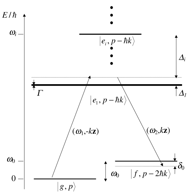
Figure 5: Levels involved in sub-recoil cooling by Raman transitions. The total Raman transition rate is proportional to the square of the sum of the contributions from each intermediate level $|e_{i}\rangle$, leading to the quantum interference effect.

Figure 6: Transition rate $Q$ for the stimulated Raman transitions between the two ground-state sublevels of the hydrogen atom. The parameter $q=\sqrt{\hbar\omega_{1}/Ry}$ coincides with an integer $n$ if the Raman excitation is resonant with the $1\rightarrow n$ transition.

Figure 7: Time evolution of the atom velocity under Raman cooling with quantum interference. The very long time the atom spends in a unique velocity state corresponds to a ‘Levy Flight’ (for $5000<\Omega_{0}t<22000$).

References

- [1] J. C. Garreau, 1996, Phys. Rev. A 53, 486.
- [2] J. A. Levenson, I. Abram, T. Rivera, P. Fayolle, J. C. Garreau and P. Grangier, 1993, Phys. Rev. Lett. 70, 267.
- [3] F. Wang, C. Chen, and D. S. Elliot, 1996, Phys. Rev. Lett. 77, 2416; C. Chen and D. S. Elliot, 1996, Phys. Rev. A 53, 272.
- [4] A. Aspect, E. Arimondo, R. Kaiser, N. Vansteenskiste, and C. Cohen-Tannoudji, 1988, Phys. Rev. Lett. 61, 826.
- [5] M. Kasevich, D. S. Weiss, E. Riis, K. Moler, S. Kasapi, and S. Chu, 1991, Phys. Rev. Lett. 66, 2297.
- [6] VSCPT is in fact a manifestation of the ‘coherence population trapping’ effect, discovered in Pisa, Italy in 1976 [G. Alzetta, A. Gozzini, L. Moi, G. Orriols, 1976, Nuovo Cimento B 36, 5]. This effect has found other interesting applications in the domain of Electromagnetically Induced Transparency (EIT) that has driven novel phenomena like lasing without inversion or the realization of ultra-hight refractive index atomic media (see, e.g., S. E. Harris, Phys. Today, July 1997, p. 36).
- [7] D. Wilkowski, J. C. Garreau, D. Hennequin, and V. Zehnlé, 1996, Phys. Rev. A 54, 4249.
- [8] J. C. Garreau, 2000, Phys. Rev. A 61, 141401(R).
- [9] F. Bardou, J. P. Bouchaud, O. Emile, A. Aspect, and C. Cohen-Tannoudji, 1994, Phys. Rev. Lett. 72, 203.