Quantum interference in optical fields and atomic radiation

Abstract

We discuss the connection between quantum interference effects in optical beams and radiation fields emitted from atomic systems. We illustrate this connection by a study of the first- and second-order correlation functions of optical fields and atomic dipole moments. We explore the role of correlations between the emitting systems and present examples of practical methods to implement two systems with non-orthogonal dipole moments. We also derive general conditions for quantum interference in a two-atom system and for a control of spontaneous emission. The relation between population trapping and dark states is also discussed. Moreover, we present quantum dressed-atom models of cancellation of spontaneous emission, amplification on dark transitions, fluorescence quenching and coherent population trapping.

1 Introduction

Optical interference is a very old technique which began with Michelson’s and Young’s experiments [1]. In these experiments, a beam of light is divided into two beams and, after traveling a distance long compared to the optical wavelength, these two beams are recombined at an observation point. If there is a small path difference between the beams, interference fringes are found at the observation point. The interference fringes are a manifestation of temporal coherence (Michelson interferometer) or spatial coherence (Young interferometer) between the two light beams. The interference experiments played a central role in early discussions of the dual nature of light, and the appearance of an interference pattern was recognized as a demonstration that light is a wave. The interpretation of the interference experiments changed with the birth of quantum mechanics, when corpuscular properties of light showed up in many experiments. According to the quantum mechanical interpretation, given by Dirac [2], the interference pattern observed in the Young’s experiment results from a superposition of the probability amplitudes of a single photon to take either of two possible pathways.

Interference effects can be observed not only between two light beams but also between radiation fields emitted from a small number of atoms or even from a single multilevel atom [3]. The interest in quantum interference in atomic system stems from the early 1970s when Agarwal [4] showed that the ordinary spontaneous decay of an excited degenerate $V$-type three-level atom can be modified due to interference between the two atomic transitions. The analysis of quantum interference has since been extended to multiatom systems and multi-level atoms. Many interesting effects have been predicted and a very wide range of practical applications have been proposed. These are too numerous to detail here, but we may mention some of the ‘traditional’ applications, such as control of optical properties of quantum systems, including high-contrast resonances [5, 6], electromagnetically induced transparency [7], lasing without inversion [8], amplification without population inversion  [9], enhancement of the index of refraction without absorption [10], and ultra-slow velocities of light [11].

In addition, quantum interference has been recognized as the most significant mechanism for the modification and suppression of spontaneous emission. The control and suppression of spontaneous emission, which is a source of undesirable noise (decoherence), is very significant in the context of quantum computation, teleportation, and quantum information processing.

The effect of quantum interference on spontaneous emission in atomic and molecular systems is the generation of superposition states which can be manipulated by adjusting the polarizations of the transition dipole moments, or the amplitudes of the external driving fields. The spontaneous emission can also be controlled by manipulating the lasers’ phases [12]. With a suitable choice of parameters, the superposition states can decay with controlled and significantly reduced rates. This modification can lead to subnatural linewidths in the fluorescence and absorption spectra [5, 13] and population trapping [14, 15]. Although the trapping states have the common property that the population will stay in such a state for an extremely long time, they can however be implemented in different ways. In a multi-level system the population can be trapped in a linear superposition of the bare atomic states, or in a dressed state corresponding to an eigenstate of the atoms plus external fields, or in some cases, in one of the excited states of the system.

In contrast to a simple theoretical picture of the effect of quantum interference on spontaneous emission in atomic systems, experimental work has proved to be extremely difficult, with only one experiment so far demonstrating the constructive and destructive interference effects in spontaneous emission [16, 18]. In the experiment they used sodium dimers, which can be modeled as five-level molecular systems with a single ground level, two intermediate and two upper levels, driven by a two-photon process from the ground level to the upper doublet. By monitoring the fluorescence from the upper levels they observed that the total fluorescent intensity, as a function of two-photon detuning, is composed of two peaks on transitions with parallel and three peaks on transitions with antiparallel dipole moments. The observed variation of the number of peaks with the mutual polarization of the dipole moments gives compelling evidence for quantum interference in spontaneous emission. Agarwal [19] has provided an intuitive picture for the observed spontaneous emission cancellation in terms of interference pathways involving a two-photon absorption process. Berman [20] has shown that the experimentally observed cancellation of spontaneous emission involving a two-photon absorption process can be interpreted in terms of population trapping. Although a cancellation of spontaneous emission is present with a two-photon excitation process, no variation of the number of peaks with the polarization of the dipole moments exist in the fluorescent intensity. Recently, Wang et al. [21] have presented a theoretical model of the observed fluorescence intensity which explains the variation of the number of the observed peaks with the mutual polarization of the molecular dipole moments.

In this paper we discuss the connection between quantum interference with optical beams and radiation fields emitted from atomic systems. We begin in Section 2 by presenting basic concepts and definitions of the first- and second-order correlation functions, which are frequently used in the analysis of the interference phenomena. Section 3 describes the master equation approach to quantum interference effects in atomic and molecular systems. In Sections 4 we discuss different methods to implement two transitions with non-orthogonal dipole moments. In Section 5, we derive general conditions for quantum interference in a two-atom system and discuss the role of the interatomic interactions. Next, in Section 6, we discuss general conditions for a control of spontaneous emission from two coupled systems and explain the relation between population trapping and dark states. In Section 7, we present quantum dressed-atom models of cancellation of spontaneous emission, amplification on dark transitions, fluorescence quenching, and coherent population trapping.

2 Optical interference and coherence

The phenomenon of optical interference is usually described in completely classical terms, in which optical fields are represented by classical plane waves. The classical theory readily explains the presence of an interference pattern in the first-order optical coherence. However, there are higher-order interference effects that distinguish the quantum nature of light from the wave nature.

2.1 First-order interference

The simplest example for a demonstration of the first-order optical interference is the Young’s double slit experiment in which two light beams of amplitudes ${\bf E}_{1}\left({\bf r}_{1},t_{1}\right)$ and ${\bf E}_{2}\left({\bf r}_{2},t_{2}\right)$, produced at two slits located at ${\bf r}_{1}$ and ${\bf r}_{2}$, respectively, incident on the screen at a point $P$, whose position vector is R. The resulting average intensity of the two fields detected at the point $P$ can be written as

$$\langle I\left({\bf R},t\right)\rangle = |u_{1}|^{2}\langle I_{1}\left({\bf R}_{1},t-t_{1}\right)\rangle+|u_{2}|^{2}\langle I_{2}\left({\bf R}_{2},t-t_{2}\right)\rangle$$ (1)

$$+2\mbox{Re}\left\{u^{\ast}_{1}u_{2}G^{(1)}\left({\bf R}_{1},t-t_{1};{\bf R}_{2},t-t_{2}\right)\right\},$$

where

$$G^{(1)}\left({\bf R}_{1},t-t_{1};{\bf R}_{2},t-t_{2}\right)=\langle{\bf E}_{1}^{\ast}\left({\bf R}_{1},t-t_{1}\right)\cdot{\bf E}_{2}\left({\bf R}_{2},t-t_{2}\right)\rangle$$ (2)

is the first order correlation function (coherence) between the field at ${\bf R}_{2}=\bf R-\bf r_{2}$ and the complex-conjugate field at ${\bf R}_{1}=\bf R-\bf r_{1}$, at times $t-t_{2}$ and $t-t_{1}$, respectively, and $u_{i}$ is a constant which depends on the geometry and the size of the $i$th slit. Here $t_{i}=R_{i}/c$.

It is convenient to introduce the normalized first-order correlation function as

$$g^{\left(1\right)}\left({\bf R}_{1},t_{1};{\bf R}_{2},t_{2}\right) = \frac{G^{\left(1\right)}\left({\bf R}_{1},t_{1};{\bf R}_{2},t_{2}\right)}{\sqrt{G^{\left(1\right)}\left({\bf R}_{1},t_{1};{\bf R}_{1},t_{1}\right)G^{\left(1\right)}\left({\bf R}_{2},t_{2};{\bf R}_{2},t_{2}\right)}}$$ (3)

$$= \frac{G^{\left(1\right)}\left({\bf R}_{1},t_{1};{\bf R}_{2},t_{2}\right)}{\sqrt{I_{1}\left({\bf R}_{1},t_{1}\right)I_{2}\left({\bf R}_{2},t_{2}\right)}},$$

satisfying the condition $0\leq|g^{\left(1\right)}|\leq 1$. The normalized correlation function (3) is often called the degree of coherence and $g^{\left(1\right)}=0$ for two independent fields, whereas $g^{\left(1\right)}=1$ for perfectly correlated fields. The intermediate values of $g^{\left(1\right)}$ $(0<|g^{\left(1\right)}|<1)$ characterize a partial coherence between the fields.

The average intensity $\langle I\left({\bf R},t\right)\rangle$ depends on $g^{\left(1\right)}$ and in the case of identical slits $(u_{1}=u_{2})$ and perfectly correlated fields $(|g^{\left(1\right)}|=1)$, the intensity can vary from $(\sqrt{I_{1}}-\sqrt{I_{2}})^{2}$ to $(\sqrt{I_{1}}+\sqrt{I_{2}})^{2}$, giving the so-called interference pattern. When $I_{1}=I_{2}=I_{0}$, the total average intensity varies from $\langle I\rangle_{min}=0$ to $\langle I\rangle_{max}=4\langle I_{0}\rangle$, giving maximal interference. For two independent fields, $g^{\left(1\right)}=0$, and then the resulting intensity is just the sum of the intensities of the two fields, that does not vary with the position of $P$.

The usual measure of the depth of modulation (sharpness) of interference fringes is the visibility in an interference pattern defined as

$${\cal{V}}\left({\bf R}\right)=\frac{\langle I\left({\bf R},t\right)\rangle_{max}-\langle I\left({\bf R},t\right)\rangle_{min}}{\langle I\left({\bf R},t\right)\rangle_{max}+\langle I\left({\bf R},t\right)\rangle_{min}},$$ (4)

where $\langle I\left({\bf R},t\right)\rangle_{max}$ and $\langle I\left({\bf R},t\right)\rangle_{min}$ represent the intensity maxima and minima at the point $P$.

Since

$$\langle I\rangle_{max}=\langle I_{1}\rangle+\langle I_{2}\rangle+2\sqrt{I_{1}I_{2}}|g^{(1)}|,$$ (5)

and

$$\langle I\rangle_{min}=\langle I_{1}\rangle+\langle I_{2}\rangle-2\sqrt{I_{1}I_{2}}|g^{(1)}|,$$ (6)

we obtain

$${\cal{V}}\left({\bf R}\right)=\frac{2\sqrt{I_{1}I_{2}}}{\left(I_{1}+I_{2}\right)}|g^{(1)}|.$$ (7)

Thus, $|g^{(1)}|$ determines the visibility of the interference fringes. In the special case of equal intensities of the two fields $(I_{1}=I_{2})$, the visibility simplifies to ${\cal{V}}\left({\bf R}\right)=|g^{(1)}|$, i.e. $|g^{(1)}|$ is then equal to the visibility. For perfectly correlated fields ${\cal{V}}\left({\bf R}\right)=1$, while ${\cal{V}}\left({\bf R}\right)=0$ for uncorrelated fields. When $I_{1}\neq I_{2}$, the visibility is always smaller than one, even for perfectly correlated fields. This fact is related to the problem of extracting which way information has been transferred through the slits into the point $P$ (welcher Weg or which-way information). The observation of an interference pattern and the acquisition of which-way information are mutually exclusive: a which-way measurement necessarily destroys the interference fringes.

We can introduce an inequality according to which the fringe visibility ${\cal{V}}$ displayed at the point $P$ and an absolute upper bound on the amount of which-way information ${\cal{D}}$ that can be detected at the point $P,$ defined as the difference in the probabilities for taking either of the two paths, are related by [22]

$${\cal{D}}^{2}+{\cal{V}}^{2}\leq 1.$$ (8)

Hence, the extreme situations characterized by perfect fringe visibility $({\cal{V}}=1)$ or full knowledge of which-way information has been transmitted $({\cal{D}}=1)$ are mutually exclusive. In order to distinguish which-way information has been transmitted, one can locate an intensity detector at the point $P$ and adjust it to measure a field of a particular intensity $I_{d}$. When the fields coming from the slits have the same intensities, the detector cannot distinguish which-way the fields came to the point $P$, so there is no which-way information available $({\cal{D}}=0)$ resulting in perfect fringe visibility $({\cal{V}}=1)$. On the other hand, when the intensities of the fields are different $(I_{1}\neq I_{2})$, the detector adjusted to measure a particular intensity can distinguish which way the field came to the point $P$ resulting in the disappearance of the interference fringes. This is clearly seen from Eq. (7): if $I_{1}\gg I_{2}$ or $I_{1}\ll I_{2}$, the visibility ${\cal{V}}\approx 0$ even for $|g^{(1)}|=1$. The same arguments apply to the frequencies and phases of the detected fields.

Information about the frequencies and phases of the detected fields is provided by the argument and phase of $g^{(1)}$. Moreover, the phase of $g^{(1)}$ determines the positions of the fringes in the interference pattern. If the observation point $P$ lies in the far field zone of the radiation emitted by the slits, the fields at the observation point can be approximated by plane waves which may be written as

$${\bf E}\left({\bf R}_{i},t-t_{i}\right)\approx{\bf E}\left({\bf R}_{i},t\right)\exp\left[-i\left(\omega_{i}t_{i}+\phi_{i}\right)\right]={\bf E}\left({\bf R}_{i},t\right)\exp\left[-i\left(\omega_{i}R_{i}/c+\phi_{i}\right)\right],\quad i=1,2,$$ (9)

where $\omega_{i}$ is the angular frequency of the $i$th field and $\phi_{i}$ is its initial phase. We can measure the frequencies from the average frequency of the two fields as

$$\omega_{1} = \omega_{0}+\frac{1}{2}\Delta,$$

$$\omega_{2} = \omega_{0}-\frac{1}{2}\Delta,$$ (10)

where $\omega_{0}=(\omega_{1}+\omega_{2})/2$ is the average frequency, and $\Delta=\omega_{1}-\omega_{2}$.

Since the observation point lies in the far field zone of the radiation emitted by the slits, i.e. the separation between the slits is very small compared to the distance to the point $P$, we can write approximately

$$R_{i}=|{\bf R}-{\bf r}_{i}|\approx R-\bar{{\bf R}}\cdot{\bf r}_{i},$$ (11)

where $\bar{{\bf R}}={\bf R}/R$ is the unit vector in the direction ${\bf R}$. Hence, substituting Eq. (9) with (10) and (11) into Eq. (3), we obtain

$$g^{\left(1\right)}\left({\bf R}_{1},t_{1};{\bf R}_{2},t_{2}\right)=|g^{\left(1\right)}\left({\bf R}_{1},t;{\bf R}_{2},t\right)|\exp\left(ik_{0}\bar{{\bf R}}\cdot{\bf r}_{21}\right)\exp\left[i\left(k_{0}\tilde{R}\frac{\Delta}{\omega_{0}}+\delta\phi\right)\right],$$ (12)

where ${\bf r}_{21}={\bf r}_{2}-{\bf r}_{1}$ is the distance between the slits, $\tilde{R}=R+\frac{1}{2}\bar{{\bf R}}\cdot\left({\bf r}_{1}+{\bf r}_{2}\right)$, $\delta\phi=\phi_{1}-\phi_{2}$, $k_{0}=\omega_{0}/c=2\pi/\lambda_{0}$, and $\lambda_{0}$ represents the mean wavelength of the fields. Let us analyze the physical meaning of the exponents appearing on the right-hand side of Eq. (12). The first exponent depends on the separation between the slits and the position ${\bf R}$ of the point $P$. For small separations the exponent changes slowly with the position ${\bf R}$ and leads to minima and maxima in the interference pattern. The minima appear whenever

$$k_{0}\bar{{\bf R}}\cdot{\bf r}_{21}=\left(2n+1\right)\pi,\quad n=0,\pm 1,\pm 2,\ldots.$$ (13)

The second exponent, appearing in Eq. (12), depends on the sum of the position of the slits, the ratio $\Delta/\omega_{0}$ and the difference $\delta\phi$ between the initial phases of the fields. This term introduces limits on the visibility of the interference pattern and can affect the pattern only if the frequencies and the initial phases of the fields are different. Even for equal and well stabilized phases, but significantly different frequencies of the fields such that $\Delta/\omega_{0}\approx 1$, the exponent oscillates rapidly with ${\bf R}$ leading to the disappearance of the interference pattern. Thus, in order to observe an interference pattern it is important to have two fields of well stabilized phases and equal or nearly equal frequencies. Otherwise, no interference pattern can be observed even if the fields are perfectly correlated.

The dependence of the interference pattern on the frequencies and phases of the fields is related to the problem of extracting which-way information. Consider the case where the two fields have mean intensities: $I_{1}=I_{2}=I_{0}.$ For perfectly correlated fields with equal frequencies $(\Delta=0)$ and equal initial phases $(\phi_{1}=\phi_{2})$, the total intensity at the point $P$ is

$$\langle I\left({\bf R}\right)\rangle=2\langle I_{0}\rangle\left(1+\cos k_{0}\bar{{\bf R}}\cdot{\bf r}_{21}\right),$$ (14)

giving an interference pattern with the maximum visibility of 100%. There are no features of the two beams which can be used to distinguish between them. For general frequencies and phases, the total intensity at the point $P$ is given by

$$\langle I\left({\bf R}\right)\rangle = 2\langle I_{0}\rangle\left[1+\left(\cos k_{0}\bar{{\bf R}}\cdot{\bf r}_{21}\right)\cos\left(k_{0}\tilde{R}\frac{\Delta}{\omega_{0}}+\delta\phi\right)\right.$$ (15)

$$-\left.\left(\sin k_{0}\bar{{\bf R}}\cdot{\bf r}_{21}\right)\sin\left(k_{0}\tilde{R}\frac{\Delta}{\omega_{0}}+\delta\phi\right)\right].$$

In this case the intensity at $P$ exhibits additional cosine and sine modulations, and at the minima the intensity is non-zero indicating that 100% modulation is not possible for two fields of different frequencies and/or initial phases. Moreover, for large frequency differences $(\Delta/\omega_{0}\gg 1)$ the cosine and sine terms oscillate rapidly with ${\bf R}$ and average to zero, washing out the interference pattern. In terms of which-way information, a detector adjusted to measure a particular frequency or phase could distinguish between the two fields. Clearly, one could tell which way the detected field came to the point $P$.

Thus, whether which-way information is available or not depends on the frequencies and phases as well as the intensities of the interfering fields. Maximum possible which-way information results in destruction of the interference pattern, and vice versa, a complete lack of which-way information results in maximum visibility of the interference pattern.

2.2 Second-order interference

The analysis of the interference phenomenon can be extended into higher-order correlation functions. The first experimental demonstration that such correlations exist in optical fields was given by Hanbury-Brown and Twiss [23], who measured the second-order correlation function of a thermal field.

The second-order (intensity) correlation function of a field of a complex amplitude ${\bf E}\left({\bf R},t\right)$ is defined as

$$G^{(2)}\left({\bf R}_{1},t_{1};{\bf R}_{2},t_{2}\right) = \langle{\bf E}^{\ast}\left({\bf R}_{1},t_{1}\right){\bf E}^{\ast}\left({\bf R}_{2},t_{2}\right){\bf E}\left({\bf R}_{2},t_{2}\right){\bf E}\left({\bf R}_{1},t_{1}\right)\rangle$$ (16)

$$= \langle I\left({\bf R}_{1},t_{1}\right)I\left({\bf R}_{2},t_{2}\right)\rangle,$$

where $I\left({\bf R}_{1},t_{1}\right)$ and $I\left({\bf R}_{2},t_{2}\right)$ are the instantaneous intensities of the field detected at a point ${\bf R}_{1}$ at time $t_{1}$ and at a point ${\bf R}_{2}$ at time $t_{2}$, respectively.

The second-order correlation function has completely different coherence properties than the first-order correlation function. An interference pattern can be observed in the second-order correlation function, but in contrast to the first-order correlation function, the interference appears between two points located at ${\bf R}_{1}$ and ${\bf R}_{2}$. Moreover, an interference pattern can be observed even if the fields are produced by two independent sources for which the phase difference $\phi_{1}-\phi_{2}$ is completely random [24]. In this case the second-order correlation function is given by

$$G^{(2)}\left({\bf R}_{1},t_{1};{\bf R}_{2},t_{2}\right)=\langle I_{1}^{2}\left(t_{1}\right)\rangle+\langle I_{2}^{2}\left(t_{2}\right)\rangle+2\langle I_{1}\left(t_{1}\right)I_{2}\left(t_{2}\right)\rangle\left[1+\cos k{\bf r}_{21}\cdot\left(\bar{{\bf R}}_{1}-\bar{{\bf R}}_{2}\right)\right].$$ (17)

Clearly, the second-order correlation function of two independent fields exhibits a cosine modulation with the separation ${\bf R}_{1}-{\bf R}_{2}$ of the two detectors. This is an interference effect although it involves a correlation function that is second order in the intensity. Similarly to the first-order correlation function, the sharpness of the fringes depends on the relative intensities of the fields. For equal intensities, $I_{1}=I_{2}=I_{0}$, the correlation function (17) reduces to

$$G^{(2)}\left({\bf R}_{1},t;{\bf R}_{2},t\right)=4\langle I_{0}^{2}\rangle\left[1+\frac{1}{2}\cos k{\bf r}_{21}\cdot\left(\bar{{\bf R}}_{1}-\bar{{\bf R}}_{2}\right)\right].$$ (18)

In analogy to the visibility in the first-order correlation function, we can define the visibility of the interference pattern of the intensity correlations as

$${\cal{V}}=\frac{G_{max}^{(2)}-G_{min}^{(2)}}{G_{max}^{(2)}+G_{min}^{(2)}},$$ (19)

and find from Eq. (18) that in the case of classical fields the maximum possible visibility of the interference pattern that can be observed is ${\cal{V}}=\frac{1}{2}$. That is, two independent fields with random and uncorrelated phases can exhibit an interference pattern in the intensity correlation with a maximum visibility of $50\%$.

2.3 Quantum interference

In the classical theory of light and coherence the field is represented by complex vectorial amplitudes ${\bf E}\left({\bf r},t\right)$ and ${\bf E}^{\ast}\left({\bf r},t\right)$, which are complex numbers (c-numbers). In the quantum theory of light the most important physical quantity is the electric field, which is represented by the field operator $\hat{{\bf E}}\left({\bf r},t\right)$. The coherence properties are discussed in terms of the negative and positive frequency parts $\hat{{\bf E}}^{(+)}$ and $\hat{{\bf E}}^{(-)}$ of the total field operator $\hat{{\bf E}}$ [25].

In the quantum description of the field, the first- and second-order correlation functions are defined in terms of the normally-ordered field operators $\hat{{\bf E}}^{(+)}$ and $\hat{{\bf E}}^{(-)}$ as

$$G^{(1)}\left({\bf R}_{1},t_{1};{\bf R}_{2},t_{2}\right) = \langle\hat{{\bf E}}^{(-)}\left({\bf R}_{1},t_{1}\right)\cdot\hat{{\bf E}}^{(+)}\left({\bf R}_{2},t_{2}\right)\rangle,$$

$$G^{(2)}\left({\bf R}_{1},t_{1};{\bf R}_{2},t_{2}\right) = \langle\hat{{\bf E}}^{(-)}\left({\bf R}_{1},t_{1}\right)\hat{{\bf E}}^{(-)}\left({\bf R}_{2},t_{2}\right)\hat{{\bf E}}^{(+)}\left({\bf R}_{2},t_{2}\right)\hat{{\bf E}}^{(+)}\left({\bf R}_{1},t_{1}\right)\rangle,$$ (20)

where the average is taken over an initial state of the field [25].

The correlation functions (20) described by the field operators are formally similar to the correlation functions (2) and (16) of the classical field. A closer examination of Eqs. (2), (16), and (20) shows that the first-order correlation functions do not distinguish between the quantum and classical theories of the electromagnetic field. However, there are significant differences between the classical and quantum descriptions of the field in the properties of the second-order correlation function [26].

As an example, consider the simple case of two single-mode fields of equal frequencies and polarizations. Assume that there are initially $n$ photons in the mode $a$ and $m$ photons in the mode $b$, and the state vectors of the fields are the Fock states $|\psi_{a}\rangle=|n\rangle$ and $|\psi_{b}\rangle=|m\rangle$. The initial state of the two fields is the direct product of the single-field states, $|\psi\rangle=|n\rangle|m\rangle$. Inserting Eq. (19) into Eq. (20) and taking the expectation value with respect to the initial state of the fields, we find

$$G^{(2)}\left({\bf R}_{1},t_{1};{\bf R}_{2},t_{2}\right)=\left(\frac{\hbar\omega}{2\epsilon_{0}V}\right)^{2}\left\{n\left(n-1\right)+m\left(m-1\right)+2nm\left[1+\cos k{\bf r}_{21}\cdot\left(\bar{{\bf R}}_{1}-\bar{{\bf R}}_{2}\right)\right]\right\}.$$ (21)

It is seen that the first two terms on the right-hand side of Eq. (21) vanish when the number of photons in each mode is smaller than 2, i.e. $n<2$ and $m<2$. In this limit the correlation function (21) reduces to

$$G^{(2)}\left({\bf R}_{1},t_{1};{\bf R}_{2},t_{2}\right)=2\left(\frac{\hbar\omega}{2\epsilon_{0}V}\right)^{2}\left[1+\cos k{\bf r}_{21}\cdot\left(\bar{{\bf R}}_{1}-\bar{{\bf R}}_{2}\right)\right].$$ (22)

Thus, perfect interference pattern with the visibility ${\cal{V}}=1$ can be observed in the second-order correlation function of two quantum fields each containing only one photon. As we have noted, the classical theory predicts a maximum visibility of ${\cal{V}}=0.5$. For $n,m\gg 1$, $m(m-1)\approx n(n-1)\approx n^{2}$, and then the quantum correlation function (21) reduces to that of the classical field.

It follows from Eq. (22) that the second-order correlation function of the quantum field vanishes when

$$k{\bf r}_{21}\cdot\left(\bar{{\bf R}}_{1}-\bar{{\bf R}}_{2}\right)=\left(2n+1\right)\pi,\quad n=0,\pm 1,\pm 2\ldots$$ (23)

In other words, two photons can never be detected at two points separated by an odd multiple of $\lambda r_{12}/2$, despite the fact that one photon can be detected anywhere. The vanishing of the second-order correlation function for two photons at widely separated points ${\bf R}_{1}$ and ${\bf R}_{2}$ is an example of quantum-mechanical nonlocality, that is the outcome of a detection measurement at ${\bf R}_{1}$ appears to be influenced by where we have chosen to locate the ${\bf R}_{2}$ detector. At certain positions ${\bf R}_{2}$ we can never detect a photon at ${\bf R}_{1}$ when there is a photon detected at ${\bf R}_{2}$, whereas at other position ${\bf R}_{2}$ it is possible. The photon correlation argument shows clearly that quantum theory does not in general describe an objective physical reality independent of observation [27].

The visibility of the fringes of the intensity correlations provides a means of testing for quantum correlations between two light fields. Mandel et al. [28] have measured the visibility in the interference of signal and idler modes simultaneously generated in the process of degenerate parametric down conversion, and observed a visibility of about $75\%$, that is a clear violation of the upper bound of $50\%$ allowed by classical correlations. Richter [29] have extended the analysis of the visibility into the third-order correlation function, and have also found significant differences in the visibility of the interference pattern of the classical and quantum fields.

3 Quantum interference in atomic systems

The phenomenon of optical interference can be observed not only between two light beams but also between radiation fields emitted from a small number of atoms or even in the radiation field emitted from a single multilevel (multi-channel) system [3, 4]. The atoms or atomic transitions can be regarded as point sources of radiation, similar to the slits in Young’s original experiment. In this case, interference results from a superposition of the transition amplitudes between quantum states of the atoms, and this phenomenon has been designated as quantum interference. The essential feature of quantum interference is the existence of linear superpositions of the atomic states which can be induced by external or internal fields, or even by the coupling of the atomic states through the environment (the vacuum field).

3.1 Correlation functions for atomic operators

Where atoms act as a source of the EM field, the correlation functions of the emitted field can be related to the correlation functions of the atomic variables, such as the atomic dipole operators.

The relation between the positive frequency part of the electric field operator at a point ${\bf R}=R\bar{{\bf R}}$, in the far-field zone, and the atomic dipole moments is given by the well-known expression [4, 30]

$$\hat{{\bf E}}^{(+)}\left({\bf R},t\right)=\hat{{\bf E}}_{0}^{(+)}\left({\bf R},t\right)-\frac{1}{c^{2}}\sum_{i=1}^{2}\frac{\bar{{\bf R}}\times\left(\bar{{\bf R}}\times\mbox{\boldmath$\mu$}_{i}\right)}{R}\omega_{i}S_{i}^{-}\left(t-\frac{R}{c}\right)\exp\left[-ik\bar{{\bf R}}\cdot{\bf r}_{i}\right],$$ (24)

where $S_{i}^{-}$ is the dipole lowering operator of the $i$th atom (dipole transition), $\mbox{\boldmath$\mu$}_{i}$ and $\omega_{i}$ are the transition dipole matrix element and the angular frequency respectively, ${\bf r}_{i}$ is the position of the $i$th atom, and $\hat{{\bf E}}_{0}^{(+)}\left({\bf R},t\right)$ denotes the positive frequency part of the field in the absence of the atoms.

If we assume that initially the field is in the vacuum state, then the free-field part $\hat{{\bf E}}_{0}^{(+)}\left({\bf R},t\right)$ does not contribute to the expectation values of the normally-ordered operators. Hence, substituting Eq.(24) into Eq.(20) and integrating over all directions ($4\pi$ solid angle) of spontaneous emission, we obtain the following expressions for the first- and second-order correlation functions

$$G^{\left(1\right)}\left({\bf R},t\right)=\sum_{i,j=1}^{2}\Gamma_{ij}\left\langle S_{i}^{+}\left(t\right)S_{j}^{-}\left(t\right)\right\rangle,$$ (25)

and

$$G^{\left(2\right)}\left({\bf R},t_{1};{\bf R},t_{2}\right)=\sum_{i,j,k,l=1}^{2}\Gamma_{il}\Gamma_{jk}\left\langle S_{i}^{+}\left(t_{1}\right)S_{j}^{+}\left(t_{2}\right)S_{k}^{-}\left(t_{2}\right)S_{l}^{-}\left(t_{1}\right)\right\rangle,$$ (26)

where $\Gamma_{ii}=\Gamma_{i}$ is the spontaneous decay rate of the $i$th transition, while $\Gamma_{ij}$ is the so-called cross-damping rate arising from the vacuum induced coupling between the two dipole moments.

For two dipole moments in a single atom, the cross-damping rate is given by

$$\Gamma_{ij}=\frac{2\sqrt{\omega_{i}^{3}\omega_{j}^{3}}}{3\hbar c^{3}}\mbox{\boldmath$\mu$}_{i}\cdot\mbox{\boldmath$\mu$}_{j}=\sqrt{\Gamma_{i}\Gamma_{j}}\cos\theta,\qquad\left(i\neq j\right),$$ (27)

where $\theta$ is the angle between the dipole moments. The cross-damping rate is sensitive to the mutual polarization of the dipole moments. If the dipole moments are parallel, $\theta=0^{o}$, and the cross-damping rate is maximal with $\Gamma_{12}=\sqrt{\Gamma_{1}\Gamma_{2}}$, whilst $\Gamma_{12}=0$ if the dipole moments are perpendicular $(\theta=90^{o})$.

In the case of two dipole transitions in two separate atoms, the cross-damping rate depends not only on the orientation of the dipole moments but also on the separation between the atoms, and is given by [4, 30]

$$\Gamma_{12} = \frac{3}{4}\sqrt{\Gamma_{1}\Gamma_{2}}\left\{\left[1-\left(\bar{\mbox{\boldmath$\mu$}}\cdot\bar{{\bf r}}_{12}\right)^{2}\right]\frac{\sin\left(k_{0}r_{12}\right)}{k_{0}r_{12}}\right.$$ (28)

$$\left.+\left[1-3\left(\bar{\mbox{\boldmath$\mu$}}\cdot\bar{{\bf r}}_{12}\right)^{2}\right]\left[\frac{\cos\left(k_{0}r_{12}\right)}{\left(k_{0}r_{12}\right)^{2}}-\frac{\sin\left(k_{0}r_{12}\right)}{\left(k_{0}r_{12}\right)^{3}}\right]\right\},$$

where $\bar{\mbox{\boldmath$\mu$}}$ is the unit vector along the dipole moments of the atoms, which we have assumed to be parallel $(\bar{\mbox{\boldmath$\mu$}}=\bar{\mbox{\boldmath$\mu$}}_{1}=\bar{\mbox{\boldmath$\mu$}}_{2})$, and $\bar{{\bf r}}_{12}$ is the unit vector along the interatomic axis. The parameter (28) is called the collective damping rate.

3.2 Master equation

There are a number of theoretical approaches that can be used to calculate quantum interference effects in atomic systems. The traditional method is the master equation approach in which the time evolution of the density operator of radiating systems is given in terms of the damping rates $\Gamma_{ij}$. For a system composed of two dipole transitions, the master equation can be written as

$$\frac{\partial}{\partial t}\rho = -\frac{i}{\hbar}\left[H_{s}+H_{sL}+H_{c},\rho\right]$$ (29)

$$-\frac{1}{2}\sum_{i,j=1}^{2}\Gamma_{ij}\left(S_{i}^{+}S_{j}^{-}\rho+\rho S_{i}^{+}S_{j}^{-}-2S_{j}^{-}\rho S_{i}^{+}\right),$$

where

$$H_{s}=\hbar\omega_{1}S_{1}^{+}S_{1}^{-}+\hbar\omega_{2}S_{2}^{+}S_{2}^{-}$$ (30)

is the Hamiltonian of the systems,

$$H_{sL}=-\frac{1}{2}\hbar\left\{\Omega_{1}S_{1}^{+}\exp\left[-i\left(\omega_{L1}t+\phi_{1}\right)\right]+\Omega_{2}S_{2}^{+}\exp\left[-i\left(\omega_{L2}t+\phi_{2}\right)\right]+{\rm H.c.}\right\}$$ (31)

is the interaction of the atomic transitions with the coherent laser fields, and

$$H_{c}=\hbar\delta_{12}^{\left(-\right)}\left(S_{1}^{+}S_{2}^{-}+S_{2}^{+}S_{1}^{-}\right)+\hbar\delta_{12}^{\left(+\right)}\left(S_{1}^{-}S_{2}^{+}+S_{2}^{-}S_{1}^{+}\right),$$ (32)

with

$$\delta_{12}^{\left(\pm\right)}=\frac{P}{\pi}\int_{-\infty}^{\infty}d\omega_{k}\frac{\Gamma_{12}}{\omega_{k}\pm\omega_{0}}$$ (33)

is the frequency shift of the atomic transitions due to their mutual interaction through the vacuum field.

In Eqs. (29)-(33), $\Omega_{1}$ and $\Omega_{2}$ are the Rabi frequencies of the laser fields of angular frequencies $\omega_{L1},\omega_{L2}$ and phases $\phi_{1},\phi_{2}$ respectively, $\omega_{0}=(\omega_{1}+\omega_{2})/2$ and $P$ stands for the principal value of the integral.

The master equation gives us an elegant description of the physics involved in the dynamics of two interacting atoms or atomic transitions. In the case of two atoms, the cross-damping rate is given in Eq. (28) and the frequency shifts $\delta_{12}^{(\pm)}$ are given by [4, 30]

$$\Omega_{12}=\delta_{12}^{(+)}+\delta_{12}^{(-)} = \frac{3}{4}\sqrt{\Gamma_{1}\Gamma_{2}}\left\{-\left[1-\left(\bar{\mbox{\boldmath$\mu$}}\cdot\bar{{\bf r}}_{21}\right)^{2}\right]\frac{\cos\left(k_{0}r_{21}\right)}{k_{0}r_{21}}\right.$$ (34)

$$\left.+\left[1-3\left(\bar{\mbox{\boldmath$\mu$}}\cdot\bar{{\bf r}}_{21}\right)^{2}\right]\left[\frac{\sin\left(k_{0}r_{21}\right)}{\left(k_{0}r_{21}\right)^{2}}+\frac{\cos\left(k_{0}r_{21}\right)}{\left(k_{0}r_{21}\right)^{3}}\right]\right\}.$$

The parameter (34) is called the retarded dipole-dipole interaction between the atoms.

In the case of two coupled transitions in a single atom, the cross-damping rate is given in Eq. (27) and $\delta_{12}^{(\pm)}$ are very small shifts of the order of the Lamb shift [31, 32]

The presence of the additional damping terms $\Gamma_{12}$ may suggest that quantum interference enhances spontaneous emission from two coupled systems. However, as we shall illustrate in the following sections, the cross-damping rate can, in fact, lead to a reduction or even suppression of spontaneous emission.

4 Implementation of two transitions with non-orthogonal dipole moments

Quantum interference between two transitions in a single atom may occur only if the dipole moments of the transitions involved are non-orthogonal, i.e.

$$\mbox{\boldmath$\mu$}_{1}\cdot\mbox{\boldmath$\mu$}_{2}\neq 0.$$

This represents a formidable practical problem, as it is very unlikely to find isolated atoms with two non-orthogonal dipole moments and quantum states close in energy. Consider, for example, a $V$-type atom with the upper states $|{1}\rangle$, $|{3}\rangle$ and the ground state $|{2}\rangle$. The evaluation of the dipole matrix elements produces the following selection rules in terms of the angular momentum quantum numbers: $J_{1}-J_{2}=\pm 1,0$, $J_{3}-J_{2}=\pm 1,0$, and $M_{1}-M_{2}=M_{3}-M_{2}=\pm 1,0$. Since in many atomic systems $M_{1}\neq M_{3}$, then $\mbox{\boldmath$\mu$}_{12}$ is perpendicular to $\mbox{\boldmath$\mu$}_{32}$ and the atomic transitions are independent. Xia et al. have found transitions with parallel and anti-parallel dipole moments in sodium molecules (dimers) and have demonstrated experimentally the effect of quantum interference on the fluorescence intensity, although their results have been criticised [16]. The transitions with parallel and anti-parallel dipole moments in the sodium dimers result from a mixing of the molecular states due to the spin-orbit coupling.

4.1 External driving field method

A mixing of atomic or molecular states can be implemented by applying external fields [17]. To illustrate this method, we consider a $V$-type atom with the upper states connected to the ground state by perpendicular dipole moments $(\mbox{\boldmath$\mu$}_{12}\perp\mbox{\boldmath$\mu$}_{32})$. When the two upper states are coupled by a resonant microwave field, the states become a linear superposition of the bare states

$$|{a}\rangle = \frac{1}{\sqrt{2}}\left(|{1}\rangle+|{3}\rangle\right),$$

$$|{b}\rangle = \frac{1}{\sqrt{2}}\left(|{1}\rangle-|{3}\rangle\right).$$ (35)

It is easy to find from Eq (35) that the dipole matrix elements between the superposition states and the ground state $|{2}\rangle$ are

$$\mbox{\boldmath$\mu$}_{a2} = \frac{1}{\sqrt{2}}\left(\mbox{\boldmath$\mu$}_{12}+\mbox{\boldmath$\mu$}_{32}\right),$$

$$\mbox{\boldmath$\mu$}_{b2} = \frac{1}{\sqrt{2}}\left(\mbox{\boldmath$\mu$}_{12}-\mbox{\boldmath$\mu$}_{32}\right).$$ (36)

When $|\mbox{\boldmath$\mu$}_{12}|\neq|\mbox{\boldmath$\mu$}_{32}|$, the dipole moments $\mbox{\boldmath$\mu$}_{a2}$ and $\mbox{\boldmath$\mu$}_{b2}$ are not perpendicular. However, the dipole moments cannot be made parallel or anti-parallel.

An alternative method in which one could create a $V$-type system with parallel or anti-parallel dipole moments is to apply a strong laser field to one of the two transitions in a $\Lambda$-type atom. The scheme is shown in Fig. 1. When the dipole moments of the $|{1}\rangle\rightarrow|{3}\rangle$ and $|{2}\rangle\rightarrow|{3}\rangle$ transitions are perpendicular, the laser exclusively couples to the $|{2}\rangle\rightarrow|{3}\rangle$ transition and produces dressed states

Figure 1: Laser induced $V$-type system with non-degenerate transitions. A laser field applied to the $|{2}\rangle-|{3}\rangle$ transition of a $\Lambda$ system creates non-degenerate dressed states separated by $\Omega=\sqrt{\Omega_{0}^{2}+\Delta^{2}_{L}}$. The sub-system with the upper dressed states $|{a}\rangle$, $|{b}\rangle$ and the ground state $|{1}\rangle$ behaves as a $V$-type system with parallel dipole moments.

$$|{a}\rangle = \sin\phi|{2}\rangle+\cos\phi|{3}\rangle,$$

$$|{b}\rangle = \cos\phi|{2}\rangle-\sin\phi|{3}\rangle,$$ (37)

where

$$\cos^{2}\phi=\frac{1}{2}+\frac{\Delta_{L}}{2\sqrt{\Omega_{0}^{2}+\Delta_{L}^{2}}},$$ (38)

$\Delta_{L}$ is the detuning of the laser frequency from the atomic transition and $\Omega_{0}$ is the on-resonance Rabi frequency of the laser field.

From Eq (37), we find that the dipole matrix elements between the dressed states and the ground state $|{1}\rangle$ are

$$\mbox{\boldmath$\mu$}_{a1} = \mbox{\boldmath$\mu$}_{13}\sin\phi,$$

$$\mbox{\boldmath$\mu$}_{b1} = \mbox{\boldmath$\mu$}_{13}\cos\phi.$$ (39)

Thus, the sub-system with the upper dressed states $|{a}\rangle,|{b}\rangle$ and the ground state $|{1}\rangle$ behaves as a $V$-type system with parallel dipole moments. This system has the advantage that the magnitudes of the transition dipole moments and the upper level splitting can be controlled by the Rabi frequency and detuning of the driving laser field.

4.2 Two-level atom in a polychromatic field

Transitions with parallel or anti-parallel dipole moments can be created not only in multi-level atoms, but also in a two-level atom driven by a polychromatic field [33]. In order to show this, we consider a two-level atom driven by a bichromatic field composed of a strong resonant laser field and a weaker laser field detuned from the atomic resonance by the Rabi frequency of the strong field. The effect of the strong field alone is to produce dressed states [34]

$$\left|1,N\right\rangle = \frac{1}{\sqrt{2}}\left(\left|g,N\right\rangle-\left|e,N-1\right\rangle\right),$$

$$\left|2,N\right\rangle = \frac{1}{\sqrt{2}}\left(\left|g,N\right\rangle+\left|e,N-1\right\rangle\right),$$ (40)

with energies $E_{1,2}=\hbar\left(N\omega_{0}\pm\frac{1}{2}\Omega\right)$, where $N$ is the number of photons in the field mode, $\Omega$ is the Rabi frequency, and $\omega_{0}$ is the atomic transition frequency.

The dressed states are shown in Fig. 2(a). We see that in the dressed atom basis the system is no longer a two-level system. It is a multi-level system with three different transition frequencies, $\omega_{0}$ and $\omega_{0}\pm\Omega$, and four nonvanishing dipole moments $\mbox{\boldmath$\mu$}_{ij,N}=\left\langle N,i\right|\mbox{\boldmath$\mu$}\left|j,N-1\right\rangle$ connecting dressed states between neighbouring manifolds

$$\mbox{\boldmath$\mu$}_{11,N}=\mbox{\boldmath$\mu$}_{12,N}=-\mbox{\boldmath$\mu$}_{21,N}=-\mbox{\boldmath$\mu$}_{22,N}=\frac{1}{2}\mbox{\boldmath$\mu$}.$$ (41)

Figure 2: (a) Dressed states of a strongly driven two-level atom. The arrows indicate the allowed spontaneous transitions with dipole moments $\pm\frac{1}{2}\mu$. (b) A second coherent field (dashed arrow) of frequency $\omega_{0}-\Omega$ couples the dipole moments of the two degenerate transitions at $\omega_{0}$.

There are two transitions with antiparallel dipole moments, $\mbox{\boldmath$\mu$}_{11,N}$ and $\mbox{\boldmath$\mu$}_{22,N}$, that oscillate with the same frequency $\omega_{0}$. This makes the system an ideal candidate for quantum interference. However, they are not coupled (correlated), preventing these dipole moments from being a source of quantum interference. This can be shown by calculating the correlation functions of the dipole moment operators of the dressed-atom transitions $\sigma_{ijN}^{+}=\left|i,N\right\rangle\left\langle N-1,j\right|,\left(i,j=1,2\right)$. The correlation functions $\left\langle\sigma_{iiN}^{+}\sigma_{jjN}^{-}\right\rangle$, $(i\neq j)$, are equal to zero, showing that the dipole moments oscillate independently.

In order to correlate them, we introduce a second (weaker) laser field of frequency $\omega_{0}-\Omega$ and Rabi frequency $\Omega_{2}<\Omega$, which couples the degenerate transitions with dipole moments $\mbox{\boldmath$\mu$}_{11,N}$ and $\mbox{\boldmath$\mu$}_{22,N-1}$, as indicated in Fig. 2(b). Treating the second field perturbatively, at zeroth order the coupling results in new “doubly-dressed” states [33]

$$\left|\bar{N},n\pm\right\rangle=\frac{1}{\sqrt{2}}\left(\left|2,N-n-1,M+n+1\right\rangle\pm\left|1,N-n,M+n\right\rangle\right),$$ (42)

where $M$ is the number of photons in the weaker field mode, and $\bar{N}=N+M$ is the total number of photons.

On calculating the transition dipole moments $\mbox{\boldmath$\mu$}_{n\pm,n\pm}$ between the doubly-dressed states, corresponding to the transitions at $\omega_{0}$, we find that the dipole moments are equal to zero. Thus, in the doubly-driven atom the effective dipole moments at $\omega_{0}$ are zero due to quantum interference between the two degenerate dipole moments of opposite phases. A consequence of this cancellation is the disappearance of the central component in the fluorescence spectrum of the doubly driven two-level atom [33].

4.3 Pre-selected polarization method

Patnaik and Agarwal [35] have proposed a method of generating a non-zero cross-damping rate in a three-level atom with perpendicular dipole moments which interacts with a single-mode cavity of a pre-selected polarization. In this system the polarization index $s$ of the cavity mode is fixed to only one of the two possible directions. This arrangement of the polarization can lead to a non-zero cross-damping term $\Gamma_{12}$ in the master equation of the system, even if the dipole moments of the atomic transitions are perpendicular. If the polarization of the cavity field is fixed, say ${\bf e}_{ks}={\bf e}_{kx}$, the polarization direction along the $x$-quantization axis, then the cross-damping rate (27) is given by

$$\Gamma_{12}=\sqrt{\Gamma_{1}\Gamma_{2}}\cos\theta_{1}\cos\theta_{2},$$ (43)

where $\theta_{j}$ is the angle between $\mbox{\boldmath$\mu$}_{j}$ and the preselected polarization vector, and usually $\theta_{1}+\theta_{2}=\pi/2$.

Zhou and Swain [36] have shown that the idea of the pre-selected polarization can be applied to engineer a system with parallel or anti-parallel dipole moments. Zhou [37] has extended the method to a cascade three-level atom coupled to a frequency-tunable cavity mode in a thermal state.

4.4 Anisotropic vacuum approach

Agarwal [38] has proposed a totally different mechanism to produce correlations between two perpendicular dipole moments. In this method the interference between perpendicular dipole moments is induced by an anisotropic vacuum field. Using second order perturbation theory, it is shown that transition probability from the ground state $|{g}\rangle$ of a four-level system to the final state $|{f}\rangle$ through two intermediate states $|{i}\rangle$ and $|{j}\rangle$ is given by

$$T_{gf}=\frac{1}{\hbar^{2}}\sum_{i,j}\Omega_{i}\Omega_{j}\frac{\mbox{\boldmath$\mu$}_{fj}^{\ast}{\bf C}\left(\omega_{L}-\omega_{fg}\right)\mbox{\boldmath$\mu$}_{fi}}{\left(\omega_{ig}-\omega_{L}\right)\left(\omega_{jg}-\omega_{L}\right)},$$ (44)

where $\Omega_{i}(\Omega_{j})$ is the Rabi frequency of the $|{g}\rangle\rightarrow|{i}\rangle(|{g}\rangle\rightarrow|{j}\rangle)$ transition, $\omega_{L}$ is the frequency of the driving laser, and ${\bf C}\left(\omega_{L}-\omega_{fg}\right)$ is the Fourier transform of the tensor, anti-normally ordered correlation function of the vacuum field operators. The anisotropy of the vacuum enters through the tensor ${\bf C}$. With perpendicular dipole moments $\mbox{\boldmath$\mu$}_{fj}$ and $\mbox{\boldmath$\mu$}_{fi}$, the transition probability responsible for the quantum interference between the $|{i}\rangle\rightarrow|{f}\rangle$ and $|{j}\rangle\rightarrow|{f}\rangle$ transitions may be non-zero only if the tensor ${\bf C}$ is anisotropic. For an isotropic vacuum the tensor ${\bf C}$ is proportional to the unit tensor and then the transition probability vanishes for $\mbox{\boldmath$\mu$}_{fi}\perp\mbox{\boldmath$\mu$}_{fj}$.

5 Quantum interference in a two-atom system

In the Young’s interference experiment the slits can be replaced by two atoms and interference effects can be observed between the coherent or incoherent fields emitted from the atoms. The advantage of using atoms instead of slits is that at a given time each atom cannot emit more than one photon. Therefore, the atoms can be regarded as sources of single photon fields.

Many interesting interference effects have been predicted in the fluorescence field emitted from two atoms, and the interference fringes have been observed experimentally in the resonance fluorescence of two trapped ions [39]. In the theoretical analysis various systems have been considered including non-identical atoms [40], the effect of interatomic interactions [41], and the dependence of the interference pattern on the direction of propagation of a driving field with respect to the interatomic axis [42].

Here, we derive general criteria for the first- and second-order interference in the fluorescence field emitted from two two-level atoms. Using these criteria, we may easily predict conditions for quantum interference in the two atom system. We consider two atoms with the upper level $|e_{i}\rangle$ and the ground level $|g_{i}\rangle$ $(i=1,2),$ located at points ${\bf r}_{1}$ and ${\bf r}_{2}$. The atoms can have identical or non-identical frequencies $\omega_{i}$ and can be coupled through the vacuum field. Moreover, the atoms may be driven by arbitrary, external fields.

Using Eq. (24), which relates the electric field operator to the atomic dipole operators, we obtain the following expressions for the time and the angular distribution of the first- and second-order correlations

$$G^{\left(1\right)}\left({\bf R},t\right) = u\left({\bf R}\right)\sum_{i,j=1}^{2}\left(\Gamma_{i}\Gamma_{j}\right)^{\frac{1}{2}}\left\langle S_{i}^{+}\left(t\right)S^{-}_{j}\left(t\right)\right\rangle\exp\left(ik\bar{{\bf R}}\cdot{\bf r}_{ij}\right),$$ (45)

$$G^{\left(2\right)}\left({\bf R},t;{\bf R},t\right) = u\left({\bf R}_{1}\right)u\left({\bf R}_{2}\right)\sum_{i,j,k,l=1}^{2}\left(\Gamma_{i}\Gamma_{j}\Gamma_{k}\Gamma_{l}\right)^{\frac{1}{2}}$$ (46)

$$\times \left\langle S^{+}_{i}\left(t\right)S^{+}_{k}\left(t\right)S^{-}_{l}\left(t\right)S^{-}_{j}\left(t\right)\right\rangle\exp\left[ik\left(\bar{{\bf R}}_{1}\cdot{\bf r}_{ij}+\bar{{\bf R}}_{2}\cdot{\bf r}_{kl}\right)\right],$$

where $u\left({\bf R}\right)$ is a constant which depends on the geometry of the system.

The traditional method to analyse coherence properties of light emitted from two atoms is to examine specific processes, such as spontaneous emission or resonance fluorescence of driven atoms. In this approach equations of motion are derived for the atomic correlation functions appearing in Eqs. (45) and (46), and solved using standard mathematical methods. Here, we present an alternative approach which allows us to identify general conditions for the observation of coherence effects without examining specific processes. In this approach, we introduce the collective states (Dicke states) of the two-atom system [15]

$$\left|g\right\rangle = \left|g_{1}\right\rangle\left|g_{2}\right\rangle,$$

$$\left|s\right\rangle = \frac{1}{\sqrt{2}}\left(\left|g_{1}\right\rangle\left|e_{2}\right\rangle+\left|e_{1}\right\rangle\left|g_{2}\right\rangle\right),$$

$$\left|a\right\rangle = \frac{1}{\sqrt{2}}\left(\left|g_{1}\right\rangle\left|e_{2}\right\rangle-\left|e_{1}\right\rangle\left|g_{2}\right\rangle\right),$$

$$\left|e\right\rangle = \left|e_{1}\right\rangle\left|e_{2}\right\rangle,$$ (47)

where $|s\rangle$ and $|a\rangle$ are the entangled symmetric and antisymmetric atomic collective states, respectively.

In the basis of the collective states (47) the atomic correlation functions, appearing in Eqs. (45) and (46), are given by

$$\left\langle S_{1}^{+}S_{1}^{-}\right\rangle+\left\langle S_{2}^{+}S_{2}^{-}\right\rangle = \rho_{ss}+\rho_{aa}+2\rho_{ee},$$

$$\left\langle S_{1}^{+}S_{2}^{-}\right\rangle = \frac{1}{2}\left(\rho_{ss}-\rho_{aa}+\rho_{as}-\rho_{sa}\right),$$

$$\left\langle S_{1}^{+}S_{2}^{+}S_{1}^{-}S_{2}^{-}\right\rangle = \rho_{ee},$$ (48)

where $\rho_{ii}(i=a,s,e)$ are the populations of the collective states and $\rho_{sa},\rho_{as}$ are coherences.

Using the relations (48), we find

$$G^{\left(1\right)}\left({\bf R},t\right) = \Gamma u\left({\bf R}\right)\left\{2\rho_{ee}\left(t\right)+\rho_{ss}\left(t\right)\left(1+\cos k\bar{{\bf R}}\cdot{\bf r}_{21}\right)\right.$$ (49)

$$+ \left.\rho_{aa}\left(t\right)\left(1-\cos k\bar{{\bf R}}\cdot{\bf r}_{21}\right)\right.$$

$$+ \left.i\left(\rho_{sa}\left(t\right)-\rho_{as}\left(t\right)\right)\sin k\bar{{\bf R}}\cdot{\bf r}_{21}\right\},$$

and

$$G^{\left(2\right)}\left({\bf R},t;{\bf R},t\right)=4\Gamma^{2}u\left({\bf R}_{1}\right)u\left({\bf R}_{2}\right)\rho_{ee}\left(t\right)\left[1+\cos k\left(\bar{{\bf R}}_{1}-\bar{{\bf R}}_{2}\right)\cdot{\bf r}_{21}\right].$$ (50)

It is evident from Eq. (49) that the first-order correlation function can exhibit an interference pattern only if $\rho_{ss}\neq\rho_{aa}$ and/or Im$(\rho_{sa})\neq 0$. This happens when $\langle e_{1}|\langle g_{2}|\rho|e_{2}\rangle|g_{1}\rangle$ and $\langle g_{1}|\langle e_{2}|\rho|g_{2}\rangle|e_{1}\rangle$ are different from zero, i.e. when there are non-zero coherences between the atoms. On the other hand, the second-order correlation function is independent of the populations $\rho_{ss},\rho_{aa}$ and the coherences, and exhibits an interference pattern when $\rho_{ee}(t)\neq 0$.

We now examine some specific processes in which one can create unequal populations of the $|s\rangle$ and $|a\rangle$ states. Dung and Ujihara  [41] have shown that spontaneous emission from two identical atoms, with initially only one atom excited, can exhibit an interference pattern. It is easy to interpret this effect in terms of the populations $\rho_{ss}(t)$ and $\rho_{aa}(t)$. If initially only one atom is excited; $\rho_{ee}(0)=\rho_{sa}(0)=\rho_{as}(0)=0$ and $\rho_{ss}(0)=\rho_{aa}(0)=\frac{1}{2}$. Using the master equation (29), we find that the time evolution of the populations $\rho_{ss}(t)$ and $\rho_{aa}(t)$ is given by

$$\rho_{ss}\left(t\right) = \rho_{ss}\left(0\right)\exp\left[-\left(\Gamma+\Gamma_{12}\right)t\right],$$

$$\rho_{aa}\left(t\right) = \rho_{aa}\left(0\right)\exp\left[-\left(\Gamma-\Gamma_{12}\right)t\right].$$ (51)

Since the populations decay with different rates, the symmetric state decays with an enhanced rate $\Gamma+\Gamma_{12}$, while the antisymmetric state decays with a reduced rate $\Gamma-\Gamma_{12}$, and the population $\rho_{aa}(t)$ is larger than $\rho_{ss}(t)$ for all $t>0$. Hence, an interference pattern can be observed for $t>0$. This effect arises from the presence of the interatomic interactions $(\Gamma_{12}\neq 0)$. Thus, for two independent atoms the populations decay with the same rate resulting in the disappearance of the interference pattern.

When the atoms are driven by a coherent laser field, an interference pattern can be observed even in the absence of the interatomic interactions. To show this, we find from the master equation (29) the steady-state solutions for the populations of the collective atomic states

$$\rho_{ee} = \frac{\Omega^{4}}{4D},$$

$$\rho_{ss} = \frac{2\Omega^{2}\left(\Gamma^{2}+\Delta_{L}^{2}\right)+\Omega^{4}}{4D},$$

$$\rho_{aa} = \frac{\Omega^{4}}{4D},$$ (52)

where $\Omega$ is the Rabi frequency of the driving field,

$$D=\Omega^{4}+\left(\Gamma^{2}+\Delta_{L}^{2}\right)\left\{\Omega^{2}+\frac{1}{4}\left[\left(\Gamma+\Gamma_{12}\right)^{2}+\left(\Delta_{L}-\Omega_{12}\right)^{2}\right]\right\},$$ (53)

and $\Delta_{L}=\omega_{0}-\omega_{L}$ is the detuning of the laser frequency from the atomic transition frequency. In the derivation of Eq. (52), we have assumed that the laser field propagates in the direction perpendicular to the interatomic axis $({\bf k}\cdot{\bf r}_{21})$ such that both atoms experience the same driving field amplitude and phase.

It is evident from Eq. (52) that $\rho_{ss}>\rho_{aa}$ even in the absence of the interatomic interactions $(\Gamma_{12}=\Omega_{12}=0)$. Hence, an interference pattern can be observed even for two independent atoms. In this case the interference pattern results from the coherent synchronization of the oscillations of the atoms by the constant coherent phase of the driving laser field.

We have shown that first-order coherence is sensitive to the interatomic interactions and the excitation field. In contrast, the second-order correlation function can exhibit an interference pattern independent of the interatomic interactions and the excitation process. According to Eq.(50), to observe an interference pattern in the second-order correlation function, it is enough to produce a non-zero population in the state $|e\rangle$. This effect results from the detection process, in that a detector does not distinguish between two simultaneously detected photons.

6 Quantum interference as a control of spontaneous emission

The master equation (29) shows that quantum interference modifies spontaneous emission rates from an atomic system. The modification and control of spontaneous emission is a topic of much current interest because of the many possible applications in quantum computation and quantum information theory. As spontaneous emission arises from the interaction of an atomic system with the vacuum field, the most obvious mechanism for modifying spontaneous emission is to place the system in a reservoir such as an electromagnetic cavity, an optical waveguide, or a photonic band-gap material. These reservoirs change the density of modes of the vacuum field into which the system can emit. For atoms in free space, quantum interference has been recognized as the basic phenomenon for controlling spontaneous emission. It was first shown by Agarwal [4] that the decay of an excited degenerate $V$-type three-level atom can be modified due to interference between the two coupled atomic transitions, and a population trapping can occur.

6.1 Vacuum-induced superposition systems

The modification of spontaneous emission from two-atom or two-channel systems results from the quantum interference induced linear superpositions of the atomic transitions. To show this, we introduce superposition operators which are linear combinations of the bare atomic dipole operators  [32]

$$S_{s}^{+} = uS_{1}^{+}+vS_{2}^{+},$$

$$S_{a}^{+} = vS_{1}^{+}-uS_{2}^{+},$$ (54)

where

$$u=\frac{\sqrt{\Gamma_{1}}}{\sqrt{\Gamma_{1}+\Gamma_{2}}},\qquad v=\frac{\sqrt{\Gamma_{2}}}{\sqrt{\Gamma_{1}+\Gamma_{2}}},$$ (55)

and $\left|u\right|^{2}+\left|v\right|^{2}=1$.

The operators $S_{s}^{+}$ and $S_{a}^{+}$ represent, respectively, symmetric and antisymmetric combinations of the dipole moments of the two systems. In terms of these new operators, the damping part of the master equation (29) may be written as

$${\cal{L}}_{d}\rho = -\Gamma_{ss}\left(S_{s}^{+}S_{s}^{-}\rho+\rho S_{s}^{+}S_{s}^{-}-2S_{s}^{-}\rho S_{s}^{+}\right)$$ (56)

$$-\Gamma_{aa}\left(S_{a}^{+}S_{a}^{-}\rho+\rho S_{a}^{+}S_{a}^{-}-2S_{a}^{-}\rho S_{a}^{+}\right)$$

$$-\Gamma_{sa}\left(S_{s}^{+}S_{a}^{-}\rho+\rho S_{s}^{+}S_{a}^{-}-2S_{a}^{-}\rho S_{s}^{+}\right)$$

$$-\Gamma_{as}\left(S_{a}^{+}S_{s}^{-}\rho+\rho S_{a}^{+}S_{s}^{-}-2S_{s}^{-}\rho S_{a}^{+}\right),$$

where

$$\Gamma_{ss} = \frac{1}{2}\frac{\left(\Gamma_{1}^{2}+\Gamma_{2}^{2}+2\Gamma_{12}\sqrt{\Gamma_{1}\Gamma_{2}}\right)}{\Gamma_{1}+\Gamma_{2}},$$

$$\Gamma_{aa} = \frac{\left(\sqrt{\Gamma_{1}\Gamma_{2}}-\Gamma_{12}\right)\sqrt{\Gamma_{1}\Gamma_{2}}}{\Gamma_{1}+\Gamma_{2}},$$

$$\Gamma_{sa} = \Gamma_{as}=\frac{1}{2}\frac{\left(\Gamma_{1}-\Gamma_{2}\right)\left(\sqrt{\Gamma_{1}\Gamma_{2}}-\Gamma_{12}\right)}{\Gamma_{1}+\Gamma_{2}}.$$ (57)

Although in general the two forms (29) and (56) look similar, the advantage of the transformed form (56) over (29) is that the damping rates of the superposition systems are significantly different even if the damping rates of the original systems are equal. When $\Gamma_{1}=\Gamma_{2}$ the damping rates satisfy $\Gamma_{sa}=\Gamma_{as}=0$, and then the symmetric and antisymmetric superpositions decay independently with rates $\frac{1}{2}\left(\Gamma+\Gamma_{12}\right)$ and $\frac{1}{2}\left(\Gamma-\Gamma_{12}\right)$ respectively. In other words, for $\Gamma_{1}=\Gamma_{2}$ the transformation (54) diagonalizes the dispersive part of the master equation. Furthermore, if $\Gamma_{12}=\sqrt{\Gamma_{1}\Gamma_{2}}$ then $\Gamma_{aa}=\Gamma_{sa}=\Gamma_{as}=0$ regardless of the ratio between $\Gamma_{1}$ and $\Gamma_{2}$. In this case the antisymmetric combination does not decay. This implies that spontaneous emission can be controlled and even suppressed by appropriately engineering the cross-damping rate $\Gamma_{12}$.

6.2 Population trapping and dark states

In the literature, population trapping is often referred to as a consequence of the cancellation of spontaneous emission. Here, we point out that the cancellation of spontaneous emission from an atomic state does not always lead to the trapping of the population in this non-decaying state. We illustrate this by considering the process of spontaneous emission from a $V$-type atom. For simplicity, we assume that spontaneous emission occurs from the excited states to the ground state with the same decay rates $\Gamma_{1}=\Gamma_{2}=\Gamma$, and the transition between the excited states is forbidden in the electric dipole approximation. The allowed transitions are represented by the dipole operators $S_{1}^{+}=\left(S_{1}^{-}\right)^{\dagger}=\left|1\right\rangle\left\langle 2\right|$ and $S_{2}^{+}=\left(S_{2}^{-}\right)^{\dagger}=\left|3\right\rangle\left\langle 2\right|$. In the absence of the driving field $(\Omega_{1}=\Omega_{2}=0)$, the master equation (29) leads to the following equations of motion for the density matrix elements

$$\dot{\rho}_{11} = -\Gamma\rho_{11}-\frac{1}{2}\Gamma_{12}\left(\rho_{13}+\rho_{31}\right),$$

$$\dot{\rho}_{33} = -\Gamma\rho_{33}-\frac{1}{2}\Gamma_{12}\left(\rho_{13}+\rho_{31}\right),$$

$$\dot{\rho}_{22} = \Gamma\left(\rho_{11}+\rho_{33}\right)+\Gamma_{12}\left(\rho_{13}+\rho_{31}\right),$$

$$\dot{\rho}_{13} = -\left(\Gamma+i\Delta\right)\rho_{13}-\frac{1}{2}\Gamma_{12}\left(\rho_{11}+\rho_{33}\right),$$

$$\dot{\rho}_{31} = -\left(\Gamma-i\Delta\right)\rho_{31}-\frac{1}{2}\Gamma_{12}\left(\rho_{11}+\rho_{33}\right),$$ (58)

where $\Delta=\omega_{1}-\omega_{2}$ is the detuning between the atomic transitions and, for simplicity, we have ignored the small frequency shifts $\delta_{12}^{(\pm)}$.

There are two different steady-state solutions of Eq. (58) depending on whether the transitions are degenerate $(\Delta=0)$ or non-degenerate $(\Delta\neq 0)$. This fact is connected with the existence of a linear combination of the density matrix elements

$$\alpha\left(t\right)=\rho_{11}\left(t\right)+\rho_{33}\left(t\right)-\rho_{13}\left(t\right)-\rho_{31}\left(t\right),$$ (59)

which, for $\Delta=0$ and $\Gamma_{12}=\Gamma$ is a constant of motion [4, 43].

In the case of $\Delta=0$ and $\Gamma_{12}=\Gamma$, the steady-state solution of Eq. (58) is

$$\rho_{11}\left(\infty\right) = \rho_{33}\left(\infty\right)=\frac{1}{4}\alpha\left(0\right),$$

$$\rho_{13}\left(\infty\right) = \rho_{31}\left(\infty\right)=-\frac{1}{4}\alpha\left(0\right),$$

$$\rho_{22}\left(\infty\right) = \frac{1}{2}\alpha\left(0\right).$$ (60)

It is seen that the steady-state population distribution depends on the initial population. When $\alpha\left(0\right)\neq 0$ a part of the population can remain in the excited states.

On the other hand, for $\Delta\neq 0$ and/or $\Gamma_{12}\neq\Gamma,$ the linear combination (59) is no longer a constant of the motion, and then the steady-state solution of Eq. (58) is

$$\rho_{11}\left(\infty\right) = \rho_{33}\left(\infty\right)=\rho_{13}\left(\infty\right)=\rho_{31}\left(\infty\right)=0,$$

$$\rho_{22}\left(\infty\right) = 1.$$ (61)

In this case the population distribution does not depend on the initial state of the atom and in the steady-state the population is in the ground state.

The properties of this system can be understood by transforming to new states which are linear superpositions of the excited atomic states

$$|{s}\rangle = \frac{1}{\sqrt{2}}\left(|{1}\rangle+|{3}\rangle\right),$$

$$|{a}\rangle = \frac{1}{\sqrt{2}}\left(|{1}\rangle-|{3}\rangle\right).$$ (62)

From Eqs. (58)and (62), we find the following equations of motion for the populations of these superposition states

$$\dot{\rho}_{ss} = -\frac{1}{2}\left(\Gamma+\Gamma_{12}\right)\rho_{ss}-\frac{1}{2}i\Delta\left(\rho_{sa}-\rho_{as}\right),$$

$$\dot{\rho}_{aa} = -\frac{1}{2}\left(\Gamma-\Gamma_{12}\right)\rho_{aa}+\frac{1}{2}i\Delta\left(\rho_{sa}-\rho_{as}\right).$$ (63)

It is seen that the antisymmetric state decays at a reduced rate $\left(\Gamma-\Gamma_{12}\right)$, and for $\Gamma_{12}=\Gamma$ the state does not decay at all. In this case the antisymmetric state can be regarded as a dark state in the sense that the state is decoupled from the environment. Secondly, we note from Eq. (63) that the population oscillates between the states with the amplitude $\Delta$, which plays here a role similar to that of the Rabi frequency of the coherent interaction between the symmetric and antisymmetric states. Consequently, an initial population in the state $|{a}\rangle$ can be coherently transferred to the state $|{s}\rangle$, which decays rapidly to the ground state. When $\Delta=0$, the coherent interaction does not take place and then any initial population in $|{a}\rangle$ will stay in this state for all times. In this case we can say that the population is trapped in the state $|{a}\rangle$.

We conclude that cancellation of spontaneous emission does not necessarily lead to population trapping. The population can be trapped in a dark state only if the state is completely decoupled from any interactions.

7 Quantum interference effects in coherently driven systems

In the preceding section, we discussed the effect of quantum interference on spontaneous emission in a two-channel system. By means of specific examples we have demonstrated that spontaneous emission can be controlled and even suppressed by quantum interference. In this section, we extend the analysis to the case of coherently driven systems. We will focus on the effect of quantum interference on transition rates between dressed states of the system. In particular, we consider coherently driven $V$ and $\Lambda$-type three-level atoms.

7.1 Excitation from an auxiliary level

Our first example for quantum interference in driven atomic systems is a three-level atom in the $V$ configuration composed of two non-degenerate excited states $\left|1\right\rangle$ and $\left|3\right\rangle$ and a single ground state $\left|2\right\rangle$. As before, we assume that the upper states $\left|1\right\rangle$ and $\left|3\right\rangle$ decay to the ground state by spontaneous emission with decay rates $\Gamma_{1}$ and $\Gamma_{2}$, respectively, whereas transitions between the excited levels are forbidden in the electric dipole approximation. The allowed transitions have dipole moments $\mbox{\boldmath$\mu$}_{12}$ and $\mbox{\boldmath$\mu$}_{32}$ sharing the same ground state $\left|2\right\rangle,$ and are represented by the operators $S_{1}^{+}=\left(S_{1}^{-}\right)^{\dagger}=\left|1\right\rangle\left\langle 2\right|$ and $S_{2}^{+}=\left(S_{2}^{-}\right)^{\dagger}=\left|3\right\rangle\left\langle 2\right|$. The transitions may be driven by a coherent laser field from an auxiliary level or the laser field may couple directly to the decaying transitions.

Zhu and Scully [44] have shown that quantum interference in a $V$-type system, driven by a laser field from an auxiliary level, can lead to the elimination of the spectral line at the driving laser frequency. The four-level system considered by Zhu and Scully is shown in Fig. 3. The laser field is coupled to non-decaying $|{1}\rangle-|{b}\rangle$ and $|{3}\rangle-|{b}\rangle$ transitions, whereas spontaneous emission occurs from the levels $|{1}\rangle$ and $|{3}\rangle$ to the ground level $|{2}\rangle$.

Figure 3: Three-level $V$-type system driven from an auxiliary level.

The most direct approach to the analysis of the dynamics of the system is the master equation (29) with the Hamiltonian $H^{\prime}$ given by

$$H^{\prime} = \hbar\omega_{1}S_{1}^{+}S_{1}^{-}+\hbar\omega_{2}S_{2}^{+}S_{2}^{-}+\hbar\omega_{b}|b\rangle\langle b|$$ (64)

$$- \frac{1}{2}\hbar\left[\left(\Omega_{1}S_{1b}^{+}+\Omega_{2}S_{3b}^{+}\right)\exp\left(-i\omega_{L}t\right)+{\rm H.c.}\right],$$

where $S_{1b}^{+}=|{1}\rangle\langle{b}|$ and $S_{3b}^{+}=|{3}\rangle\langle{b}|$ are the dipole raising operators for the transitions between the upper levels $|{1}\rangle$ and $|{3}\rangle$ and the auxiliary level $|{b}\rangle$.

The spectrum of the fluorescence field emitted on the $|{1}\rangle\rightarrow|{2}\rangle$ and $|{3}\rangle\rightarrow|{2}\rangle$ transitions is given by the Fourier transform of the two-time correlation function of the dipole moments of the transitions that, according to the quantum regression theorem [45], satisfy the same equations of motion as the density matrix elements $\rho_{12}(t)$ and $\rho_{32}(t)$. Using the master equation (28) with the Hamiltonian (64), we obtain the following set of coupled equations of motion for the density matrix elements

$$\frac{\partial}{\partial t}{\bf X}\left(t\right)=M{\bf X}\left(t\right),$$ (65)

where ${\bf X}\left(t\right)=[\rho_{12}(t),\rho_{32}(t),\rho_{b2}(t)]$ is a column vector composed of the density matrix elements, and $M$ is the $3\times 3$ matrix

$$M=\left(\begin{array}[]{ccc}-(\frac{1}{2}\Gamma_{1}+i\Delta_{1})&-\frac{1}{2}\Gamma_{12}&\frac{1}{2}i\Omega_{1}\\ -\frac{1}{2}\Gamma_{12}&-(\frac{1}{2}\Gamma_{2}+i\Delta_{2})&\frac{1}{2}i\Omega_{2}\\ \frac{1}{2}i\Omega_{1}&\frac{1}{2}i\Omega_{2}&0\end{array}\right),$$ (66)

where $\Delta_{1}=\omega_{1b}-\omega_{L}$ and $\Delta_{2}=\omega_{3b}-\omega_{L}$ are the detunings of the laser field from the $|{1}\rangle-|{b}\rangle$ and $|{3}\rangle-|{b}\rangle$ transitions, respectively. Following Zhu and Scully, we assume that $\Gamma_{1}=\Gamma_{2}=\Gamma$, $\Omega_{1}=\Omega_{2}=\Omega$ and that the laser field is tuned to the middle of the upper levels spitting, i.e. $\Delta_{2}=-\Delta_{1}=\frac{1}{2}\Delta$.

Since we are interested in the time evolution of the density matrix elements, we need explicit expressions for the components $X_{i}$ of the vector ${\bf X}\left(t\right)$ in terms of their initial values. This can be done by a direct integration of (65). Thus, if $t_{0}$ denotes an arbitrary initial time, the integration of (65) leads to the following formal solution for ${\bf X}\left(t\right)$

$${\bf X}\left(t\right)={\bf X}\left(t_{0}\right)\exp\left(Mt\right).$$ (67)

Because the determinant of the matrix $M$ is different from zero, there exists a complex invertible matrix $T$ which diagonalises $M$, and $\lambda=T^{-1}MT$ is the diagonal matrix of complex eigenvalues, which can be found from the eigenvalue equation

$$\lambda\left[\lambda^{2}+\Gamma\lambda+\frac{1}{4}\Delta^{2}+\frac{1}{4}\left(\Gamma^{2}-\Gamma_{12}^{2}\right)\right]+\frac{1}{2}\Omega^{2}\left[\lambda+\frac{1}{2}\left(\Gamma-\Gamma_{12}\right)\right]=0.$$ (68)

There are two different solutions of Eq. (68) depending on whether $\Gamma_{12}=\Gamma$ or $\Gamma_{12}\neq\Gamma$. For $\Gamma_{12}=\Gamma$, which corresponds to parallel dipole moments of the transitions, and $\Omega\gg\Gamma$ the roots of the cubic equation (68) are

$$\lambda_{1} = 0,$$

$$\lambda_{2} = -\frac{1}{2}\Gamma+i\Omega^{\prime},$$

$$\lambda_{3} = -\frac{1}{2}\Gamma-i\Omega^{\prime},$$ (69)

whilst for $\Gamma_{12}=0$, which corresponds to perpendicular dipole moments, and $\Omega\gg\Gamma$ the roots are

$$\lambda_{1} = -\frac{1}{2}\Gamma,$$

$$\lambda_{2} = -\frac{1}{4}\Gamma+i\Omega^{\prime},$$

$$\lambda_{3} = -\frac{1}{4}\Gamma-i\Omega^{\prime},$$ (70)

where $\Omega^{\prime}=\frac{1}{2}\sqrt{\Delta^{2}+2\Omega^{2}}$.

Thus, in the case of parallel dipole moments, the spectrum is composed of two lines of equal bandwidths $(\frac{1}{2}\Gamma)$ located at frequencies $\pm\Omega^{\prime}$ and there is no central component in the fluorescence spectrum at the laser frequency $\omega_{L}$. The eigenvalue $\lambda=0$ contributes to the coherent scattering of the laser field. When $\Gamma_{12}=0$, the spectrum is composed of three lines: the central line of the bandwidth $\frac{1}{2}\Gamma$ located at the laser frequency and two sidebands of bandwidths $\frac{1}{4}\Gamma$ located at $\pm\Omega^{\prime}$. The absence of the central line for $\Gamma_{12}=\Gamma$ is clear evidence of the cancellation of spontaneous emission into the vacuum modes around the laser frequency by quantum interference.

The physical origin of the cancellation of the central line in the spectrum can be explained clearly by the dressed-atom model of the system [34, 46]. In this model we use a fully quantum-mechanical description of the Hamiltonian of the system, which in a frame rotating with the laser frequency $\omega_{L}$ can be written as

$$H^{\prime}=H_{0b}+V_{b},$$ (71)

where

$$H_{0b}=\hbar\Delta_{1}S_{1}^{+}S_{1}^{-}+\hbar\Delta_{2}S_{2}^{+}S_{2}^{-}+\hbar\omega_{L}a_{L}^{\dagger}a_{L},$$ (72)

is the Hamiltonian of the uncoupled system and the laser field, and

$$V_{b}=-\frac{\hbar}{2}g\left[\left(S_{1b}^{+}+S_{2b}^{+}\right)a_{L}+a_{L}^{\dagger}\left(S_{1b}^{-}+S_{2b}^{-}\right)\right]$$ (73)

is the interaction of the laser with the atom. In Eq. (73), $g$ is the system-field coupling constant, and $a_{L}$ $(a_{L}^{\dagger})$ is the annihilation (creation) operator for the driving field mode.

For $\Delta_{2}=-\Delta_{1}=\frac{1}{2}\Delta$, the Hamiltonian $H_{0b}$ has four non-degenerate eigenstates $\left|2,N\right\rangle,$ $\left|b,N\right\rangle$, $\left|1,N-1\right\rangle$, and $\left|3,N-1\right\rangle$, where $\left|i,N\right\rangle$ is the state with the atom in state $\left|i\right\rangle$ and $N$ photons present in the driving laser mode. When we include the interaction $V_{b}$, the diagonalization of the Hamiltonian $H_{0b}+V_{b}$ leads to the following dressed states of the system

$$\left|+,N\right\rangle = \frac{1}{2}\left[\left(1-\alpha\right)\left|1,N-1\right\rangle+\left(1+\alpha\right)\left|3,N-1\right\rangle-2\beta\left|b,N\right\rangle\right],$$

$$\left|0,N\right\rangle = -\beta\left(\left|1,N-1\right\rangle-\left|3,N-1\right\rangle\right)+\alpha\left|b,N\right\rangle,$$

$$\left|-,N\right\rangle = \frac{-1}{2}\left[\left(1+\alpha\right)\left|1,N-1\right\rangle+\left(1-\alpha\right)\left|3,N-1\right\rangle+2\beta\left|b,N\right\rangle\right],$$

$$\left|2,N\right\rangle = \left|2,N\right\rangle$$ (74)

with energies

$$E_{N,+} = \hbar\left(N\omega_{L}+\Omega^{\prime}\right),$$

$$E_{N,0} = \hbar N\omega_{L},$$

$$E_{N,-} = \hbar\left(N\omega_{L}-\Omega^{\prime}\right),$$

$$E_{N,2} = \hbar N\omega_{L},$$ (75)

where $\alpha=\Delta/2\Omega^{\prime}$ and $\beta=\Omega/2\Omega^{\prime}$.

Figure 4: Dressed states of two neighboring manifolds, $N+1$ and $N$. Solid arrows indicate transitions at $\omega_{L}\pm\Omega^{\prime}$ which are only slightly affected by quantum interference, while the dashed arrow indicates the transition at the laser frequency $\omega_{L}$ which is strongly affected by quantum interference and vanishes for parallel dipole moments and $|\mbox{\boldmath$\mu$}_{12}|=|\mbox{\boldmath$\mu$}_{32}|$.

Dressed states of two neighbouring manifolds are shown in Fig. 4. The manifolds are separated by $\omega_{L}$, while the states inside each manifold are separated by $\Omega^{\prime}$. The dressed states are connected by transition dipole moments. It is easily verified that non-zero dipole moments occur only between states within neighbouring manifolds. Defining transition dipole moments $\mbox{\boldmath$\mu$}_{i,N+1;2,N}=\left\langle N+1,i\right|\mbox{\boldmath$\mu$}\left|2,N\right\rangle$ between $\left|i,N+1\right\rangle$ $(i=0,-,+)$ and $\left|2,N\right\rangle,$ and using Eq. (74), we find

$$\mbox{\boldmath$\mu$}_{+,N+1;2,N} = \left(1-\alpha\right)\mbox{\boldmath$\mu$}_{12}+\left(1+\alpha\right)\mbox{\boldmath$\mu$}_{32},$$

$$\mbox{\boldmath$\mu$}_{0,N+1;2,N} = -\beta\left(\mbox{\boldmath$\mu$}_{12}-\mbox{\boldmath$\mu$}_{32}\right),$$

$$\mbox{\boldmath$\mu$}_{-,N+1;2,N} = -\left[\left(1+\alpha\right)\mbox{\boldmath$\mu$}_{12}+\left(1-\alpha\right)\mbox{\boldmath$\mu$}_{32}\right].$$ (76)

The transition dipole moments $\mbox{\boldmath$\mu$}_{2,N;i,N-1}$ between $\left|2,N\right\rangle$ and the dressed states $\left|i,N-1\right\rangle$ of the manifold below are equal to zero, independent of the mutual orientation of the atomic dipole moments. It is evident from Eq. (76) that transitions to the state $\left|2,N\right\rangle$ depend on the mutual polarization of the dipole moments $\mbox{\boldmath$\mu$}_{12}$ and $\mbox{\boldmath$\mu$}_{32}$. For $\mbox{\boldmath$\mu$}_{12}\parallel\mbox{\boldmath$\mu$}_{32}$ and $|\mbox{\boldmath$\mu$}_{12}|=|\mbox{\boldmath$\mu$}_{32}|$ the transition dipole moment $\mbox{\boldmath$\mu$}_{0,N+1;2,N}$ vanishes, resulting in the disappearance of the central component of the fluorescence spectrum. When $\mbox{\boldmath$\mu$}_{12}$ and $\mbox{\boldmath$\mu$}_{32}$ are not parallel, all the transitions are allowed, and three lines can be seen in the spectrum.

It is interesting to note that in the case of antiparallel dipole moments and $\Delta=0$ the dipole moments $\mbox{\boldmath$\mu$}_{+,N+1;2,N}$ and $\mbox{\boldmath$\mu$}_{-,N+1;2,N}$ vanish, resulting in the disappearance of the Rabi sidebands of the spectrum. Thus, depending on the polarization of the dipole moments and the splitting $\Delta$, the spectrum can exhibit, one, two or three spectral lines. The dressed-atom model clearly explains the origin of the cancellation of the spectral lines. This effect arises from the cancellation of the transition dipole moments due to quantum interference between the two atomic transitions.

7.2 Excitation of a single transition

Here, we consider a three-level $V$-type atom driven by a strong laser field of Rabi frequency $\Omega$, coupled solely to the $\left|1\right\rangle-\left|2\right\rangle$ transition. This is a crucial assumption, which would be difficult to realize in practice since quantum interference requires almost parallel dipole moments. However, the difficulty can be overcome in atomic systems with specific selection rules for the transition dipole moments, or by applying fields with specific polarization properties [47].

In addition, we assume that the atom is probed by a weak laser field. We consider two different coupling configurations of the probe beam to the driven atom. In the first case, we assume that the probe beam is exclusively coupled to the driven $\left|1\right\rangle\rightarrow\left|2\right\rangle$ transition [48]. In the second case, we will assume that the probe beam is coupled to the undriven $\left|3\right\rangle\rightarrow\left|2\right\rangle$ transition. For the second case, Menon and Agarwal [49] have predicted that in the presence of quantum interference the absorption spectrum of the probe beam can exhibit gain features instead of the usual Autler-Townes doublet. This unexpected feature requires the condition that the driving field couples to only one of the two atomic transitions and the Rabi frequency $\Omega$ of the driving field is such that $\Omega=2\Delta$, where $\Delta$ is the splitting between the excited states.

The absorption rate of a probe beam of a tunable frequency $\omega_{p}$ monitoring the $\left|1\right\rangle-\left|2\right\rangle$ transition is defined as [49, 50]

$$W_{12}\left(\omega_{p}\right)={\rm Re}\left[\Omega_{p}\rho_{12}^{\left(+1\right)}\right],$$ (77)

where $\Omega_{p}$ is the Rabi frequency of the probe beam, and $\rho_{12}^{\left(+1\right)}$ is the stationary component (harmonic) of the coherence $\rho_{12}$ oscillating with the probe detuning $\delta=\omega_{p}-\omega_{2}$.

Figure 5: The absorption rate $W_{12}$ as a function of $\delta/\Gamma_{1}$ for $p=0.95,\Gamma_{1}=\Gamma_{2},\Omega_{p}=0.5\Gamma_{1},\Delta=15\Gamma_{1}$ and different $\Omega$: $\Omega=10\Gamma_{1}$ (solid line) and $\Omega=30\Gamma_{1}$ (dashed line).

In Fig. 5, we plot the absorption rate $W_{12}$ as a function of $\delta$ for $p=0.95$ and different $\Omega$. When $\Omega\neq 2\Delta$ the absorption rate exhibits the familiar Mollow absorption spectrum [50] with small dispersive structures at $\delta=\pm\Omega$. The absorption rate changes dramatically when $\Omega=2\Delta$. Here, the dominant features of the rate are emissive and absorptive components at $\delta=\pm\Omega$, indicating that at $\delta=-\Omega$ the weaker field is absorbed, whereas at $\delta=\Omega$ it is amplified at the expense of the strong field. The weaker field is always absorbed (amplified) at $\delta=-\Omega$ $(\delta=\Omega)$ independent of the ratio $r=\Gamma_{1}/\Gamma_{2}$ between the spontaneous emission rates $\Gamma_{1}$ and $\Gamma_{2}$. Note that the absorption rate shown in Fig. 5 is similar to the Mollow absorption spectrum for an off-resonant driving field [50]. However, there is a significant difference in that the ratio between the magnitudes of the emissive and absorptive peaks in the Mollow spectrum is always less than one and the ratio varies with the detuning and Rabi frequency of the driving field. The ratio of the absorption rates, shown in Fig. 5, is equal to one and constant independent of the values of the parameters involved.

Figure 6: The absorption rate $W_{23}$ as a function of $\delta$ for $\Omega=30\Gamma_{1}$, $\Omega_{p}=0.5\Gamma_{1}$, $\Delta=15\Gamma_{1}$, $p=0.95$ and different values of $r$: $r=1$ (solid line), $r=2$ (dashed line) and $r=5$ (dashed-dotted line).

In Fig. 6, we present the absorption rate for the case considered by Menon and Agarwal [49], in which the probe beam is coupled to the undriven $|3\rangle-|2\rangle$ transition

$$W_{23}\left(\omega_{p}\right)=2{\rm Re}\left[\Omega_{p}\rho_{23}^{\left(+1\right)}\right].$$ (78)

The absorption rate is plotted as a function of $\delta$ for $\Omega=2\Delta$. We see that the absorption rate exhibits an emissive feature at $\delta=\Omega$. Moreover, there is a central component at $\delta=0$, whose absorptive/emissive properties depend on the ratio $r$. For $r<2$ the rate is positive, indicating that the weaker field is absorbed by the system. As $r$ increases the absorptive feature decreases and vanishes for $r\approx 2$. When we further increase $r$ $(r>2)$ the absorptive features at $\delta=0$ switch into emissive features and the magnitude of the emissive peak increases with increasing $r$. The threshold value for $r$, at which absorption switches to emission, depends on $p$. For $p=1$ the threshold is exactly at $r=2$, and shifts towards larger $r$ as $p$ decreases.

The physics associated with the unusual properties of the absorption rate of the probe beam, shown in Figs. 5 and 6, can be easily explored by working in the basis of quantum dressed states of the system [51]. In the case of the driving laser coupled exclusively to the $|1\rangle-|2\rangle$ transition, the Hamiltonian of the system can be written as

$$H_{S}=H_{0}+H_{int},$$ (79)

where

$$H_{0}=\hbar\omega_{1}S_{1}^{+}S_{1}^{-}+\hbar\omega_{2}S_{2}^{+}S_{2}^{-}+\hbar\omega_{1}a_{L_{1}}^{\dagger}a_{L_{1}},$$ (80)

is the Hamiltonian of the atom plus driving field, and

$$H_{int}=-\frac{1}{2}\hbar g\left(a_{L_{1}}^{\dagger}S_{1}^{-}+a_{L_{1}}S_{1}^{+}\right)$$ (81)

is the interaction between the atom and the laser field.

The Hamiltonian $H_{0}$ has the “undressed” eigenstates $|1,N-1\rangle,|3,N-1\rangle$ and $|2,N\rangle$. The states $|1,N-1\rangle$ and $|2,N\rangle$ are degenerate with energies $E_{1,N}=E_{2,N}=\hbar\omega_{1}$, while the state $|3,N-1\rangle$ has energy $E_{3,N}=\hbar(N\omega_{1}+\Delta)$, where $N$ is the number of photons in the laser mode. When we include the interaction (81) between the atom and the laser field, the degeneracy is lifted, resulting in triplets of dressed states

$$|+,N\rangle = \frac{1}{\sqrt{2}}\left(|2,N\rangle+|1,N-1\rangle\right),$$

$$|-,N\rangle = \frac{1}{\sqrt{2}}\left(|2,N\rangle-|1,N-1\rangle\right),$$

$$|\tilde{3},N\rangle = |3,N-1\rangle,$$ (82)

with energies

$$E_{+,N} = \hbar\left(N\omega_{1}+\frac{1}{2}\Omega\right),$$

$$E_{-,N} = \hbar\left(N\omega_{1}-\frac{1}{2}\Omega\right),$$

$$E_{\tilde{3},N} = \hbar\left(N\omega_{1}+\Delta\right).$$ (83)

The dressed states (82) group into manifolds of nondegenerate triplets unless $\Delta=\frac{1}{2}\Omega$ and then the states $|+,N\rangle$, $|\tilde{3},N\rangle$ in each manifold are degenerate.

Since the driven and undriven transitions are coupled through the $\Gamma_{12}$ terms, it is convenient to introduce symmetric and anti-symmetric superposition states of the dressed states $|+,N\rangle$ and $|\tilde{3},N\rangle$. According to Eq. (83), the superposition states diagonalise the dissipative (damping) part of the master equation of the system. The superposition states can be written as [48]

$$|s,N\rangle = \alpha|+,N\rangle+\beta|\tilde{3},N\rangle,$$ (84)

$$|a,N\rangle = \beta|+,N\rangle-\alpha|\tilde{3},N\rangle,$$ (85)

where

$$\alpha=\frac{1}{\sqrt{1+2r}},\beta=\frac{\sqrt{2r}}{\sqrt{1+2r}},$$ (86)

and $r=\Gamma_{2}/\Gamma_{1}$.

With the dressed states of the driven system available, we may easily predict transition frequencies and calculate transition dipole moments and spontaneous emission rates between the dressed states of the system. It is easily verified that non-zero dipole moments occur only between dressed states within neighbouring manifolds. Using Eqs. (84) and (85), we find that the transition dipole moments between $|N,i\rangle$ and $|N-1,j\rangle$ are

$$\mbox{\boldmath$\mu$}_{s,N;s,N-1} = \frac{1}{2}\alpha\left(\alpha\mbox{\boldmath$\mu$}_{12}+\sqrt{2}\beta\mbox{\boldmath$\mu$}_{32}\right),\quad\mbox{\boldmath$\mu$}_{s,N;-,N-1}=\frac{1}{2}\left(\alpha\mbox{\boldmath$\mu$}_{12}+\sqrt{2}\beta\mbox{\boldmath$\mu$}_{32}\right),$$

$$\mbox{\boldmath$\mu$}_{-,N;s,N-1} = -\frac{1}{2}\alpha\mbox{\boldmath$\mu$}_{12},\quad\mbox{\boldmath$\mu$}_{-,N;-,N-1}=-\frac{1}{2}\mbox{\boldmath$\mu$}_{12},$$

$$\mbox{\boldmath$\mu$}_{-,N;a,N-1} = -\frac{1}{2}\beta\mbox{\boldmath$\mu$}_{12},\quad\mbox{\boldmath$\mu$}_{s,N;a,N-1}=\frac{1}{2}\beta\left(\alpha\mbox{\boldmath$\mu$}_{12}+\sqrt{2}\beta\mbox{\boldmath$\mu$}_{32}\right),$$

$$\mbox{\boldmath$\mu$}_{a,N;s,N-1} = \frac{1}{2}\alpha\left(\beta\mbox{\boldmath$\mu$}_{12}-\sqrt{2}\alpha\mbox{\boldmath$\mu$}_{32}\right),\quad\mbox{\boldmath$\mu$}_{a,N;-,N-1}=\frac{1}{2}\left(\beta\mbox{\boldmath$\mu$}_{12}-\sqrt{2}\alpha\mbox{\boldmath$\mu$}_{32}\right),$$

$$\mbox{\boldmath$\mu$}_{a,N;a,N-1} = \frac{1}{2}\beta\left(\beta\mbox{\boldmath$\mu$}_{12}-\sqrt{2}\alpha\mbox{\boldmath$\mu$}_{32}\right),$$ (87)

where $\mbox{\boldmath$\mu$}_{i,N;j,N-1}=\langle i,N|\tilde{\mbox{\boldmath$\mu$}}|j,N-1\rangle$, and $\tilde{\mbox{\boldmath$\mu$}}=\tilde{\mbox{\boldmath$\mu$}}_{1}+\tilde{\mbox{\boldmath$\mu$}}_{2}$ is the total dipole moment of the atom.

The spontaneous transitions occur with probabilities $\Gamma_{i,N;j,N-1}$ given by

$$\Gamma_{i,N;j,N-1}=\frac{\Gamma_{n}}{\left|\mbox{\boldmath$\mu$}_{2n-1,2}\right|^{2}}\left|\left\langle i,N\right|\tilde{\mbox{\boldmath$\mu$}}\left|j,N-1\right\rangle\right|^{2},\quad n=1,2,$$ (88)

Figure 7: Energy level diagram of the superposition dressed states for $\Delta=\frac{1}{2}\Omega$. The solid lines indicate spontaneous transitions which occur independent of quantum interference, whereas the dash ed lines indicate transitions which are significantly reduced by quantum interference.

In Fig. 7, we present the dressed states of two neighbouring manifolds, $N$ and $N-1$, and the possible transitions among them. Solid lines indicate transitions which are not significantly affected by quantum interference, whereas dashed lines indicate transitions which are strongly modified by quantum interference, in that their transition dipole moments decrease with increasing $p$ and vanish for $p=1$. We see from Fig. 7 that quantum interference strongly affects transition rates from the antisymmetric state to the states of the manifold below. Thus, the antisymmetric state becomes a dark state in the limit of strong interference, $p\approx 1$. Moreover, it follows from the master equation (29) and the dressed state (85) that in the steady-state the antisymmetric state is strongly populated, and the population is trapped in the antisymmetric state $(P_{a}=1)$ when $\theta=0$.

Figure 7, together with the transition dipole moments and transition rates, provides a simple interpretation of the absorption rate shown in Fig. 5. Since the antisymmetric state is strongly populated, the emissive peak in the absorption rate appears on an almost completely inverted transition $(|a,N\rangle-|-,N-1\rangle)$, whose dipole moment is significantly reduced by quantum interference. One might expect that the weaker field should not couple to an almost canceled dipole moment. However, we have assumed that the probe field couples only to the dipole moment $\mbox{\boldmath$\mu$}_{12}$. From Eq. (87), we find that the coupling strength of the probe field to the transition $|a,N\rangle-|-,N-1\rangle$ is proportional to $\frac{1}{2}\beta\mbox{\boldmath$\mu$}_{12}$ despite the fact that the total dipole moment of the transition is much smaller, $\mbox{\boldmath$\mu$}_{a,N;-,N-1}=\frac{1}{2}\beta\mbox{\boldmath$\mu$}_{12}-\frac{1}{\sqrt{2}}\alpha\mbox{\boldmath$\mu$}_{32}$. The absorptive peak, seen in Fig. 5 at the frequency $\omega_{1}-\Omega$, appears on the non-inverted transition $|-,N\rangle-|a,N-1\rangle$ with the transition dipole moment $\frac{1}{2}\beta\mbox{\boldmath$\mu$}_{12}$. Since the absolute values of the population difference on the $|a,N\rangle-|-,N-1\rangle$ and $|-,N\rangle-|a,N-1\rangle$ transitions are the same and the coupling strengths of the weaker field to the transitions are equal, $\mbox{\boldmath$\mu$}_{a,N;-,N-1}=\mbox{\boldmath$\mu$}_{-,N;a,N-1}=\frac{1}{2}\beta\mbox{\boldmath$\mu$}_{12}$, the absolute values of the absorptive and emissive peaks in the absorption rate are the same, independent of the ratio $r=\Gamma_{1}/\Gamma_{2}$. One sees from Fig. 7 that there are two transitions, one emissive $(|a,N\rangle-|s,N-1\rangle)$ and one absorptive $(|s,N\rangle-|a,N-1\rangle)$, which contribute to the central structure at $\delta=0$. Since the absolute values of the population difference on these transitions are the same and the coupling strengths of the weaker field to these transitions are equal, $\mbox{\boldmath$\mu$}_{s,N;a,N-1}=\mbox{\boldmath$\mu$}_{a,N;s,N-1}=\frac{1}{2}\alpha\beta\mbox{\boldmath$\mu$}_{12}$, these two contributions cancel each other leading to a transparency of the weaker field at $\delta=0$.

The physical origin of the gain features shown in Fig. 6 can also be explained with the help of the energy-level diagram of Fig. 7 and the transition dipole moments (87). Since the weaker field couples exclusively to $\mbox{\boldmath$\mu$}_{32}$, the transition $\left|a,N-1\right\rangle-\left|-,N\right\rangle$, whose dipole moment is proportional to $\mbox{\boldmath$\mu$}_{12}$, is transparent for the weaker field. The coupling strength of the weaker field to the $\left|a,N\right\rangle-\left|-,N-1\right\rangle$ transition is proportional to ${\displaystyle{1\over\sqrt{2}}}\alpha\mbox{\boldmath$\mu$}_{32}$ indicating that the field can be amplified on this transition and the amplification is not much affected by the the ratio $r$. It is seen from Fig. 7 that at $\delta=0$ the probe couples to three transitions. The transition $\left|a,N\right\rangle-\left|a,N-1\right\rangle$ is transparent for the probe because it occurs between two states of the same population. Therefore, the absorptive/emissive properties result from the coupling of the probe to the $\left|s,N\right\rangle-\left|a,N-1\right\rangle$ and $\left|a,N\right\rangle-\left|s,N-1\right\rangle$ transitions. For $\theta\approx 0$ almost all the population is trapped in the antisymmetric state, and then the probe is strongly absorbed on the $\left|s,N\right\rangle-\left|a,N-1\right\rangle$ transition, but is amplified on the $\left|a,N\right\rangle-\left|s,N-1\right\rangle$ transition. According to Eq. (87), the latter is a dark transition. Since the absolute values of the population difference between the states are the same for both transitions, the absorptive/emissive properties at $\delta=0$ depend solely on the relation between the transition rates. From Eq. (87), we find that the coupling strength of the probe beam to the transition $\left|a,N\right\rangle-\left|s,N-1\right\rangle$ is proportional to $\frac{1}{\sqrt{2}}\alpha^{2}\mbox{\boldmath$\mu$}_{32}$, whereas the coupling strength to the transition $\left|s,N\right\rangle-\left|a,N-1\right\rangle$ is proportional to $\frac{1}{\sqrt{2}}\beta^{2}\mbox{\boldmath$\mu$}_{32}$. Thus, the absorptive/emissive properties at $\delta=0$ depend on the difference $(\beta^{2}-\alpha^{2})=\frac{1}{2}\beta^{2}(2-r)$. For $r<2$ the difference is positive, indicating that the weaker field is absorbed at $\delta=0$, and is amplified for $r>2$. These simple dressed atom predictions are in excellent agreement with the numerical calculations shown in Fig. 6.

Thus, in terms of the quantum dressed-states the gain features predicted by Menon and Agarwal [49] actually appear on completely inverted transitions whose dipole moments are canceled by quantum interference. Therefore, the gain features can be regarded as amplifications on dark transitions [51].

7.3 Both transitions excited

Another aspect of quantum interference effects which has been studied extensively, is the response of a $V$-type three-level atom to a coherent laser field directly coupled to the decaying transitions. This was studied by Cardimona et al. [52], who found that the system can be driven into a trapping state in which quantum interference prevents any fluorescence from the excited levels, regardless of the intensity of the driving laser. Similar predictions have been reported by Zhou and Swain [5], who have shown that ultrasharp spectral lines can be predicted in the fluorescence spectrum when the dipole moments of the atomic transitions are nearly parallel and the fluorescence can be completely quenched when the dipole moments are exactly parallel.

When the atomic transitions $|{1}\rangle\rightarrow|{2}\rangle$ and $|{3}\rangle\rightarrow|{2}\rangle$ are directly driven by a laser field, the master equation (29) leads to the following set of equations of motions for the density matrix elements

$$\dot{\tilde{\rho}}_{12} = (\dot{\tilde{\rho}}_{21})^{\ast}=\frac{1}{2}i\Omega_{1}-\left[\frac{1}{2}\Gamma_{1}-i\left(\Delta_{L}-\frac{1}{2}\Delta\right)\right]\tilde{\rho}_{12}-\frac{1}{2}\Gamma_{12}\tilde{\rho}_{32}-\frac{1}{2}i\Omega_{2}\rho_{13}-\frac{1}{2}i\Omega_{1}(2\rho_{11}+\rho_{33}),$$

$$\dot{\tilde{\rho}}_{32} = (\dot{\tilde{\rho}}_{23})^{\ast}=\frac{1}{2}i\Omega_{2}-\left[\frac{1}{2}\Gamma_{2}-i\left(\Delta_{L}+\frac{1}{2}\Delta\right)\right]\tilde{\rho}_{32}-\frac{1}{2}\Gamma_{12}\tilde{\rho}_{12}-\frac{1}{2}i\Omega_{1}\rho_{31}-\frac{1}{2}i\Omega_{2}(2\rho_{33}+\rho_{11}),$$

$$\dot{\rho}_{31} = (\dot{\rho}_{13})^{\ast}=-\left[\frac{1}{2}(\Gamma_{1}+\Gamma_{2})-i\Delta\right]\rho_{31}-\frac{1}{2}\Gamma_{12}(\rho_{33}+\rho_{11})-\frac{1}{2}i\Omega_{1}\tilde{\rho}_{32}+\frac{1}{2}i\Omega_{2}\tilde{\rho}_{21},$$

$$\dot{\rho}_{11} = -\Gamma_{1}\rho_{11}-\frac{1}{2}\Gamma_{12}(\rho_{13}+\rho_{31})+\frac{1}{2}i\Omega_{1}(\tilde{\rho}_{21}-\tilde{\rho}_{12}),$$

$$\dot{\rho}_{33} = -\Gamma_{2}\rho_{33}-\frac{1}{2}\Gamma_{12}(\rho_{13}+\rho_{31})+\frac{1}{2}i\Omega_{2}(\tilde{\rho}_{23}-\tilde{\rho}_{32}),$$ (89)

where

$$\tilde{\rho}_{j2}=\rho_{j2}\exp\left[i\left(\omega_{L}t+\phi_{L}\right)\right],\quad(j=1,3),$$ (90)

and $\Delta_{L}=\omega_{L}-\frac{1}{2}\left(\omega_{1}+\omega_{2}\right)$ is the detuning of the laser frequency from the middle of the upper levels splitting.

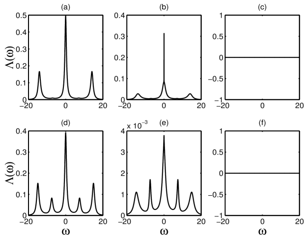
Figure 8: The fluorescence spectrum for the $V$-type three-level atom with non-degenerate transitions driven by a strong laser field of the Rabi frequency $\Omega=5\Gamma_{1}$, $\Delta_{L}=0,\Gamma_{1}=\Gamma_{2}=\Gamma$ and different $\Delta$ and $\Gamma_{12}$: (a) $\Delta=\Gamma,\Gamma_{12}=0$, (b) $\Delta=\Gamma,\Gamma_{12}=0.999\Gamma$, (c) $\Delta=\Gamma,\Gamma_{12}=\Gamma$, (d) $\Delta=5\Gamma,\Gamma_{12}=0$, (e) $\Delta=5\Gamma,\Gamma_{12}=0.999\Gamma$, (f) $\Delta=5\Gamma,\Gamma_{12}=\Gamma$.

We apply the equations of motion (89) to calculate numerically the steady-state fluorescence spectrum of the driven atom. In Fig. 8, we plot the fluorescence spectrum for a strong driving field tuned to the middle of the upper levels splitting $\Delta$. For small $\Delta$ the spectrum exhibits a three-peak structure, similar to the Mollow spectrum of a two-level atom [53], while for large $\Delta$ the spectrum consists of five peaks whose intensities and widths vary with the cross-damping term $\Gamma_{12}$. When the dipole moments are nearly parallel, $\Gamma_{12}=0.999\Gamma$, a significant sharp peak appears at the central frequency superimposed on a broad peak. However, in the case of exactly parallel dipole moments, $\Gamma_{12}=\Gamma$, and the fluorescence emission quenches completely at all frequencies.

The dependence of the number of peaks on the splitting $\Delta$, and the variation of their intensities and widths with $\Gamma_{12}$ can be readily explained in terms of transition rates between dressed states of the system. For the three-level system discussed here, the Hamiltonian is given by

$$H^{\prime}=H_{0}+V_{L},$$ (91)

where

$$H_{0}=-\hbar\left(\Delta_{L}-\frac{1}{2}\Delta\right)S_{1}^{+}S_{1}^{-}-\hbar\left(\Delta_{L}+\frac{1}{2}\Delta\right)S_{2}^{+}S_{2}^{-}+\hbar\omega_{L}a_{L}^{\dagger}a_{L}$$ (92)

is the Hamiltonian of the uncoupled system, and

$$V_{L}=-\frac{\hbar}{2}g\left[a_{L}^{\dagger}\left(S_{1}^{-}+S_{2}^{-}\right)+\left(S_{1}^{+}+S_{2}^{+}\right)a_{L}\right]$$ (93)

is the interaction between the laser field and the atomic transitions.

For $\Delta_{L}=0$ the Hamiltonian $H_{0}$ has three non-degenerate eigenstates $\left|2,N\right\rangle,$ $\left|1,N-1\right\rangle$, and $\left|3,N-1\right\rangle$, where $\left|i,N\right\rangle$ is the state with the atom in state $\left|i\right\rangle$ and $N$ photons present in the driving laser mode. When we include the interaction $V_{L}$ the triplets recombine into new triplets with eigenvectors (dressed states)

$$\left|+,N\right\rangle = \frac{1}{2}\left[\left(1-\alpha\right)\left|1,N-1\right\rangle+\left(1+\alpha\right)\left|3,N-1\right\rangle-2\beta\left|2,N\right\rangle\right],$$

$$\left|0,N\right\rangle = -\beta\left(\left|1,N-1\right\rangle-\left|3,N-1\right\rangle\right)+\alpha\left|2,N\right\rangle,$$ (94)

$$\left|-,N\right\rangle = \frac{-1}{2}\left[\left(1+\alpha\right)\left|1,N-1\right\rangle+\left(1-\alpha\right)\left|3,N-1\right\rangle+2\beta\left|2,N\right\rangle\right],$$

corresponding to energies

$$E_{N,+} = \hbar\left(N\omega_{L}+\tilde{\Omega}\right),$$

$$E_{N,0} = \hbar N\omega_{L},$$

$$E_{N,-} = \hbar\left(N\omega_{L}-\tilde{\Omega}\right),$$ (95)

where $\tilde{\Omega}=\sqrt{\Delta^{2}+\frac{1}{2}\Omega^{2}},\alpha=\Delta/2\tilde{\Omega}$ and $\beta=\Omega/2\tilde{\Omega}$.

The dressed states (94) group into manifolds, each containing three states. Neighbouring manifolds are separated by $\omega_{L}$, while the states inside each manifold are separated by $\tilde{\Omega}$. Interaction between the atom and the vacuum field leads to a spontaneous emission cascade down its energy manifold ladder. The probability of a transition between any two dressed states is proportional to the absolute square of the the dipole transition moment between these states. It is easily verified that non-zero dipole moments occur only between states within neighbouring manifolds. Using (94) and assuming that $\mbox{\boldmath$\mu$}_{13}=\mbox{\boldmath$\mu$}_{23}=\mbox{\boldmath$\mu$}$, we find that the transition dipole moments $\mbox{\boldmath$\mu$}_{i,N+1;0,N}=\left\langle N+1,i\right|\mbox{\boldmath$\mu$}\left|0,N\right\rangle$ between $\left|0,N\right\rangle$ and the dressed states of the manifold above are

$$\mbox{\boldmath$\mu$}_{+,N+1;0,N} = \frac{1}{2}\alpha\mbox{\boldmath$\mu$}\left[\left(1-\alpha\right)+\left(1+\alpha\right)\cos\theta\right],$$

$$\mbox{\boldmath$\mu$}_{0,N+1;0,N} = -\alpha\beta\mbox{\boldmath$\mu$}\left(1-\cos\theta\right),$$

$$\mbox{\boldmath$\mu$}_{-,N+1;0,N} = -\frac{1}{2}\alpha\mbox{\boldmath$\mu$}\left[\left(1+\alpha\right)+\left(1-\alpha\right)\cos\theta\right],$$ (96)

whereas the transition dipole moments between $\left|0,N\right\rangle$ and the dressed states of the manifold below are

$$\mbox{\boldmath$\mu$}_{0,N;+,N-1} = \beta^{2}\mbox{\boldmath$\mu$}\left(1-\cos\theta\right),$$

$$\mbox{\boldmath$\mu$}_{0,N;0,N-1} = -\alpha\beta\mbox{\boldmath$\mu$}\left(1-\cos\theta\right),$$

$$\mbox{\boldmath$\mu$}_{0,N;-,N-1} = \beta^{2}\mbox{\boldmath$\mu$}\left(1-\cos\theta\right),$$ (97)

where $\theta$ is the angle between the dipole moments.

It is apparent from Eq. (97) that transitions from the state $\left|0,N\right\rangle$ to the dressed states of the manifold below are allowed only if the dipole moments are not parallel. The transitions occur with significantly reduced rates, proportional to $(1-\cos\theta)$, giving very narrow lines when $\theta\approx 0^{o}$. For parallel dipole moments, the transitions to the state $\left|0,N\right\rangle$ are allowed from the dressed states of the manifold above, but are forbidden to the states of the manifold below. Therefore, the state $\left|0,N\right\rangle$ is a trapping state such that the population can flow into this state but cannot leave it, resulting in the disappearance of the fluorescence from the driven atom. The non-zero transition rates to the state $\left|0,N\right\rangle$ are proportional to $\alpha$ and are allowed only when $\Delta\neq 0$. Otherwise, for $\Delta=0$, the state $\left|0,N\right\rangle$ is completely decoupled from the remaining dressed states. In this case the three-level system is equivalent to a two-level atom.

The above dressed-atom analysis shows that quantum interference and the driving laser field create a “dressed” trapping state which is a linear superposition of the $|{a}\rangle$ and $|{2}\rangle$ states. This trapping state is different from the trapping state created by quantum interference in the absence of the driving field, see Eq. (62), which is the antisymmetric state $|{a}\rangle$ alone. As seen from Eq. (94), the dressed trapping state reduces to the state $|{a}\rangle$ for a very strong driving field $(\Omega\gg\Delta)$.

The narrow resonances produced by quantum interference may also be observed in the absorption spectrum of a three-level atom probed by a weak field of the frequency $\omega_{p}$. Zhou and Swain [13] have calculated the absorption spectrum of a probe field monitoring $V$-type three-level atoms with degenerate $(\Delta=0)$ as well as non-degenerate $(\Delta\neq 0)$ transitions and have demonstrated that quantum interference between the two atomic transitions can result in very narrow spectral lines, transparency, and even gain without population inversion. Paspalakis et al. [54] have calculated the absorption spectrum and refractive index of a $V$-type three-level atom driven by coherent and incoherent fields and have found that quantum interference enhances the index of refraction and can produce a very strong gain without population inversion.

7.4 Three-level $\Lambda$ system

It has been known for a long time, that in a $\Lambda$-type three-level atom with two transitions with perpendicular dipole moments $(\Gamma_{12}=0)$ driven by two laser fields, the population can be trapped in the ground states of the atom. This phenomenon, known as coherent population trapping (CPT) has been theoretically investigated by Arimondo and Orriols [55], Gray et al. [56], Orriols [57], and experimentally observed by Alzeta et al. [58]. Coherent population trapping has been examined in review articles by Dalton and Knight [59] and Arimondo  [60]. Javanainen [61], Ferguson et al. [62] and Menon and Agarwal [47] have examined the effect of quantum interference between the atomic transitions on the CPT and have demonstrated that the CPT effect strongly depends on the cross-damping term $\Gamma_{12}$ and disappears when $\Gamma_{12}=\Gamma$.

The CPT effect and its dependence on quantum interference can be easily explained by examining the population dynamics in terms of the superposition states $|{s}\rangle$ and $|{a}\rangle$. We assume that a three-level $\Lambda$-type atom is composed of a single upper state $\left|3\right\rangle$ and two ground states $\left|1\right\rangle$ and $\left|2\right\rangle$, and that the upper state is connected to the lower states by transition dipole moments $\mbox{\boldmath$\mu$}_{31}$ and $\mbox{\boldmath$\mu$}_{32}$.

Introducing superposition operators $S_{s}^{+}=\left(S_{s}^{-}\right)^{\dagger}=\left|3\right\rangle\left\langle s\right|$ and $S_{a}^{+}=\left(S_{a}^{-}\right)^{\dagger}=\left|3\right\rangle\left\langle a\right|$, where $\left|s\right\rangle$ and $\left|a\right\rangle$ are the superposition states

$$|{s}\rangle = \frac{1}{\sqrt{\Gamma_{1}+\Gamma_{2}}}\left(\sqrt{\Gamma_{1}}|{1}\rangle+\sqrt{\Gamma_{2}}|{3}\rangle\right),$$

$$|{a}\rangle = \frac{1}{\sqrt{\Gamma_{1}+\Gamma_{2}}}\left(\sqrt{\Gamma_{2}}|{1}\rangle-\sqrt{\Gamma_{1}}|{3}\rangle\right),$$ (98)

then, in the basis of the superposition states (98) the Hamiltonian of the system can be written as

$$H^{\prime} = -\hbar\left\{\left(\Delta_{L}-\frac{1}{2}\Delta^{\prime}\right)S_{s}^{-}S_{s}^{+}+\left(\Delta_{L}+\frac{1}{2}\Delta^{\prime}\right)S_{a}^{-}S_{a}^{+}\right.$$ (99)

$$+\left.\Delta_{c}\left(S_{s}^{-}S_{a}^{+}+S_{a}^{-}S_{s}^{+}\right)+\frac{1}{2}\frac{\sqrt{\Gamma_{1}}\Omega}{\sqrt{\Gamma_{1}+\Gamma_{2}}}\left(S_{s}^{+}+S_{s}^{-}\right)\right\},$$

where

$$\Delta^{\prime}=\frac{1}{\Gamma_{1}+\Gamma_{2}}\left[\left(\Gamma_{1}-\Gamma_{2}\right)\Delta+4\delta_{12}\sqrt{\Gamma_{1}\Gamma_{2}}\right].$$ (100)

and

$$\Delta_{c}=\frac{1}{\Gamma_{1}+\Gamma_{2}}\left[\delta_{12}\left(\Gamma_{1}-\Gamma_{2}\right)-\Delta\sqrt{\Gamma_{1}\Gamma_{2}}\right].$$ (101)

As before, $\Delta=\omega_{1}-\omega_{2}$, $\Delta_{L}=\omega_{L}-\frac{1}{2}\left(\omega_{1}+\omega_{2}\right)$, and we have assumed that $\Omega_{1}=\Omega_{2}=\Omega$.

From the master equation (29) with the Hamiltonian (99), we derive the following equation of motion for the population $\rho_{aa}$ of the antisymmetric state

$$\dot{\rho}_{aa}=\frac{2\Gamma_{1}\Gamma_{2}}{\Gamma_{1}+\Gamma_{2}}\left(1-p\right)\rho_{33}-i\Delta_{c}\left(\rho_{as}-\rho_{sa}\right).$$ (102)

The equation of motion (102) allows us to analyze the conditions for population trapping in the driven $\Lambda$ system. In the steady-state $(\dot{\rho}_{aa}=0)$ with $p\neq 1$ and $\Delta_{c}=0$ the population in the upper state is zero: $\rho_{33}=0$. Thus the state $\left|3\right\rangle$ is not populated despite the fact that it is continuously driven by the laser. In this case the population is entirely trapped in the antisymmetric superposition of the ground states. This is the coherent population trapping effect. However, for $p=1$ and $\Delta_{c}=0$ the antisymmetrical state decouples from the interactions, and then the steady-state population $\rho_{33}$ is non-zero [61]. This shows that coherent population trapping is possible only in the presence of spontaneous emission from the upper state to the antisymmetric superposition state. Thus, we can conclude that quantum interference has a destructive effect on coherent population trapping. Menon and Agarwal [47] have shown that the CPT effect can be preserved in the presence of quantum interference provided that the atom is driven by two coherent fields, each coupled to only one of the atomic transitions.

Figure 9: The stationary population of the upper state $\left|3\right\rangle$ of a $\Lambda$-type atom as a function of the splitting $\Delta$ for $\Delta_{L}=0,\Omega=5\Gamma_{1},\delta_{12}=0.1\Gamma_{1},p=0.5$ and different $\Gamma_{2}$: $\Gamma_{2}=\Gamma_{1}$ (solid line), $\Gamma_{1}=50\Gamma_{2}$ (dashed line).

According to Eq. (102) the CPT can also be destroyed by the presence of the coherent interaction $\Delta_{c}$ between the symmetric and antisymmetric states. This is shown in Fig. 9, where we plot the steady-state population $\rho_{33}$ as a function of $\Delta$ for different values of $\Gamma_{2}/\Gamma_{1}$. It is evident that the cancellation of the population $\rho_{33}$ appears only at $\Delta_{c}=0$, i.e. in the absence of the coherent interaction between the antisymmetric and symmetric states. For $\Gamma_{1}=\Gamma_{2}$ the cancellation appears at $\Delta=0$, while for $\Gamma_{1}\neq\Gamma_{2}$ the effect shifts towards non-zero $\Delta$ given by

$$\Delta=\frac{\Gamma_{1}-\Gamma_{2}}{\sqrt{\Gamma_{1}\Gamma_{2}}}\delta_{12}.$$ (103)

The shift depends on the ratio $r$, and for either $r\ll 1$ or $r\gg 1$ can be large despite $\delta_{12}$ being very small. Therefore, the vacuum induced coherent coupling can be experimentally observed in the $\Lambda$ system as a shift of the zero of the population $\rho_{33}$ of the upper state [32].

We have shown in Section 6.1 that a laser field can drive the $V$-type system into the antisymmetric (trapping) state through the coherent interaction between the symmetric and antisymmetric states. Recently, Akram et al. [32] have shown that in the $\Lambda$ system there are no trapping states to which the population can be transferred by the laser field. This can be illustrated by calculating the transition dipole moments between the dressed states of the driven $\Lambda$ system. The procedure of calculating the dressed states of the $\Lambda$ system is the same as for the $V$ system. The only difference is that now the eigenstates of the unperturbed Hamiltonian $H_{0}$ are $\left|3,N-1\right\rangle,\left|1,N\right\rangle,\left|2,N\right\rangle$, and the dressed states are given by

$$\left|+,N\right\rangle = \frac{1}{\sqrt{2}}\left[-\alpha\left|a,N\right\rangle+\left|s,N\right\rangle-\sqrt{2}\beta\left|3,N-1\right\rangle\right],$$

$$\left|0,N\right\rangle = -\sqrt{2}\beta\left|a,N\right\rangle+\alpha\left|3,N-1\right\rangle,$$

$$\left|-,N\right\rangle = \frac{1}{\sqrt{2}}\left[-\alpha\left|a,N\right\rangle-\left|s,N\right\rangle-\sqrt{2}\beta\left|3,N-1\right\rangle\right].$$ (104)

Although the dressed states (104) are similar to that of the $V$ system (see Eq. (94)), there is a crucial difference between the transition dipole moments. For the $\Lambda$ system the transition dipole moments between the dressed states $\left|i,N+1\right\rangle$ and the state $\left|0,N\right\rangle$ of the manifold below are all zero, but there are non-zero transition dipole moments between $\left|0,N\right\rangle$ and the dressed states $\left|i,N-1\right\rangle$ of the manifold below

$$\left\langle N,0\right|\mbox{\boldmath$\mu$}\left|\pm,N-1\right\rangle = \pm\alpha\mbox{\boldmath$\mu$},$$

$$\left\langle N,0\right|\mbox{\boldmath$\mu$}\left|0,N-1\right\rangle = 0.$$ (105)

Therefore, population is unable to flow into the state $\left|0,N\right\rangle$, but can flow away from it. If $\Delta=0$ then $\alpha=0$, and the state $\left|0,N\right\rangle$ completely decouples from the remaining states. For $\Delta\neq 0$ the state $\left|0,N\right\rangle$ is coupled to the remaining states, but does not participate in the dynamics of the system because it cannot be populated by transitions from the other states. Thus, there is no trapping state among the dressed states of the driven $\Lambda$ system.

8 Summary

In this paper we have discussed quantum interference effects in optical beams and radiation fields emitted from atomic systems. We have illustrated the effects using the first- and second-order correlation functions of optical fields and atomic dipole moments. We have explored the role of the correlations between radiating systems and have presented examples of practical methods to implement two systems with non-orthogonal dipole moments. Moreover, we have derived general conditions for quantum interference in a two-atom system and for control of spontaneous emission. We have shown that the cancellation of spontaneous emission does not necessarily lead to population trapping. The population can be trapped in a dark state only if the state is completely decoupled from any interactions. Finally, we have presented quantum dressed-atom models of cancellation of spontaneous emission, amplification on dark transitions, fluorescence quenching, and coherent population trapping.

Acknowledgments
This work was supported by the United Kingdom Engineering and Physical Sciences Research Council and the Australian Research Council. We wish to thank Helen Freedhoff, Paul Berman, Peng Zhou, Terry Rudolph, Howard Wiseman, Uzma Akram, and Jin Wang for many helpful discussions on quantum interference.

References

- [1] Mandel, L., and Wolf, E., 1995, Optical Coherence and Quantum Optics, (Cambridge, New York).
- [2] Dirac, P.A.M., 1981, The Principles of Quantum Mechanics, (Qxford University Press, Oxford).
- [3] Scully, M.O., and Zubairy, M.S., 1997 Quantum Optics, (Cambridge, New York).
- [4] Agarwal, G.S., 1974, Quantum Statistical Theories of Spontaneous Emission and their Relation to other Approaches, edited by Höhler, G., Springer Tracts in Modern Physics, Vol. 70, (Springer-Verlag , Berlin).
- [5] Zhou, P., and Swain, S., 1996, Phys. Rev. Lett. 77, 3995; 1997, Phys. Rev. A 56, 3011.
- [6] Keitel, C.H., 1999, Phys. Rev. Lett. 83, 1307.
- [7] Boller, K.J., Imamoglu, A., and Harris, S.E., 1991, Phys. Rev. Lett. 66, 2593; Hakuta, K., Marmet, L., and Stoicheff, B., 1991, Phys. Rev. Lett. 66, 596; Petch, J.C., Keitel, C.H., Knight, P.L., and Marangos,J.P., 1996, Phys. Rev. A 53, 543; Li, Y.-O., and Xiao, M., 1995, Phys. Rev. A 51, R2703, 4959.
- [8] For a recent review, see Mompart J. and Corbalan R. ,2000, J. Opt. B.: Qu and Semiclass. Opt., 2, R7.
- [9] Harris, S.E., 1989, Phys. Rev. Lett. 62, 1033; Scully, M.O., Zhu, S.-Y., and Gavrielides, A., 1989, Phys. Rev. Lett. 62, 2813; Agarwal, G.S., 1991, Phys. Rev. A 44, R28; Luo Z.-F., and Xu, Z.-Z., 1992, Phys. Rev. A 45, 8292; Tan, W., Lu, W., and Harrison, R.G., 1992, Phys. Rev. A 46, R3613; Keitel, C.H., Kocharovskaya, O., Narducci, L.M., Scully, M.O., Zhu, S.-Y., and Doss, H.M., 1993, Phys. Rev. A 48, 3196; Gawlik, W., 1993, Comments At. Mol. Phys. 29, 189; Grynberg, G., Pinard, M., and Mandel, P., 1996, Phys. Rev. A 54, 776; Kitching, J., and Hollberg, L., 1999, Phys. Rev. A 59, 4685.
- [10] Scully, M.O., 1991, Phys. Rev. Lett. 67, 1855; Scully, M.O., and Fleischhauer, M., 1992, Phys. Rev. Lett. 69, 1360; Wilson-Gordon, A.D., and Friedmann, H., 1992, Optics Commun. 94, 238; Quang, T., and Freedhoff, H., 1993, Phys. Rev. A 48, 3216; Akram, U., Wahiddin, M.R.B., and Ficek, Z., 1998, Phys. Lett. A238, 117.
- [11] Hau, L.V., Harris, S.E., Dutton, Z., and Behroozi, C.H., 1999, Nature 397, 594; Kash, M., Sautenkov, V., Zibrov, A., Hollberg, L., Welch, G., Lukin, M., Rostovtsev, Y., Fry, E., and Scully, M.O., 1999, Phys. Rev. Lett. 82, 5229; Lukin, M.D., and Imamoglu, A., 2000, Phys. Rev. Lett. 84, 1419.
- [12] E. Paspalakis and Knight, P. L., 1998, Phys. Rev. Lett., 81, 293; Petrosyan D. and Lambropoulos P., 2000, Phys. Rev. Lett., 85, 1843.
- [13] Zhou, P., and Swain, S., 1997, Phys. Rev. Lett. 78, 832.
- [14] Hegerfeldt, G.C., and Plenio, M.B., 1992, Phys. Rev. A 46, 373; Zhu, S.-Y., Chan, R.C.F., and Lee, C.P., 1995, Phys. Rev. A 52, 710; Toor, A.H., Zhu, S.-Y., and Zubairy, M.S., 1995, Phys. Rev. A 52, 4803; Plenio, M.B., and Knight, P.L., 1998, Rev. Mod. Phys. 70, 101; Li, F.-L., and Zhu, S.-Y., 1999, Phys. Rev. A 59, 2330; Lukin, M.D., Yelin, S.F., Fleischhauer, M., and Scully, M.O., 1999, Phys. Rev. A 60, 3225; Plastina, F., and Piperno, F., 2000, Phys. Rev. A 62, 053801.
- [15] Dicke, R.H., 1954, Phys. Rev. 93, 99; Milonni, P.W., and Knight, P.L., 1974, Phys. Rev. A 10, 1090; Freedhoff, H.S., 1986, J. Phys. B 19, 3035; Ficek, Z., Tanaś, R., and Kielich, S., 1987, Physica 146A, 452; Yang, G.J., Zobay, O., and Meystre, P., 1999, Phys. Rev. A 59, 4012; Beige, A., and Hegerfeldt, G.C., 1999, Phys. Rev. A 59, 2385.
- [16] Xia, H.R., Ye, C.Y., and Zhu, S.-Y., 1996, Phys. Rev. Lett. 77, 1032.
- [17] K. Hakuta, L. Marmet and B. P. Stoicheff, Phys. Rev. Lett. 66, 596 (1991).
- [18] Li, L., Wang, X., Jang, J., Lazarov, G., Qi, J., and Lyyra, A.M., 2000, Phys. Rev. Lett. 84, 4016.
- [19] Agarwal, G.S., 1997, Phys. Rev. A 55, 2457.
- [20] Berman, P.R., 1998, Phys. Rev. A 58, 4886.
- [21] Wang, J., Wiseman, H.M., and Ficek, Z., 2000, Phys. Rev. A 61, 063811.
- [22] Ryff, L.C., 1995, Phys. Rev. A 52, 2591; Englert, B.-G., 1996, Phys. Rev. Lett. 77, 2154.
- [23] Hanbury-Brown, R., and Twiss, R.Q., 1956, Nature 177, 27.
- [24] Javan, A., Ballik, E.A., and Bond, W.L., 1962, J. Opt. Soc. Am. 52, 96; Lipsett, M.S., and Mandel, L., 1963, Nature 199, 553.
- [25] Glauber, R. J., 1965, in “Quantum Optics and Electronics”, eds. C. DeWitt et al., Gordon and Breach.
- [26] Richter, Th., 1979, Ann. Phys. (Leipzig) 36, 266; Mandel, L., 1983, Phys. Rev. A 28, 1929; Gosh, R., Hong, C.K., Ou, Z.Y., and Mandel, L., 1986, Phys. Rev. A 34, 3962; Ficek, Z., Tanaś, R., and Kielich, S., 1998, J. Mod. Opt. 35, 81.
- [27] Walls, D.F., and Milburn, G.J., 1994, Quantum Optics, (Springer, Berlin).
- [28] Gosh, R., and Mandel, L., 1987, Phys. Rev. Lett. 59, 1903; Hong, C.K., Ou, Z.Y., and Mandel, L., 1987, Phys. Rev. Lett. 59, 2044; Ou, Z.Y., and Mandel, L., 1989, Phys. Rev. Lett. 62, 2941.
- [29] Richter, Th., 1990, Phys. Rev. A 42, 1817.
- [30] Lehmberg, R.H., 1970, Phys. Rev. A 2, 883.
- [31] Cardimona, D.A., and Stroud, C.R., Jr., 1983, Phys. Rev. A 27, 2456.
- [32] Akram, U., Ficek, Z., and Swain, S., 2000, Phys. Rev. A 62, 013413.
- [33] Ficek, Z., and Freedhoff, H.S., 1996, Phys. Rev. A 53, 4275; Rudolph, T., Freedhoff, H.S., and Ficek, Z., 1998, J. Opt. Soc. Am. B 15, 2345; Yu, C.C., Bochinski, J.R., Kordich, T.M.V., Mossberg, T.W., and Ficek, Z., 1997, Phys. Rev. A 56, R4381; Ficek, Z., and Rudolph, T., 1999, Phys. Rev. A 60, R4245.
- [34] Cohen-Tannoudji, C., and Reynaud, S., 1977, J. Phys. B 10, 345; Cohen-Tannoudji, C., Dupont-Roc, J., and Grynberg, G., 1992, Atom-Photon Interactions (Wiley, New York).
- [35] Patnaik, A.K., and Agarwal, G.S., 1999, Phys. Rev. A 59, 3015.
- [36] Zhou, P., and Swain, S., 2000, Optics Commun. 179, 267; Zhou, P., Swain, S., and You L., 2001, Phys Rev. A, 63, 033818.
- [37] Zhou, P., 2000, Optics Commun. 178, 141.
- [38] Agarwal, G.S., 2000, Phys. Rev. Lett. 84, 5500.
- [39] Eichmann, U., Bergquist, J.C., Bollinger, J.J., Gilligan, J.M., Itano, W.M., Wineland, D.J., and Raizen, M.G., 1993, Phys. Rev. Lett. 70, 2359.
- [40] Ficek, Z., Tanaś, R., and Kielich, S., 1987, Physica 146A, 452; Ficek, Z., and Tanaś, R., 1998, Optics Commun. 153, 245.
- [41] Dung, H.T., and Ujihara, K., 2000, Phys. Rev. Lett. 84, 254; Richter, Th., 1991, Optics Commun. 80, 285; Hegerfeldt, G.C., and Plenio, M.B., 1993, Phys. Rev. A 47, 2186.
- [42] Ficek, Z., and Sanders, B.C., 1990, Phys. Rev. A 41, 359; Rudolph, T.G., Ficek, Z., and Dalton, B.J., 1995, Phys. Rev. A 52, 636; Rudolph, T., and Ficek, Z., 1998, Phys. Rev. A 58, 748; Skornia, C., von Zanthier, J., Agarwal, G.S., Werner, E., and Walther, H., quant-ph/0103031.
- [43] Bužek, V., Knight, P.L., and Kudryavtsev, I.K., 1991, Phys. Rev. A 44, 1931.
- [44] Zhu, S.-Y., and Scully, M.O., 1996, Phys. Rev. Lett. 76, 388.
- [45] Lax, M., 1968, Phys. Rev. 172, 350.
- [46] Lee, H., Polynkin, P., Scully, M.O.,and Zhu, S.-Y., 1997, Phys. Rev. A 55, 4454.
- [47] Menon, S., and Agarwal, G.S., 1998, Phys. Rev. A 57, 4014.
- [48] Akram, U., Ficek, Z., and Swain, S., 2001, J. Mod. Opt. (in press).
- [49] Menon, S., and Agarwal, G.S., 2000, Phys. Rev. A 61, 013807.
- [50] Mollow, B.R., 1972, Phys. Rev. A 5, 1522, 2217.
- [51] Ficek, Z., Swain, S., and Akram, U., 2001, J. Phys. B 34, 671.
- [52] Cardimona, D.A., Raymer, M.G., and Stroud, C.R., Jr., 1982, J. Phys. B 15, 55.
- [53] Mollow, B.R., 1969, Phys. Rev. 188, 1969.
- [54] Paspalakis, E., and Knight, P.L., 1998, Phys. Rev. Lett. 81, 293; Paspalakis, E., Gong, S.-Q., and Knight, P.L., 1998, Optics Commun. 152, 293.
- [55] Arimondo, E., and Orriols, G., 1976, Lett. Nuovo Cimento 17, 333.
- [56] Gray, H.R., Whitley, R.M., and Stroud, C.R., Jr., 1978, Opt. Lett. 3, 218.
- [57] Orriols, G., 1979, Nuovo Cimento B 53, 1.
- [58] Alzetta, G., Gozzini, A., Moi, L., and Orriols, G., 1976, Nuovo Cimento B 36, 5.
- [59] Dalton, B.J., and Knight, P.L., 1983, in: Laser Physics, Lecture Notes in Physics, Vol. 182, eds. J.D. Harvey and D.F. Walls (Springer, Berlin), p. 213.
- [60] Arimondo, E., 1996, Progress in Optics XXXV, edited by E. Wolf (Elsevier, Amsterdam), p. 257.
- [61] Javanainen, J., 1992, Europhys. Lett. 17, 407.
- [62] Ferguson, M.R., Ficek, Z., and Dalton, B.J., 1995, J. Mod. Opt. 42, 679.