Quantum machine language and quantum computation with Josephson junctions

Abstract

An implementation method of a gate in a quantum computer is studied in terms of a finite number of steps evolving in time according to a finite number of basic Hamiltonians, which are controlled by on-off switches. As a working example, the case of a particular implementation of the two qubit computer employing a simple system of two coupled Josephson junctions is considered. The binary values of the switches together with the time durations of the steps constitute the quantum machine language of the system.

I Introduction

In classical computing the programming is based on commands written in the machine language. Each command is translated into manipulations of the considered device, obtained by electronic switches. In quantum computation quantum mechanics is employed to process information. Therefore the conception of the quantum computer programming, the structure of the quantum machine language and the commands are expected to be quite different from the classical case. Although there are differences between classical and quantum computers, the programming in both cases should be based on commands, and a part of these commands is realized by quantum gates. Initially, one of the leading ideas in quantum computation was the introduction of the notion of the universal gate DeuPRSL85 . Given the notion of a universal set of elementary gates, various physical implementations of a quantum computer have been proposed BraLoFDP00 . Naturally, in order for an implementation to qualify as a valid quantum computer, all the set of elementary gates have to be implemented by the proposed system. This property is related to the problem of controllability of the quantum computer.The controllability of quantum systems is an open problem under investigation RaViMoKo00 . Recently, DiVincpre01 ; DiVincNa00 attention was focused on the notion of encoded universality, which is a different functional approach to the quantum computation. Instead of forcing a physical system to act as a predetermined set of universal gates, which will be connected by quantum connections, the focus of research is proposed to be shifted to the study of the intrinsic ability of a given physical system, to act as a quantum computer using only its natural available interactions. Therefore the quantum computers are rather a collection of interacting cells (e.g. quantum dots, nuclear spins, Josephson junctions etc). These cells are controlled by external classical switches and they evolve in time by modifying the switches. The quantum algorithms are translated into time manipulations of the external classical switches which control the system. This kind of quantum computer does not have connections, which is the difficult part of a physical implementation. Any device operating by external classical switches has an internal range of capabilities, i.e. it can manipulate the quantum information encoded in a subspace of the full system of Hilbert space. This capability is called encoded universality of the system DiVincpre01 . The notion of the encoded universality is identical to the notion of the controllability RaViMoKo00 of the considered quantum device. The controllability on Lie groups from a mathematical point of view was studied in JurSus75 ; Rama95 ; Rama01 ; KhaGla01 ; FuSchSo01 . The controllability of atomic and molecular systems was studied by several authors see review article RaViMoKo00 and the special issue of the Chemical Physics vol. 267, devoted to this problem. In the case of laser systems the question of controllability was studied by several authors and recently in FuSchSo01 ; SchFuSo01 . In the present paper we investigate the conditions in order to obtain the full system of Hilbert space by a finite number of choices of the values of the classical switches. As a working example we use the Josephson junction devices in their simplest form NakaPRL97 ; AveSSC98 ; AveNa99 ; ShnSchPRL97 , but this study can be extended in the case of quantum dots or NMR devices.

In this paper the intrinsic interaction of a system operating as a universal computer is employed instead of forcing the system to enact a predetermined set of universal gates DiVincpre01 . As a basic building block we use a system of two identical Josephson junctions coupled by a mutual inductor. The values of the classical control parameters (the charging energy $E_{c}$ and the inductor energy $E_{L}$) are chosen in such a way that four basic Hamiltonians, $H_{i}$,($i=1,\ldots,4$) are created by switching on and off the bias voltages and the inductor, where the tunneling amplitude $E_{J}$ is assumed to be fixed. Our procedure allows the construction of any one-qubit and two-qubit gate, through a finite number of steps evolving in time according to the four basic Hamiltonians. Using the two Josephson junctions network a construction scheme of four steps for the simulation is presented in the case of an arbitrary one-qubit gate, and of fifteen steps, for the simulation of an arbitrary two-qubit gate. The main idea of this paper is the use of a small number of Hamiltonian states in order to obtain the gates.

Our results can be formulated in terms of a quantum machine language. For example, each two-qubit gate $U$ is represented by a command of the language containing 15 letters i.e. the fifteen steps mentioned above. Each letter consists of a binary part (the states of the on-off switches), which determines the basic Hamiltonian used, and a numerical part corresponding to the time interval.

Our proposal can be generalized for $N$-qubit gates ($N>2$) belonging to the $SU(2^{N})$. In that case $N+2$ basic Hamiltonians are needed to implement such a gate. The generalization of these ideas is under investigation.

The paper is organized as follows: In section II we present for clarity reasons the formalism of Josephson junctions one-qubit devices. In section III we apply the formalism to two qubit gates and simulate two-qubit gates and the possible $N$-qubit generalizations are discussed. In section IV the results are summarized. Finally in the Appendix A, the essential mathematical feedback is provided.

II One-qubit devices

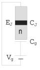
Figure 1: One qubit device

The simplest Josephson junction one qubit device is shown in Fig 1. In this section we give a summary of the considered device. The detailed description and the complete list of references can be found in the detailed review paper (MahkRMP00, , section II). The device consists of a small superconducting island (”box”), with $n$ excess Cooper pair charges connected by a tunnel junction with capacitance $C_{J}$ and Josephson coupling energy $E_{J}$ to a superconducting electrode. A control gate voltage $V_{g}$ (ideal voltage source) is coupled to the system via a gate capacitor $C_{g}$.

The chosen material is such that the superconducting energy gap is the largest energy in the problem, larger even than the single-electron charging energy. In this case quasi-particle tunneling is suppressed at low temperatures, and a situation can be reached where no quasi-particle excitation is found on the island. Under special condition described in ref MahkRMP00 only Cooper pairs tunnel coherently in the superconducting junction.

The voltage $V_{g}$ is constrained in a range interval where the number of Cooper pairs takes the values $0$ and $1$, while all other coherent charge states, having much higher energy, can be ignored. These charge states correspond to the spin basis states:
$|\uparrow>$ corresponding to $0$ Cooper-pair charges on the island, and $|\downarrow>$ corresponding to $1$ Cooper-pair charges.
In this case the superconducting charge box reduces to a two-state quantum system, qubit, with Hamiltonian (in spin 1/2 notation):

$$\begin{array}[]{c}H=\frac{1}{2}E_{c}\,\sigma_{z}-\frac{1}{2}E_{J}\,\sigma_{x},\quad\sigma_{z}|\uparrow>=|\uparrow>\quad\mbox{and}\\ \quad\sigma_{z}|\downarrow>=-|\downarrow>.\end{array}$$ (1)

In this Hamiltonian there are two parameters the bias energy $E_{c}$ and the tunneling amplitude $E_{J}$. The bias energy $E_{c}$ is controlled by the gate voltage $V_{g}$ of Fig 1, while the tunneling amplitude $E_{J}$ here is assumed to be constant i.e. it is a constant system parameter. The tunneling amplitude can be controlled in the case of the tunable effective Josephson junction, where the single Josephson junction is replaced by a flux-threaded SQUID MahkRMP00 , but this device is more complicated than the one considered in this paper.

The Hamiltonian is written as:

$$H=\frac{1}{2}\Delta E(\eta)(\cos\eta\,\sigma_{z}-\sin\eta\,\sigma_{x})$$ (2)

where $\eta$ is the mixing angle

$$\eta\equiv\tan^{-1}\frac{E_{J}}{E_{c}}$$

The energy eigenvalues are

$$E_{\pm}=\pm\frac{\Delta E(\eta)}{2}$$

and the splitting between the eigenstates is:

$$\Delta E(\eta)=\sqrt{E_{J}^{2}+E_{c}^{2}}$$

The eigenstates provided by the Hamiltonian (1), are denoted in the following as $|+>$ and $|->$:

$$\begin{array}[]{rl}|+>&=\cos{\frac{\eta}{2}}\,|\downarrow>+\sin{\frac{\eta}{2}}\,|\uparrow>\\ |->&=\sin{\frac{\eta}{2}}\,|\downarrow>-\cos{\frac{\eta}{2}}\,|\uparrow>\end{array}$$ (3)

To avoid confusion we introduce a second set of Pauli matrices $\vec{\rho}=(\rho_{x},\rho_{y},\rho_{z})$, which operate in the basis $|+>$, $|->$, while reserving the $\vec{\sigma}$ operators for the basis of $|\uparrow>$ and $|\downarrow>$:

$$\begin{array}[]{c}\rho_{z}=|+><+|\,-\,|-><-|,\\ \rho_{x}=|+><-|\,+\,|-><+|,\\ \rho_{y}=i|-><+|\,-\,i|+><-|\end{array}$$

In the proposed model we assume that the device of Fig 1 has a switch taking two values $1$ and $0$, corresponding to the switch states ON and OFF. This switch controls the gate voltage $V_{g}$, which takes only two values either $V_{\rm id}$ or $V_{\rm deg}$, where the first one corresponds to the idle Hamiltonian, while the second one corresponds to the degenerate Hamiltonian.

The idle point can be achieved for a characteristic value of the control gate voltage $V_{g}=V_{\rm id}$, corresponding to a special value of the bias energy and to the phase parameter $\eta=\eta_{\rm id}$. At this point the energy splitting $\Delta E(\eta)$ achieves its maximum value, which is denoted by $\Delta E$. For simplicity reasons we reserve the symbol $E_{c}$ for the bias energy corresponding to the idle point and by definition, the Hamiltonian at the idle point then becomes:

$$H_{\rm id}=\frac{E_{c}}{2}\sigma_{z}-\frac{E_{J}}{2}\sigma_{x}=\frac{1}{2}\Delta E\,\rho_{z}$$ (4)

At the degeneracy point $\eta=\frac{\pi}{2}$ the energy splitting reduces to $E_{J}$, which is the minimal energy splitting. This point is characteristic for the material of the Josephson junction and corresponds to a special characteristic choice of the control gate voltage $V_{g}=V_{\rm deg}$.

$$H_{\rm deg}=-\frac{E_{J}}{2}\sigma_{x}=-\frac{E_{J}}{2}\left(\sin\eta_{\rm id}\rho_{z}-\cos\eta_{\rm id}\rho_{x}\right)$$ (5)

The system is switched in the state OFF (or $0$) corresponding to the degenerate Hamiltonian (5) during a time interval $t_{1}$, then the system is switched to the state ON (or $1$) i.e. the idle Hamiltonian (4) during a time interval $t_{2}$ and it comes back to the initial degenerate Hamiltonian during the time $t_{3}$. The general form of the evolution operator is:

$$U={\rm e}^{-it_{3}H_{\rm deg}}\,{\rm e}^{-it_{2}H_{\rm id}}\,{\rm e}^{-it_{1}H_{\rm deg}}$$ (6)

The operators $H_{\rm id}$ and $H_{\rm deg}$ and their commutator

$$\left[H_{\rm id},H_{\rm deg}\right]=i\frac{E_{c}E_{J}}{2}\sigma_{y}$$

form a (non-orthogonal) basis of the algebra $su(2)$. Therefore the pair $H_{\rm id},\,H_{\rm deg}$ generates $su(2)$ by taking these elements and all their possible commutators and their linear combinations. That means that the combination of three terms as in equation (6) for all the triples $\{t_{1},t_{2},t_{3}\}$ cover all the matrices belonging in $SU(2)$. Thus we conclude that every 2$\times$2 matrix $U$ in $SU(2)$ can be achieved by a device as in Fig 1, with manipulation of the binary switch permitting to the Hamiltonian two possible states i.e. the idle one and the degenerate one. The above described manipulations can be codified by a rudimentary Quantum Machine Language (QML) for the one qubit device. In that elementary language the gate $U$ corresponds to a command of the language, each command is constituted by (three) letters, each of them having the form of a pair

$$\{e,t\},\quad e=0\,(OFF),\mbox{ or }1\,(ON),\mbox{ and }0\leq t<\infty$$

i.e. the command corresponding to equation (6) is analyzed in the following (at most three) letters:

$$\begin{array}[]{|c|}\hline\cr U\\ \hline\cr\hline\cr\{0,t_{1}\}\\ \hline\cr\{1,t_{2}\}\\ \hline\cr\{0,t_{3}\}\\ \hline\cr\end{array}$$

The one qubit gates are $2\times 2$ unitary matrices belonging to the group U(2). Each element in the group $U(2)$ can be projected up to one multiplication constant to an element of group $SU(2)$. Evidently the elements generated by the evolution operator (6) belong to $SU(2)$. Throughout this paper we shall use projections of $U(2^{N})$ matrices in $SU(2^{N})$, using the symbol “$\mapsto$” to denote this projection. Let us consider the fundamental one qubit gates or commands NOT, $\sqrt{\rm NOT}$, Hadamard, Phase Shift and their $SU(2)$ projections:

$${\rm NOT}=\left(\begin{array}[]{cc}0&1\\ 1&0\end{array}\right)\mapsto i\sigma_{x}={\rm e}^{-i\frac{\pi}{E_{J}}\,H_{\rm deg}}\in SU(2),$$

$$\begin{array}[]{rl}\sqrt{\rm NOT}=&\frac{1}{\sqrt{2}}\left(\begin{array}[]{cc}{\rm e}^{-i\frac{\pi}{4}}&{\rm e}^{i\frac{\pi}{4}}\\ {\rm e}^{i\frac{\pi}{4}}&{\rm e}^{-i\frac{\pi}{4}}\end{array}\right)\mapsto\\ &\mapsto\frac{1}{\sqrt{2}}\left(\,\mathbb{I}+i\sigma_{x}\right)={\rm e}^{-i\left(\frac{\pi}{2E_{J}}\right)\,H_{\rm deg}}\end{array}$$

$$\begin{array}[]{rl}{\rm Had}=&\frac{1}{\sqrt{2}}\left(\begin{array}[]{cc}1&1\\ 1&-1\end{array}\right)\mapsto\frac{i}{\sqrt{2}}\left(\sigma_{x}+\sigma_{z}\right)=\\ =&{\rm e}^{-it_{3}^{\rm h}H_{\rm deg}}\,{\rm e}^{-it_{2}^{\rm h}H_{\rm id}}\,{\rm e}^{-it_{1}^{\rm h}H_{\rm deg}}\end{array}$$

where

$$t_{1}^{\rm h}=t_{3}^{\rm h}=\frac{2\left(\cos^{-1}\left[\sqrt{\frac{E_{J}+E_{c}}{2E_{c}}}\;\right]+\frac{\pi}{2}\right)}{E_{J}},$$

$$t_{2}^{\rm h}=\frac{2\left(\sin^{-1}\left[{\frac{\Delta E}{\sqrt{2}E_{c}}}\right]+\pi\right)}{\Delta E}$$

$$\begin{array}[]{rl}{\rm PhS}=&\left(\begin{array}[]{cc}1&0\\ 0&{\rm e}^{i\phi}\end{array}\right)\mapsto\cos{\frac{\phi}{2}}\,\mathbb{I}-i\sin{\frac{\phi}{2}}\,\sigma_{z}=\\ =&{\rm e}^{-it_{3}^{\rm ph}H_{\rm deg}}\,{\rm e}^{-it_{2}^{\rm ph}H_{\rm id}}\,{\rm e}^{-it_{1}^{\rm ph}H_{\rm deg}}\end{array}$$

where

$$\begin{array}[]{rl}t_{1}^{\rm ph}=&t_{3}^{\rm ph}=\\ =&\frac{2\left(\cos^{-1}\left[\frac{1}{2}\sqrt{2-\frac{\sqrt{2}\,\Delta E\,\sqrt{-1+\frac{2E_{c}^{2}}{\Delta E^{2}}+\cos\phi}}{E_{c}\,\cos\frac{\phi}{2}}}\;\right]+\frac{\pi}{2}\right)}{E_{J}},\end{array}$$

$$t_{2}^{\rm ph}=\frac{2\left(\sin^{-1}\left[\frac{\Delta E\,\sin\frac{\phi}{2}}{E_{c}}\right]\right)}{\Delta E}$$

The above formulas imply the following analysis of these commands in letters (Table 1).

$$\begin{array}[]{cccc}\begin{array}[]{|c|}\hline\cr{\rm NOT}\\ \hline\cr\hline\cr\{0,\pi/E_{J}\}\\ \hline\cr--\\ \hline\cr--\\ \hline\cr\end{array}&\begin{array}[]{|c|}\hline\cr\sqrt{{\rm NOT}}\\ \hline\cr\hline\cr\{0,\pi/2E_{J}\}\\ \hline\cr--\\ \hline\cr--\\ \hline\cr\end{array}&\begin{array}[]{|c|}\hline\cr{\rm Had}\\ \hline\cr\hline\cr\{0,t_{1}^{\rm h}\}\\ \hline\cr\{1,t_{2}^{\rm h}\}\\ \hline\cr\{0,t_{3}^{\rm h}\}\\ \hline\cr\end{array}&\begin{array}[]{|c|}\hline\cr{\rm PhS}\\ \hline\cr\hline\cr\{0,t_{1}^{\rm ph}\}\\ \hline\cr\{1,t_{2}^{\rm ph}\}\\ \hline\cr\{0,t_{3}^{\rm ph}\}\\ \hline\cr\end{array}\end{array}$$

Table 1: Letter Analysis of One-qubit gates

The above analysis of a quantum gate in letters is rather trivial in the one qubit case and it was presented for clarity reasons, but the similar construction is far from evident and quite complicated in the $N$-qubit case.

III Two-qubit devices

In order to perform one and two qubit quantum gate manipulations in the same device, we need to couple pairs of qubits together and to control the interaction between them. For this purpose identical Josephson junctions are coupled by one mutual inductor $L$ as shown in Fig 2. The physics and the detailed description of the coupled Josephson junctions are discussed and reviewed in MahkRMP00 . For $L=0$ the system reduces to a series of uncoupled, single qubits, while for $L\rightarrow\infty$ they are coupled strongly. The ideal system would be one where the coupling between different qubits could be switched in the state ON (or state ${}^{\prime}1^{\prime}$) by applying an induction via a constant value inductor $L$ and in the state OFF (or state ${}^{\prime}0^{\prime}$) corresponding to $L=0$ and leaving the qubits uncoupled in the idle state.

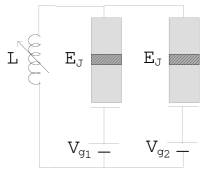
Figure 2: Two qubit device

The Hamiltonian for a general two-qubit system is written:

$$\begin{array}[]{rl}H=&H_{1}+H_{2}+H_{\rm int}=\\ =&{\frac{1}{2}}E_{c_{1}}\,\sigma_{z}^{(1)}-{\frac{1}{2}}E_{J_{1}}\,\sigma_{x}^{(1)}+\\ &+{\frac{1}{2}}E_{c_{2}}\,\sigma_{z}^{(2)}-{\frac{1}{2}}E_{J_{2}}\,\sigma_{x}^{(2)}-{\frac{1}{2}}E_{L}\,\sigma_{y}^{(1)}\,\sigma_{y}^{(2)}\end{array}$$ (7)

For an explanation of the formalism used in this section see Appendix A. In the case of two identical junctions we have $E_{J_{1}}=E_{J_{2}}=E_{J}$, since the tunneling amplitude of the junction is a system parameter, depending on the material. Under these conditions the two coupled Josephson junctions Hamiltonian will be controlled by the following control parameters : $E_{c_{1}},\,E_{c_{2}},\,E_{L}$, which will be called switches. The first two parameters are controlled by the gate voltages $V_{g_{1}},\,V_{g_{2}}$, while the last parameter is related to the inductor switch $L$. In the proposed model each of the parameters $E_{c_{1}},\,E_{c_{2}}$ can have two values $0$ or $E_{c}$. The first is the state ${}^{\prime}0^{\prime}$ (or $OFF$) corresponding to the degenerate one qubit state, while the other one is equal to $E_{c}$ (or $ON$ or ${}^{\prime}1^{\prime}$ state) corresponding to the one qubit idle state. Also the parameter $E_{L}$ takes two values. The one is $E_{L}=0$ ($OFF$ or ${}^{\prime}0^{\prime}$ state) corresponding to a an uncoupled two qubit state and the other one has a fixed value ($ON$ or ${}^{\prime}1^{\prime}$ state). For the sake of simplicity we use the symbol $E_{L}$ for this induction amplitude. Using this combination of parameter values or binary switches values, we can obtain the following four fundamental states of the Hamiltonian (7):

• where both of the junctions are in the idle state $(E_{c_{1}}=E_{c_{2}}=E_{c})$, while they are uncoupled $(E_{L}=0)$.

  $$H_{1}={\frac{1}{2}}E_{c}\,(\sigma_{z}^{(1)}+\sigma_{z}^{(2)})-{\frac{1}{2}}E_{J}\,(\sigma_{x}^{(1)}+\sigma_{x}^{(2)})$$ (8)

  This Hamiltonian corresponds to the switches choice $(E_{c_{1}},\,E_{c_{2}},\,E_{L})\rightarrow(1,1,0)$.

• where both of the junctions are in the degenerate state $(E_{c_{1}}=E_{c_{2}}=0)$, while the two qubits are coupled.

  $$H_{2}=-{\frac{1}{2}}E_{J}\,(\sigma_{x}^{(1)}+\sigma_{x}^{(2)})-{\frac{1}{2}}E_{L}\,\sigma_{y}^{(1)}\sigma_{y}^{(2)}$$ (9)

  corresponding to the switch choice $(0,0,1)$.

• where the first junction is in degeneracy $(E_{c_{1}}=0)$, the second is in the idle state $(E_{c_{2}}=E_{c})$ and they are uncoupled $(E_{L}=0)$.

  $$H_{3}={\frac{1}{2}}E_{c}\,\sigma_{z}^{(2)}-{\frac{1}{2}}E_{J}\,(\sigma_{x}^{(1)}+\sigma_{x}^{(2)})$$ (10)

  corresponding to the switch choice $(0,1,0)$.

• where the first junction is in the idle state $(E_{c_{1}}=E_{c})$, the second is in the degeneracy $(E_{c_{2}}=0)$ and they are uncoupled $(E_{L}=0)$.

  $$H_{4}={\frac{1}{2}}E_{c}\,\sigma_{z}^{(1)}-{\frac{1}{2}}E_{J}\,(\sigma_{x}^{(1)}+\sigma_{x}^{(2)})$$ (11)

  corresponding to the switch choice $(1,0,0)$.

These four Hamiltonian forms are linearly independent and they can generate the su$(4)$ algebra by repeated commutations and linear combinations. For a detailed discussion see the discussion in Appendix A, equation (25). From Proposition A.2, any elementary two-qubit gate, which is represented by a unitary $4\times 4$ matrix $U\in$SU$(4)$, can be constructed as follows:

$$\begin{array}[]{rl}U=&{\rm e}^{-iH_{3}t_{15}}{\rm e}^{-iH_{2}t_{14}}\cdots{\rm e}^{-iH_{2}t_{6}}\cdot\\ &\cdot{\rm e}^{-iH_{1}t_{5}}{\rm e}^{-iH_{4}t_{4}}{\rm e}^{-iH_{3}t_{3}}{\rm e}^{-iH_{2}t_{2}}{\rm e}^{-iH_{1}t_{1}}\end{array}$$ (12)

From a physical point of view any two qubit quantum gate can be obtained by 15 time steps. At the k-th step the device is put at one of the Hamiltonian states $H_{1},\ H_{2},\,H_{3}$ or $H_{4}$ by appropriate manipulations of the switches during a time interval $t_{k},\,k=1,2,\ldots,15$. Using this fact a Quantum Machine Language (QML) can be defined as in section II. Each gate, corresponding to the $4\times 4$ matrix $U$, is associated to a command of the QML. Each command consists of at most $15$ letters or steps, each of them being a collection of $4$ numbers $\{e_{1},\,e_{2},\,\ell,\,t\}$ of the following form:

$$\begin{array}[]{c}\mbox{\emph{letter}}\,\Leftrightarrow\,\{e_{1},\,e_{2},\,\ell,\,t\}\qquad 0\leq t<\infty\\ \begin{array}[]{rll}\hline\cr e_{1}=0&\mbox{ if }V_{g_{1}}=V_{\rm deg}&\;\Rightarrow\;E_{c_{1}}=0\\ =1&\mbox{ if }V_{g_{1}}=V_{\rm id}&\;\Rightarrow\;E_{c_{1}}=E_{c}\\ \hline\cr e_{2}=0&\mbox{ if }V_{g_{2}}=V_{\rm deg}&\;\Rightarrow\;E_{c_{2}}=0\\ =1&\mbox{ if }V_{g_{2}}=V_{\rm id}&\;\Rightarrow\;E_{c_{2}}=E_{c}\\ \hline\cr\ell=0&\mbox{ if }L=0&\;\Rightarrow\;E_{L}=0\\ =1&\mbox{ if }L\neq 0&\;\Rightarrow\;E_{L}\neq 0\\ \hline\cr\end{array}\end{array}$$

The gate $U$ given by equation (12) corresponds to one command, which contains $15$ letters and is presented in Table 2. Each letter is the codified command which indicates the state of the binary switches and the time interval.

$$\begin{array}[]{|c|}\hline\cr U\\ \hline\cr\hline\cr\{1,1,0,t_{1}\}\\ \hline\cr\{0,0,1,t_{2}\}\\ \hline\cr\{0,1,0,t_{3}\}\\ \hline\cr\{1,0,0,t_{4}\}\\ \hline\cr\{1,1,0,t_{5}\}\\ \hline\cr\{0,0,1,t_{6}\}\\ \hline\cr\{0,1,0,t_{7}\}\\ \hline\cr\{1,0,0,t_{8}\}\\ \hline\cr\{1,1,0,t_{9}\}\\ \hline\cr\{0,0,1,t_{10}\}\\ \hline\cr\{0,1,0,t_{11}\}\\ \hline\cr\{1,0,0,t_{12}\}\\ \hline\cr\{1,1,0,t_{13}\}\\ \hline\cr\{0,0,1,t_{14}\}\\ \hline\cr\{0,1,0,t_{15}\}\\ \hline\cr\end{array}$$

Table 2: Letter analysis of a command (gate) $U$

We should notice that the succession of switch states follows a cyclic pattern. This regularity might facilitate the manipulation of the coupled junction device.

Let us now give some numerical simulations of the proposed model for some fundamental quantum gates essential for the quantum computation (we use these gates multiplied with a proper constant because the corresponding matrices should be elements of the $SU(4)$ group) . These gates are :

1. The CNOT gate. Probably the most important gate in quantum computation:

   $$\begin{array}[]{cl}{\rm CNOT}&=\left(\begin{array}[]{cccc}1&0&0&0\\ 0&1&0&0\\ 0&0&0&1\\ 0&0&1&0\end{array}\right)\mapsto\\ \\ &\mapsto\frac{{\rm e}^{i\frac{\pi}{4}}}{2}\,(-\sigma_{z}^{(1)}\sigma_{x}^{(2)}+\sigma_{z}^{(1)}+\sigma_{x}^{(2)}+\mathbb{I}\otimes\mathbb{I})\in SU(4)\end{array}$$

2. The SWAP gate, which interchanges the input qubits:

   $$\begin{array}[]{cl}{\rm SWAP}&=\left(\begin{array}[]{cccc}1&0&0&0\\ 0&0&1&0\\ 0&1&0&0\\ 0&0&0&1\end{array}\right)\mapsto\\ \\ &\mapsto\frac{{\rm e}^{i\frac{\pi}{4}}}{2}\,(\sigma_{x}^{(1)}\sigma_{x}^{(2)}+\sigma_{y}^{(1)}\sigma_{y}^{(2)}+\sigma_{z}^{(1)}\sigma_{z}^{(2)}+\mathbb{I}\otimes\mathbb{I})\end{array}$$

3. The ${\rm QFT}_{4}$ gate, the gate of the Quantum Fourier Transform (the quantum version of the Discrete Fourier Transform), for 2 qubits. A very useful gate for the implementation of several quantum algorithms (e.g. Shor’s algorithm):

   $$\begin{array}[]{rl}{\rm QFT}_{4}=&\frac{1}{2}\left(\begin{array}[]{cccc}1&1&1&1\\ 1&i&-1&-i\\ 1&-1&1&-1\\ 1&-i&-1&i\end{array}\right)\mapsto\\ \\ &\mapsto\frac{{\rm e}^{i\frac{3\pi}{8}}}{2\sqrt{2}}(\sigma_{x}^{(1)}\sigma_{z}^{(2)}+\mathbb{I}\otimes\mathbb{I})+\frac{{\rm e}^{-i\frac{\pi}{8}}}{2\sqrt{2}}(\sigma_{x}^{(1)}+\sigma_{z}^{(2)})+\\ &+\frac{{\rm e}^{i\frac{\pi}{8}}}{2}(\sigma_{y}^{(1)}\sigma_{y}^{(2)}+\sigma_{z}^{(1)}\sigma_{x}^{(2)})\end{array}$$

4. A conditional Phase Shift. This gate provides a conditional phase shift ${\rm e}^{i\phi}$ on the second qubit (adds a phase to the second qubit):

   $$\begin{array}[]{rl}{\rm PhShift}&=\left(\begin{array}[]{cccc}1&0&0&0\\ 0&1&0&0\\ 0&0&1&0\\ 0&0&0&{\rm e}^{i\phi}\end{array}\right)\mapsto\\ \\ &\mapsto\frac{i\sin{\frac{\phi}{4}}}{2}\,(\sigma_{z}^{(1)}\sigma_{z}^{(2)}-\sigma_{z}^{(1)}-\sigma_{z}^{(2)})+\\ &+\frac{1}{4}\,(3\,{\rm e}^{-i\frac{\phi}{4}}+{\rm e}^{i\frac{\phi}{4}})\,\mathbb{I}\otimes\mathbb{I}\end{array}$$

   In our analysis we consider this phase to be $\phi=\frac{\pi}{2}$.

In the simulations of this paper, the energies are assumed to take the following values:

$$E_{c}=2.5\,K=3.45\,10^{-23}\,J,$$

$$E_{J}=0.1\,K=0.138\,10^{-23}\,J,$$

$$E_{L}=0.1\,K=0.138\,10^{-23}\,J$$

i.e. the time scale is of the order of $10^{-11}$ sec . The numerical value corresponding to the idle state is chosen to conform to the available experimental data NakaJLTP00 , and to keep in the range of different experimental propositions ShnSchPRL97 ; MakhNa99 ; Mahkpre99 ; MahkRMP00 ; NakaNa99 . Each gate or command $U_{\rm gate}$ is approximated by an evolution operator $U(t_{1},t_{2},\ldots,t_{15})$ of the form (12). This simulation is equivalent to the analysis of the command $U_{\rm gate}$ to letters in conformity with Table 2. The efficiency of our simulation is defined by a test function, $f_{test}$. It is a function of 15 time variables:

$$\begin{array}[]{l}f_{test}(t_{1},t_{2},\ldots,t_{15})=\\ =\sum\limits_{i,j=1}^{4}|(U_{\rm gate})_{ij}-(U(t_{1},t_{2},\ldots,t_{15}))_{ij}|^{2}=\\ =||U_{\rm gate}-U||^{2}\end{array}$$ (13)

Actually, $f_{test}$ is the norm deviation of our simulation. The optimum, is obviously the nullification of this norm, $f_{test}=0$. In fact we apply a minimization procedure and we calculate the time values, which minimize $f_{test}$. The numerical results are shown in Table 3.

$$\begin{array}[]{cccc}\begin{array}[]{|c|}\hline\cr{\rm CNOT}\\ \hline\cr\hline\cr\{1,1,0,102.7757\}\\ \hline\cr\{0,0,1,158.8193\}\\ \hline\cr\{0,1,0,909.9617\}\\ \hline\cr\{1,0,0,130.0504\}\\ \hline\cr\{1,1,0,300.7220\}\\ \hline\cr\{0,0,1,143.9878\}\\ \hline\cr\{0,1,0,101.0584\}\\ \hline\cr\{1,0,0,900.5691\}\\ \hline\cr\{1,1,0,151.5296\}\\ \hline\cr\{0,0,1,083.4085\}\\ \hline\cr\{0,1,0,161.0839\}\\ \hline\cr\{1,0,0,901.9591\}\\ \hline\cr\{1,1,0,699.3097\}\\ \hline\cr\{0,0,1,191.4272\}\\ \hline\cr\{0,1,0,101.2086\}\\ \hline\cr\hline\cr f_{test}=2.9\times 10^{-6}\\ \hline\cr\end{array}&\begin{array}[]{|c|}\hline\cr{\rm SWAP}\\ \hline\cr\hline\cr\{1,1,0,700.5872\}\\ \hline\cr\{0,0,1,205.2390\}\\ \hline\cr\{0,1,0,139.7456\}\\ \hline\cr\{1,0,0,199.3881\}\\ \hline\cr\{1,1,0,130.4966\}\\ \hline\cr\{0,0,1,115.8947\}\\ \hline\cr\{0,1,0,110.9584\}\\ \hline\cr\{1,0,0,200.5504\}\\ \hline\cr\{1,1,0,120.2794\}\\ \hline\cr\{0,0,1,784.0008\}\\ \hline\cr\{0,1,0,798.0702\}\\ \hline\cr\{1,0,0,129.1358\}\\ \hline\cr\{1,1,0,501.6780\}\\ \hline\cr\{0,0,1,130.0444\}\\ \hline\cr\{0,1,0,160.2219\}\\ \hline\cr\hline\cr f_{test}=9.5\times 10^{-8}\\ \hline\cr\end{array}&\begin{array}[]{|c|}\hline\cr{\rm QFT}_{4}\\ \hline\cr\hline\cr\{1,1,0,710.2581\}\\ \hline\cr\{0,0,1,084.8635\}\\ \hline\cr\{0,1,0,159.4397\}\\ \hline\cr\{1,0,0,142.5689\}\\ \hline\cr\{1,1,0,133.2760\}\\ \hline\cr\{0,0,1,653.3505\}\\ \hline\cr\{0,1,0,133.4825\}\\ \hline\cr\{1,0,0,924.2883\}\\ \hline\cr\{1,1,0,173.8055\}\\ \hline\cr\{0,0,1,633.4525\}\\ \hline\cr\{0,1,0,701.2262\}\\ \hline\cr\{1,0,0,131.3048\}\\ \hline\cr\{1,1,0,849.6562\}\\ \hline\cr\{0,0,1,128.8483\}\\ \hline\cr\{0,1,0,150.0286\}\\ \hline\cr\hline\cr f_{test}=1.0\times 10^{-7}\\ \hline\cr\end{array}&\begin{array}[]{|c|}\hline\cr{\rm Phase\,Shift}(\phi=\frac{\pi}{2})\\ \hline\cr\hline\cr\{1,1,0,110.7116\}\\ \hline\cr\{0,0,1,902.6813\}\\ \hline\cr\{0,1,0,120.3082\}\\ \hline\cr\{1,0,0,397.8240\}\\ \hline\cr\{1,1,0,109.4998\}\\ \hline\cr\{0,0,1,175.8195\}\\ \hline\cr\{0,1,0,521.3209\}\\ \hline\cr\{1,0,0,122.5053\}\\ \hline\cr\{1,1,0,102.2305\}\\ \hline\cr\{0,0,1,795.3231\}\\ \hline\cr\{0,1,0,108.9077\}\\ \hline\cr\{1,0,0,198.7137\}\\ \hline\cr\{1,1,0,159.0513\}\\ \hline\cr\{0,0,1,888.0009\}\\ \hline\cr\{0,1,0,100.7132\}\\ \hline\cr\hline\cr f_{test}=1.2\times 10^{-7}\\ \hline\cr\end{array}\end{array}$$

Table 3: Letter analysis of Two-Qubit Gates

In our numerical examples we use an approximation of the time parameters to the fourth decimal digit. Respectively we calculate the value of the test function. Taking into consideration three more decimal digits the test function $f_{test}$ attains values of the order of $10^{-10}$. It is a matter of intensity of the numerical algorithms used to find the minimum of the test function ($f_{test}=0$) and convention of the number of decimal digits of the time parameters to succeed the optimal simulation . Indeed time parameters can not be determined with absolute precision in an implementation scheme for quantum computation.

The construction of the one-qubit gates with the two-qubit Josephson device of Fig 2 is possible. That is gates of the form $\mathbb{I}\otimes W$ and $W\otimes\mathbb{I}$, where $W\in SU(2)$, Fig 3, which are simulated by the same device.

Figure 3: Two-qubit and one-qubit gates in two qubit networks

The construction scheme comes as follows:

$$U={\rm e}^{-it_{4}H_{1}}{\rm e}^{-it_{3}H_{4}}{\rm e}^{-it_{2}H_{1}}{\rm e}^{-it_{1}H_{4}}$$ (14)

where $H_{1}$ and $H_{4}$ are special forms of the Hamiltonian (7), rewritten in the idle basis and $t_{1},\ldots,t_{4}$ the time duration of each step. Obviously:

$$\begin{array}[]{rl}H_{1}=&\left({\frac{1}{2}}E_{c}\,\sigma_{z}^{(1)}-{\frac{1}{2}}E_{J}\,\sigma_{x}^{(1)}\right)+\\ &+\left({\frac{1}{2}}E_{c}\,\sigma_{z}^{(2)}-{\frac{1}{2}}E_{J}\,\sigma_{x}^{(2)}\right)=\frac{\Delta E}{2}(\rho_{z}^{(1)}+\rho_{z}^{(2)})\end{array}$$

$$\begin{array}[]{rl}H_{4}=&\left({\frac{1}{2}}E_{c}\,\sigma_{z}^{(1)}-{\frac{1}{2}}E_{J}\,\sigma_{x}^{(1)}\right)-{\frac{1}{2}}E_{J}\,\sigma_{x}^{(2)}=\\ =&\frac{\Delta E}{2}\left(\rho_{z}^{(1)}+\tau^{(2)}\right)\end{array}$$

where

$$\tau=-\frac{E_{J}}{\Delta E}\sigma_{x}$$

It can easily be shown that:

$$\begin{array}[]{l}U={\rm e}^{-it_{tot}\frac{\Delta E}{2}\rho_{z}}\otimes\\ \otimes{\rm e}^{-it_{4}\frac{\Delta E}{2}\rho_{z}}{\rm e}^{-it_{3}\frac{\Delta E}{2}\tau}{\rm e}^{-it_{2}\frac{\Delta E}{2}\rho_{z}}{\rm e}^{-it_{1}\frac{\Delta E}{2}\tau}\end{array}$$

Setting the total time

$$t_{tot}=\sum_{i=1}^{4}t_{i}=\frac{4k\pi}{\Delta E}\quad,k\in\mathbb{N}$$

the previous relation is written as:

$$U=\mathbb{I}\otimes{\rm e}^{-it_{4}\frac{\Delta E}{2}\rho_{z}}{\rm e}^{-it_{3}\frac{\Delta E}{2}\tau}{\rm e}^{-it_{2}\frac{\Delta E}{2}\rho_{z}}{\rm e}^{-it_{1}\frac{\Delta E}{2}\tau}$$

The right hand side of the last relation is a $2\times 2$ SU(2) matrix depending on $3$ independent time parameters $t_{1},\,t_{2},\,t_{3}$, since the fourth time parameter $t_{4}$ is specified from the demand that total time is assumed to be fixed. By an appropriate choice of these three time parameters any gate $U$ of the above form can be constructed. So any command of the form $U=\mathbb{I}\otimes W$, which corresponds to an one qubit gate can be constructed by at most four steps. Therefore any command $\mathbb{I}\otimes W$ can be analyzed in at most four letters. We simulate numerically the proposed model for the following one-qubit gates, $\mathbb{I}\otimes(\rm NOT),\,\mathbb{I}\otimes(\rm Had),\,\mathbb{I}\otimes(\sqrt{\rm NOT})\,{\rm and}\,\mathbb{I}\otimes PhS$:

$$\mathbb{I}\otimes{\rm NOT}=\left(\begin{array}[]{cccc}0&1&0&0\\ 1&0&0&0\\ 0&0&0&1\\ 0&0&1&0\end{array}\right)\mapsto\mathbb{I}\otimes(i\sigma_{x})\in SU(4)$$

$$\mathbb{I}\otimes{\rm h}=\frac{1}{\sqrt{2}}\left(\begin{array}[]{cccc}1&1&0&0\\ 1&-1&0&0\\ 0&0&1&1\\ 0&0&1&-1\end{array}\right)\mapsto\mathbb{I}\otimes\left(\frac{i}{\sqrt{2}}\,(\sigma_{x}+\sigma_{z})\right)$$

$$\begin{array}[]{rl}\mathbb{I}\otimes\sqrt{\rm NOT}=&\frac{1}{\sqrt{2}}\left(\begin{array}[]{cccc}{\rm e}^{-i\frac{\pi}{4}}&{\rm e}^{i\frac{\pi}{4}}&0&0\\ {\rm e}^{i\frac{\pi}{4}}&{\rm e}^{-i\frac{\pi}{4}}&0&0\\ 0&0&{\rm e}^{-i\frac{\pi}{4}}&{\rm e}^{i\frac{\pi}{4}}\\ 0&0&{\rm e}^{i\frac{\pi}{4}}&{\rm e}^{-i\frac{\pi}{4}}\end{array}\right)\mapsto\\ &\mapsto\mathbb{I}\otimes\left(\frac{1}{\sqrt{2}}(\mathbb{I}+i\sigma_{x})\right)\end{array}$$

$$\mathbb{I}\otimes{\rm PhS}=\left(\begin{array}[]{cccc}1&0&0&0\\ 0&{\rm e}^{i\phi}&0&0\\ 0&0&1&0\\ 0&0&0&{\rm e}^{i\phi}\end{array}\right)\mapsto\mathbb{I}\otimes\left(\cos\frac{\phi}{2}\,\mathbb{I}-i\sin\frac{\phi}{2}\,\sigma_{z}\right)$$

The case of the gates of the form $U=W\otimes\mathbb{I}$ can be similarly treated by using basic Hamiltonians $H_{1}$ and $H_{3}$.

$$\begin{array}[]{rl}H_{1}=&\left({\frac{1}{2}}E_{c}\,\sigma_{z}^{(1)}-{\frac{1}{2}}E_{J}\,\sigma_{x}^{(1)}\right)+\left({\frac{1}{2}}E_{c}\,\sigma_{z}^{(2)}-{\frac{1}{2}}E_{J}\,\sigma_{x}^{(2)}\right)\\ =&\frac{\Delta E}{2}(\rho_{z}^{(1)}+\rho_{z}^{(2)})\end{array}$$

$$\begin{array}[]{rl}H_{3}=&-{\frac{1}{2}}E_{J}\,\sigma_{x}^{(1)}\left({\frac{1}{2}}E_{c}\,\sigma_{z}^{(2)}-{\frac{1}{2}}E_{J}\,\sigma_{x}^{(2)}\right)\\ =&\frac{\Delta E}{2}\left(\tau^{(1)}+\rho_{z}^{(2)}\right)\end{array}$$

where

$$\tau=-\frac{E_{J}}{\Delta E}\sigma_{x}$$

The equivalent construction scheme is:

$$U={\rm e}^{-it_{4}H_{1}}{\rm e}^{-it_{3}H_{3}}{\rm e}^{-it_{2}H_{1}}{\rm e}^{-it_{1}H_{3}}$$ (15)

Obviously,

$$\begin{array}[]{lr}U=&{\rm e}^{-it_{4}\frac{\Delta E}{2}\rho_{z}}{\rm e}^{-it_{3}\frac{\Delta E}{2}\tau}{\rm e}^{-it_{2}\frac{\Delta E}{2}\rho_{z}}{\rm e}^{-it_{1}\frac{\Delta E}{2}\tau}\otimes\\ &\otimes{\rm e}^{-it_{tot}\frac{\Delta E}{2}\rho_{z}}\end{array}$$

Setting the total time

$$t_{tot}=\sum_{i=1}^{4}t_{i}=\frac{4k\pi}{\Delta E},\quad k\in\mathbb{N}$$

the previous relation is written as:

$$U={\rm e}^{-it_{4}\frac{\Delta E}{2}\rho_{z}}{\rm e}^{-it_{3}\frac{\Delta E}{2}\tau}{\rm e}^{-it_{2}\frac{\Delta E}{2}\rho_{z}}{\rm e}^{-it_{1}\frac{\Delta E}{2}\tau}\otimes\mathbb{I}$$

It is apparent that the numerical results for a simulation of an one-qubit gate should be the same regardless of its form, $\mathbb{I}\otimes W$ or $W\otimes\mathbb{I}$. So the numerical results concerning the time parameters presented in Table 4 should be the same for the simulation of the corresponding gates $\rm NOT\otimes\mathbb{I},\,\rm Had\otimes\mathbb{I},\,\sqrt{\rm NOT}\otimes\mathbb{I},\,{\rm PhS}\otimes\mathbb{I}$.

$$\begin{array}[]{cccc}\begin{array}[]{|c|}\hline\cr\mathbb{I}\otimes{\rm NOT}\\ \hline\cr\hline\cr\{1,0,0,133.6621\}\\ \hline\cr\{1,1,0,104.2929\}\\ \hline\cr\{1,0,0,102.2461\}\\ \hline\cr\{1,1,0,111.8267\}\\ \hline\cr\hline\cr f_{test}=1.5\times 10^{-8}\\ \hline\cr\end{array}&\begin{array}[]{|c|}\hline\cr\mathbb{I}\otimes{\rm Had}\\ \hline\cr\hline\cr\{1,0,0,113.3151\}\\ \hline\cr\{1,1,0,111.1253\}\\ \hline\cr\{1,0,0,109.4076\}\\ \hline\cr\{1,1,0,118.1799\}\\ \hline\cr\hline\cr f_{test}=1.5\times 10^{-8}\\ \hline\cr\end{array}&\begin{array}[]{|c|}\hline\cr\mathbb{I}\otimes\sqrt{\rm NOT}\\ \hline\cr\hline\cr\{1,0,0,115.7315\}\\ \hline\cr\{1,1,0,114.3695\}\\ \hline\cr\{1,0,0,100.0236\}\\ \hline\cr\{1,1,0,121.9033\}\\ \hline\cr\hline\cr f_{test}=3.4\times 10^{-9}\\ \hline\cr\end{array}&\begin{array}[]{|c|}\hline\cr\mathbb{I}\otimes{\rm PhS}\\ \hline\cr\hline\cr\{1,0,0,114.9978\}\\ \hline\cr\{1,1,0,109.2394\}\\ \hline\cr\{1,0,0,115.3838\}\\ \hline\cr\{1,1,0,112.4068\}\\ \hline\cr\hline\cr f_{test}=1.5\times 10^{-9}\\ \hline\cr\end{array}\\ \\ \begin{array}[]{|c|}\hline\cr{\rm NOT}\otimes\mathbb{I}\\ \hline\cr\hline\cr\{0,1,0,133.6621\}\\ \hline\cr\{1,1,0,104.2929\}\\ \hline\cr\{0,1,0,102.2461\}\\ \hline\cr\{1,1,0,111.8267\}\\ \hline\cr\hline\cr f_{test}=1.5\times 10^{-8}\\ \hline\cr\end{array}&\begin{array}[]{|c|}\hline\cr{\rm h}\otimes\mathbb{I}\\ \hline\cr\hline\cr\{0,1,0,113.3151\}\\ \hline\cr\{1,1,0,111.1253\}\\ \hline\cr\{0,1,0,109.4076\}\\ \hline\cr\{1,1,0,118.1799\}\\ \hline\cr\hline\cr f_{test}=1.5\times 10^{-8}\\ \hline\cr\end{array}&\begin{array}[]{|c|}\hline\cr\sqrt{\rm NOT}\otimes\mathbb{I}\\ \hline\cr\hline\cr\{0,1,0,115.7315\}\\ \hline\cr\{1,1,0,114.3695\}\\ \hline\cr\{0,1,0,100.0236\}\\ \hline\cr\{1,1,0,121.9033\}\\ \hline\cr\hline\cr f_{test}=3.4\times 10^{-9}\\ \hline\cr\end{array}&\begin{array}[]{|c|}\hline\cr{\rm PhS}\otimes\mathbb{I}\\ \hline\cr\hline\cr\{0,1,0,114.9978\}\\ \hline\cr\{1,1,0,109.2394\}\\ \hline\cr\{0,1,0,115.3838\}\\ \hline\cr\{1,1,0,112.4068\}\\ \hline\cr\hline\cr f_{test}=1.5\times 10^{-9}\\ \hline\cr\end{array}\end{array}$$

Table 4: Letter analysis of one-qubit gates in two qubit networks

Here it must be noticed that usually in order to achieve the construction of one qubit gates a more complicated technique is usually proposed. In this method the Josephson junctions are “neutralized” by appropriate annihilation of the tunneling amplitude $E_{J}$ by using SQUID techniques MakhNa99 ; MahkRMP00 .

IV Summary

The traditional approach to quantum computing is the construction of elementary one-qubit and two-qubit gates (universal set of quantum gates) which are connected by quantum connections and can represent any quantum algorithm BaBePRA95 . A different view is employed in the present paper, proposed in DiVincpre01 ; DiVincNa00 under the name of encoded universality. According to this, we do not force the system to act as a predetermined set of universal gates connected by quantum connections, but we exploit its intrinsic ability to act as a quantum computer employing its natural available interaction.

Thus, any one-qubit and two-qubit gate can be expressed by two identical Josephson junctions coupled by a mutual inductor. This can be realized by a finite number of time steps evolving according to a restricted collection of basic Hamiltonians. These Hamiltonians are implemented using the above system of junctions by choosing suitably the control parameters, by switching on and off the bias voltages and the mutual inductor. The interaction times of the steps are calculated numerically.

The values of the switches together with the values of the time steps may constitute the quantum machine language. Each command of the language consists of a series of letters and each letter of a binary part (the values of the switch characterizing the Hamiltonian) and a numerical part (the interaction time).

The generalization to $N$-qubit gates is currently under investigation. In this case we need $N+2$ basic Hamiltonians in order to represent the corresponding $N$-qubit gate. The structure of commands is an open problem. Each command can be obtained by $2^{N}-1$ letters see Proposition A.3 in Appendix A. The mathematical foundation of this conjecture will be studied in another specialized paper. However by using the techniques described in BaBePRA95 , the number of letters can be reasonably reduced in the $N$-qubit case. The application of the same methodology for other devices as quantum dots and NMR are under investigation.

Appendix A Minimal generating set of the su$(2^{N})$ - algebra

Let us consider the su$(2)$ algebra in the adjoint representation. This algebra representation is a three dimensional vector space with basis the $2\times 2$ Pauli matrices:

$$\sigma_{z}=\left(\begin{array}[]{cc}1&0\\ 0&1\end{array}\right),\quad\sigma_{x}=\left(\begin{array}[]{cc}0&1\\ 1&0\end{array}\right)\quad\mbox{ and }\quad\sigma_{y}=\left(\begin{array}[]{cc}0&i\\ -i&0\end{array}\right)$$

therefore

$${\rm su}(2)={\rm span}(\sigma_{z},\sigma_{x},\sigma_{z})$$

This su$(2)$ algebra in the adjoint representation is generated by the following $2\times 2$ hermitian matrices:

$$\sigma_{z}=\left(\begin{array}[]{cc}1&0\\ 0&1\end{array}\right)\quad\mbox{ and }\quad\sigma_{x}=\left(\begin{array}[]{cc}0&1\\ 1&0\end{array}\right)$$

because

$$\left[\sigma_{z},\sigma_{x}\right]=2i\sigma_{y}$$

The adjoint representation of the algebra su$(2^{2})$ is the vector space spanned by the 15 matrices

$${\rm su}(2^{2})={\rm span}(\sigma_{i}^{(1)},\,\sigma_{i}^{(2)},\,\sigma_{i}^{(1)}\sigma_{j}^{(2)},\,i,j=1,2,3)$$ (16)

where

$$\sigma_{i}^{(1)}=\sigma_{i}\otimes\mathbb{I},\quad\sigma_{i}^{(2)}=\mathbb{I}\otimes\sigma_{i},\quad\sigma_{i}^{(1)}\sigma_{j}^{(2)}=\sigma_{i}\otimes\sigma_{j}$$

the adjoint representation of the su$(2^{2})$ algebra can be generated by linear combinations and successive commutations of the following 4 elements:

$$\sigma_{z}^{(1)},\quad\sigma_{z}^{(2)},\quad\sigma_{x}^{(1)}+\sigma_{x}^{(2)},\mbox{ and }\sigma_{y}^{(1)}\sigma_{y}^{(2)}$$ (17)

This is indeed true because all the elements of the basis (16) can be generated by repeated commutations of the elements (17), because for $k=1,2,3$:

$$\begin{array}[]{rl}\sigma_{y}^{(k)}=&\frac{i}{2}\left[\sigma_{x}^{(1)}+\sigma_{x}^{(2)},\sigma_{z}^{(k)}\right],\\ \sigma_{x}^{(k)}=&\frac{i}{2}\left[\sigma_{z}^{(k)},\sigma_{y}^{(k)}\right]=\\ =&\frac{1}{4}\left[\sigma_{z}^{(k)},\left[\sigma_{z}^{(k)},\sigma_{x}^{(1)}+\sigma_{x}^{(2)}\right]\right]\end{array}$$ (18)

The elements $\sigma_{k}^{(1)}\sigma_{\ell}^{(2)}$ can be generated by commutating the generators $\sigma_{m}^{(i)}$ with $\sigma_{y}^{(1)}\sigma_{y}^{(2)}$. One illustrative example is the construction of the element $\sigma_{x}^{(1)}\sigma_{z}^{(2)}$, by using the generators (17):

$$\begin{array}[]{l}\sigma_{x}^{(1)}\sigma_{z}^{(2)}=\frac{1}{4}\left[\sigma_{x}^{(2)},\left[\sigma_{z}^{(1)},\sigma_{y}^{(1)}\sigma_{y}^{(2)}\right]\right]=\\ =\frac{1}{16}\left[\left[\sigma_{z}^{(k)},\left[\sigma_{z}^{(k)},\sigma_{x}^{(1)}+\sigma_{x}^{(2)}\right]\right],\left[\sigma_{z}^{(1)},\sigma_{y}^{(1)}\sigma_{y}^{(2)}\right]\right]\end{array}$$ (19)

In the case of the adjoint representation of the algebra su$(2^{3})$, we can work following a similar methodology. The adjoint representation algebra su$(2^{3})$ is a vector space spanned by the following 63 matrices:

$$\begin{array}[]{rl}{\rm su}(2^{3})=&{\rm span}(\sigma_{i}^{(1)},\,\sigma_{i}^{(2)},\,\sigma_{i}^{(3)},\,\sigma_{i}^{(1)}\sigma_{j}^{(2)},\\ &\sigma_{i}^{(1)}\sigma_{j}^{(2)}\sigma_{k}^{(3)},\,i,j,k=1,2,3)\end{array}$$ (20)

where

$$\sigma_{i}^{(1)}=\sigma_{i}\otimes\mathbb{I}\otimes\mathbb{I},\quad\sigma_{i}^{(2)}=\mathbb{I}\otimes\sigma_{i}\otimes\mathbb{I}\quad\sigma_{i}^{(3)}=\mathbb{I}\otimes\mathbb{I}\otimes\sigma_{i}$$

The above elements can be generated by repeated commutations of the following 5 matrices:

$$\begin{array}[]{c}\sigma_{z}^{(1)},\quad\sigma_{z}^{(2)},\quad\sigma_{z}^{(3)},\\ \sigma_{x}^{(1)}+\sigma_{x}^{(2)}+\sigma_{x}^{(3)},\mbox{ and }\\ \sigma_{y}^{(1)}\sigma_{y}^{(2)}+\sigma_{y}^{(1)}\sigma_{y}^{(3)}+\sigma_{y}^{(2)}\sigma_{y}^{(3)}\end{array}$$ (21)

The linear terms $\sigma_{i}^{(k)}$ can be easily generated by formulas as in equation (18). The quadratic terms $\sigma_{i}^{(k)}\sigma_{j}^{(\ell)}$ are generated by manipulations slightly more complicated than in the case of equation (19). Let us take the example of the generation of the element $\sigma_{x}^{(1)}\sigma_{z}^{(2)}$, then we must perform the following commutation actions:

$$\begin{array}[]{l}\sigma_{y}^{(1)}\sigma_{x}^{(2)}+\sigma_{x}^{(2)}\sigma_{y}^{(3)}=\\ =\frac{i}{2}\left[\sigma_{z}^{(2)},\sigma_{y}^{(1)}\sigma_{y}^{(2)}+\sigma_{y}^{(1)}\sigma_{y}^{(3)}+\sigma_{y}^{(2)}\sigma_{y}^{(3)}\right]\\ \sigma_{x}^{(1)}\sigma_{x}^{(2)}=\frac{i}{2}\left[\sigma_{z}^{(1)},\sigma_{y}^{(1)}\sigma_{x}^{(2)}+\sigma_{x}^{(2)}\sigma_{y}^{(3)}\right]\\ \sigma_{y}^{(2)}=\frac{i}{2}\left[\sigma_{z}^{(2)},\sigma_{x}^{(1)}+\sigma_{x}^{(2)}+\sigma_{x}^{(3)}\right]\\ \sigma_{x}^{(1)}\sigma_{z}^{(2)}=\frac{i}{2}\left[\sigma_{y}^{(2)},\sigma_{x}^{(1)}\sigma_{x}^{(2)}\right]\end{array}$$ (22)

Therefore all the quadratic terms can be generated by the elements (21). Let us now generate a cubic term of the algebra as the element $\sigma_{z}^{(1)}\sigma_{y}^{(2)}\sigma_{x}^{(3)}$. This element is generated by the commutation elements $\sigma_{z}^{(1)}\sigma_{z}^{(2)}$ and $\sigma_{x}^{(2)}\sigma_{x}^{(3)}$, which are generated previously:

$$\sigma_{z}^{(1)}\sigma_{y}^{(2)}\sigma_{x}^{(3)}=\frac{i}{2}\left[\sigma_{z}^{(1)}\sigma_{z}^{(2)},\sigma_{x}^{(2)}\sigma_{x}^{(3)}\right]$$

By induction we can prove the following proposition:

Proposition A.1

The adjoint hermitian representation of the algebra su$(2^{N})$, i.e the set of hermitian traceless $2^{N}\times 2^{N}$ can generated by the algebra of Lie-polynomials of the set:

$${\mathcal{A}}_{N}=\left\{\sigma_{z}^{(1)},\,\sigma_{z}^{(2)},\,\ldots,\,\sigma_{z}^{(N)},\,\sum\limits_{k=1}^{N}\sigma_{x}^{(k)},\,\sum\limits_{i<j}^{N}\sigma_{y}^{(i)}\sigma_{y}^{(j)}\right\}$$ (23)

The set ${\mathcal{A}}_{N}$ of the generators has $N+1$ elements, we should point out that this number is very small than the number $4^{N}-1$, which is the dimension of the algebra su$(2^{N})$. Therefore, large Lie algebras can be generated by using a relatively small number of elements.

Let us now construct the group SU$(2^{N})$. For the sake of simplicity we start the discussion with the SU$(4)$ case, i.e with the set of unitary $4\times 4$ matrices with determinant equal to $1$.

Let us consider four linearly independent elements, which are given by the formulas:

$$\begin{array}[]{l}H_{1}={\frac{1}{2}}E_{\rm c}\,(\sigma_{z}^{(1)}+\sigma_{z}^{(2)})-{\frac{1}{2}}E_{J}\,(\sigma_{x}^{(1)}+\sigma_{x}^{(2)})\\ H_{2}=-{\frac{1}{2}}E_{J}\,(\sigma_{x}^{(1)}+\sigma_{x}^{(2)})-{\frac{1}{2}}E_{L}\,\sigma_{y}^{(1)}\sigma_{y}^{(2)}\\ H_{3}={\frac{1}{2}}E_{\rm c}\,\sigma_{z}^{(2)}-{\frac{1}{2}}E_{J}\,(\sigma_{x}^{(1)}+\sigma_{x}^{(2)})\\ H_{4}={\frac{1}{2}}E_{\rm c}\,\sigma_{z}^{(1)}-{\frac{1}{2}}E_{J}\,(\sigma_{x}^{(1)}+\sigma_{x}^{(2)})\end{array}$$ (24)

Starting from this system we can reconstruct the elements (17) because:

$$\begin{array}[]{l}\sigma_{z}^{1}=\frac{2(H_{1}-H_{3})}{E_{\rm c}}\\ \sigma_{z}^{2}=\frac{2(H_{1}-H_{4})}{E_{\rm c}}\\ \sigma_{x}^{1}+\sigma_{x}^{2}=\frac{2(H_{1}-H_{3}-H_{4})}{E_{J}}\\ \sigma_{y}^{1}\sigma_{y}^{2}=\frac{2(H_{3}+H_{4}-H_{1}-H_{2})}{E_{L}}\\ \end{array}$$ (25)

These relations prove that the su$(4)$ algebra can be generated by combinations and successive commutations of the four elements $\{H_{1},\,H_{2},\,H_{3},\,H_{4}\}$. Starting from this fact we can construct all the elements of the form:

$$\begin{array}[]{rl}U=&{\rm e}^{-iH_{3}t_{15}}{\rm e}^{-iH_{2}t_{14}}\cdots{\rm e}^{-iH_{2}t_{6}}{\rm e}^{-iH_{1}t_{5}}{\rm e}^{-iH_{4}t_{4}}\cdot\\ &\cdot{\rm e}^{-iH_{3}t_{3}}{\rm e}^{-iH_{2}t_{2}}{\rm e}^{-iH_{1}t_{1}}\end{array}$$ (26)

From the Baker-Campbell-Hausdorff (BCH) formula (Varadarajan, , Sec. 2.15):

$$\begin{array}[]{c}{\rm e}^{-iA}{\rm e}^{-iB}={\rm e}^{-ih(A,B)},\\ \quad\mbox{where}\\ \begin{array}[]{rl}h(A,B)=&A+B+\frac{i}{2}[A,B]-\\ &-\frac{1}{12}\left([[A,B],B]-[[A,B],A]\right)-\\ &-\frac{i}{48}\left([B,[A,[A,B]]]-[A,[B,[B,A]]]\right)+\ldots\end{array}\end{array}$$

one can calculate $U$ in (26) by successive applications of the the above BCH formula starting from the left to the right, i.e.

$$U=\exp[{-iu_{15}}]\quad\mbox{where}\quad\begin{array}[t]{l}u_{1}=t_{1}H_{1},\\ u_{2}=h(t_{2}H_{2},u_{1}),\\ u_{3}=h(t_{3}H_{3},u_{2})\\ \qquad\ldots\ldots\\ u_{15}=h(t_{15}H_{3},u_{14})\end{array}$$

The elements $u_{k}$ are complicated combinations of the elements $H_{1},\,H_{2},\,H_{3},\,H_{4}$, bracketed inside commutators, i.e are Lie-polynomials of the free associative algebra $\mathbb{C}\{H_{1},\,H_{2},\,H_{3},\,H_{4}\}$. By definition the combinations and all the successive commutators of these elements generate the algebra su$(4)$, which has as a linear basis the 15 elements given by equation (16). Thus the general form of $u_{15}$ is given by:

$$u_{15}=\sum\limits_{i=1}^{3}\left(f^{(1)}_{i}\sigma_{i}^{(1)}+f^{(2)}_{i}\sigma_{i}^{(2)}\right)+\sum\limits_{i,j=1}^{3}f^{(1,2)}_{ij}\sigma_{i}^{(1)}\sigma_{j}^{(2)}$$

where the 15 coefficients

$$\begin{array}[]{c}f^{(k)}_{i}=f^{(k)}_{i}(t_{1},t_{2},\ldots,t_{15})\\ \mbox{and}\\ f^{(1,2)}_{i}=f^{(1,2)}_{i}(t_{1},t_{2},\ldots,t_{15})\end{array}$$ (27)

are complicated functions of the parameters $t_{1},t_{2},\ldots,t_{15}$. Any element of the algebra su$(4)$ is written as a linear combination of the elements of the basis (16) and from the known functions (27) we can find the values of the finite time series $t_{1},\,t_{2},\ldots,t_{15}$. Then we have proved the following Proposition

Proposition A.2

The group SU$(4)$ is given by the elements of the form:

$$\begin{array}[]{rl}U=&{\rm e}^{-iH_{3}t_{15}}{\rm e}^{-iH_{2}t_{14}}\cdots{\rm e}^{-iH_{2}t_{6}}\cdot\\ &\cdot{\rm e}^{-iH_{1}t_{5}}{\rm e}^{-iH_{4}t_{4}}{\rm e}^{-iH_{3}t_{3}}{\rm e}^{-iH_{2}t_{2}}{\rm e}^{-iH_{1}t_{1}}\end{array}$$

where $H_{1},\,H_{2},\,H_{3},\,H_{4}$ are some special elements of the algebra su$(4)$. The combinations and the successive commutations of these elements generate su$(4)$.

This proposition is a special form of the bang-bang controllability theory for SU$(4)$ matrices JurSus75 . The above decomposition of the SU$(4)$ matrices is a generalization of the Euler decomposition of the SU$(2)$ matrices. In KhaGla01 another decomposition is proposed based on the Cartan decomposition of SU$(2^{n})$ matrices. In the Cartan decomposition a choice of orthogonal basic Hamiltonians is used. In the present decomposition we do not consider an orthogonal set of basic Hamiltonians but the form of the Hamiltonians is imposed by the physical system under consideration, fulfilling the conditions of encoded universality DiVincpre01 ; DiVincNa00

Proposition A.3

Let $H_{1},\,H_{2},\,H_{3},\,H_{4},\,H_{5}$ are elements of the algebra su$(2^{3})$ such that the successive commutations of these elements generate su$(2^{3})$. Then any element $U$ belonging to the group SU$(4)$ is given by the relation:

$$\begin{array}[]{rl}U=&{\rm e}^{-iH_{2}t_{63}}{\rm e}^{-iH_{1}t_{62}}\cdots{\rm e}^{-iH_{1}t_{6}}\cdot\\ &\cdot{\rm e}^{-iH_{5}t_{5}}{\rm e}^{-iH_{4}t_{4}}{\rm e}^{-iH_{3}t_{3}}{\rm e}^{-iH_{2}t_{2}}e^{-iH_{1}t_{1}}\end{array}$$

A similar Proposition can be stated in the case of the general problem related to the SU$(2^{n})$ group. The above Proposition concerns the problem of controllability of spin systems, in the context of the Cartan decomposition technique. This problem was solved KhaGla01 and other studies of the same problem by different techniques have been recently proposed ObRaWa99 ; AlDal01_Pre . The general problem can be formulated in a different way. From the theory of universal gates DeuPRSL85 and the papers on the control of the molecular systems Rama01 ; RaObSun00 it is well known that the SU$(2^{n})$ can be decomposed into simpler matrix factors with SU$(2)$ and SU$(4)$ structure. That means that the one and two qubit gates are universal ones. A systematic study of this technique is under current investigation.

References

• (1) D. Deutsch, “Quantum Theory, the Church-Turing principle and the Universal Quantum Computer”, Proc. Roy. Soc. London A 400, 97-117 (1985).
• (2) S. Braunstein, H. -K. Lo, Editors, “Experimental proposals for Quantum Computation”, Fort. Phys. 48, 765-1138 (2000).
• (3) H. Rabitz, R. de Vivie-Riedle, M. Motzkus, K. Kompa, “Whither the future of controlling quantum phenomena? ”, Science 288, 824-828 (2000).
• (4) D. P. DiVincenzo, D. Bacon, J. Kempe, D. A. Lidar, K. B. Whaley, “Encoded Universality in physical implementations of a Quantum Computer”, LANL e-print quant-ph/0102140.
• (5) D. P. DiVincenzo, D. Bacon, J. Kempe, G. Buckard, K. B. Whaley, 2000, “Universal quantum computation with exchange interaction”, Nature (London) 408, 339-342, quant-ph/0005116.
• (6) V. Jurdjević, H. Sussmann, “Control systems on Lie groups”, J. Diff. Eq. 12, 313-329 (1975).
• (7) V. Ramakrishna, M. V. Salapaka, M. Dahleh, H. Rabitz, A. Peirce, “Controllability of molecular systems”, Phys. Rev. A 51, 960-966 (1995).
• (8) V. Ramakrishna, “Control of molecular systems with very few phases”, Chem. Phys. 267, 25-32 (2001)
• (9) N. Khaneja, S. J. Glaser, “Cartan decomposition of $Su(2^{N})$ and control of spin systems”, Chem. Phys. 267, 11-23 (2001), quant-ph/0010100.
• (10) H. Fu, S. G. Schirmer, A. I. Solomon, “Complete Controllability of finite-level quantum systems”, J. Phys. A: Math. and Gen. 34, 1679-1690 (2001), quant-ph/0102017.
• (11) S. G. Schirmer, H. Fu, A. I. Solomon, “Complete controllability of quantum systems”, Phys. Rev. A 63, 025403 (2001), quant-ph/0010031.
• (12) Y. Nakamura, C. D. Chen, J. S. Tsai, “Spectroscopy of energy-level splitting between two macroscopic quantum states of charge coherently cuperposed by Josephson coupling”, Phys. Rev. Lett. 79, 2328-2331 (1997).
• (13) D. V. Averin, “Adiabatic quantum computation with Cooper pairs”, Sol. St. Comm. 105, 659-664 (1998), quant-ph/9706026.
• (14) D. V. Averin, “Solid-state qubits under control”, Nature (London) 398, 748-749 (1999).
• (15) A. Shnirman, G. Schön, Z. Hermon, “Quantum manipulation of small Josephson junctions”, Phys. Rev. Lett. 79, 2371-2374 (1997), quant-ph/9706016.
• (16) Y. Makhlin, G. Schön, A. Shnirman, “Quantum state engineering with Josephson junction devices”, Rev. Mod. Phys. 73, 357-400 (2000), cond-mat/0011269.
• (17) Y. Makhlin, G. Schön, A. Shnirman, “Josephson junction qubits with controlled couplings”, Nature (London) 398, 305-307 (1999), cond-mat/9808067.
• (18) Y. Makhlin, G. Schön, A. Shnirman, “Josephson junction qubits and the readout process by single electron Transistors”, LANL e-print cond-mat/9811029.
• (19) Y. Nakamura, Yu. A. Pashkin, J. S. Tsai, “Coherent control of macroscopic quantum states in a single-Cooper-pair box”, Nature 398, 786 (1999), cond-mat/9904003.
• (20) Y. Nakamura, J. S. Tsai, “Quantum-state control with a single-Cooper-pair box”, J. Low Temp. Phys. 118, 765-779 (2000).
• (21) A. Barenco, Ch. H. Bennett, R. Cleeve, D. P. DiVincenzo, N. Margolus, P. Shor, T. Sleator, J. A. Smolin, H. Weinfurter, “Elementary gates for quantum computation”, Phys. Rev. A 52, 3457-3467 (1995), quant-ph/9503016.
• (22) V. S. Varadarajan, Lie Groups, Lie Algebras and their representations ed. Prentice-Hall.
• (23) R. J. Ober, V. Ramakrishna, E. S. Ward, “On the role of reachability and observability in NMR experimentation”, J. Math. Chem. 26, 15-26 (1999).
• (24) F. Albertini, D. D’Alessandro, “The Lie algebra structure and nonlinear controllability cf spin systems”, LANL e-print quant-ph/0106115.
• (25) V. Ramakrishna, R. Ober, X. Sun, “Explicit generation of unitary transformations in a single atom or molecule” Phys. Rev. A 61, 032106 (2000).