Simulating Physical Phenomena by Quantum Networks

Abstract

Physical systems, characterized by an ensemble of interacting elementary constituents, can be represented and studied by different algebras of observables or operators. For example, a fully polarized electronic system can be investigated by means of the algebra generated by the usual fermionic creation and annihilation operators, or by using the algebra of Pauli (spin-$1/2$) operators. The correspondence between the two algebras is given by the Jordan-Wigner isomorphism. As we previously noted similar one-to-one mappings enable one to represent any physical system in a quantum computer. In this paper we evolve and exploit this fundamental concept in quantum information processing to simulate generic physical phenomena by quantum networks. We give quantum circuits useful for the efficient evaluation of the physical properties (e.g, spectrum of observables or relevant correlation functions) of an arbitrary system with Hamiltonian $H$.

I Introduction

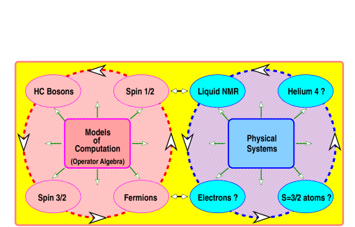
Figure 1: Relationship between different models of computation (with their associated operator algebras) and different physical systems. Question marks refer to the present lack of a quantum computer device using the corresponding elementary physical components indicated in the box. Diamond-shaped arrows represent the natural connection between physical system and operator language, while arrows on the circle indicate the existence of isomorphisms of $*$-algebras, therefore, the corresponding simulation of one physical system by another. A wave function view of this relationship is given in somaroo:qc1999a .

A fundamental concept in quantum information processing is the connection of a quantum computational model to a physical system by transformations of closed operator algebras. The concept is a necessary one because in quantum mechanics each physical system is naturally associated with a language of operators (for example, quantum spin-1/2 operators) and thus to an algebra realizing this language (e.g., the Pauli spin algebra generated by a family of commuting quantum spin-1/2 operators). Any quantum system defined by an algebra of operators generated by a set of “basic” operators can be considered as a possible model of quantum computation sfer . The remarkable fact is that an arbitrary physical system is simulatable by another physical system (or quantum computer) whenever isomorphic mappings (embeddings) between the two operator algebras exists. In each such case, an important problem is to determine whether the simulation is efficient (polynomial resource overhead) in terms of the “basic” generators. For example, a nuclear spin (NMR) quantum computer is modeled as a collection of quantum spin-1/2 objects and described by the Pauli algebra. It can simulate a system of ⁴He atoms (with space discretized by a lattice) represented by the hard-core bosonic algebra, and vice versa. In this case, the simulation is efficient. Figure 1 summarizes this fundamental concept by giving a variety of proposed physical models for quantum computers and associated usable operator algebras. If one of these systems suffices as the universal model of quantum computing, the mappings between the operator algebras establish the equivalence of the other physical models to it. This is one’s intuitive expectation, and has a well-established mathematical basis batista01 .

The mappings between algebras, between an algebra and a physical system, and between physical systems are necessary in order to be able to simulate physical systems using a quantum computer fabricated on the basis of another system. However, this does not imply that the simulation is efficiently implementable. As we have previously discussed sfer , efficient quantum computation involves more than having the ability to represent $2^{N}$ different items of classical information so that the algebra of $N$ quantum bits (qubits) can be isomorphically represented and quantum parallelism can be exploited. It is also insufficient for the mapping between operator algebras to be easily and perhaps efficiently formalized symbolically. For example, the physical system consisting of one boson in $2^{N}$ modes is described using the language of “transition” operators that move the boson from one mode to the other. Formally, the Pauli matrices on $N$ qubits can be easily represented using the transition operators, but the one-boson system is no more powerful than classical wave mechanics. This means that unless quantum computers are not as powerful as is believed, there is no efficient simulation of qubits by the one-boson system.

To be useful as a physics simulation device, a quantum computer must answer questions about physical properties associated with real physical systems. These questions are often concerned with the expectation values of specific measurements of a quantum state evolved from a specific initial state. Consequently, the initialization, evolution, and measurement processes must all be implementable with polynomial scaling sfer . Often it is difficult to do. Further, some classes of measurements, such as thermodynamic ones, still lack well-defined workable algorithms terhal:qc1998a .

On a classical computer, many quantum systems are simulated by the Monte Carlo method qmcrev . For fermions, the operation counts of these Monte Carlo algorithms scale polynomially with the complexity of the system as measured by the number of degrees of freedom, but the statistical error scales exponentially (in time and in number of degrees of freedom), making the simulation ineffective for large systems. A quantum computer allows for the efficient simulation of some systems that are impractical on a classical computer. In our recent paper sfer we discussed how to simulate a system of spinless fermions by the standard model of a quantum computer, that is, the model expressed in the language and algebra of quantum spin-1/2 objects (Pauli algebra). We also discussed how to make certain physically interesting measurements. We demonstrated that the mapping between algebras is a step of polynomial complexity and gave procedures for initial state preparation, evolution, and certain measurements that scaled polynomially with complexity. The main focus of the paper however was demonstrating that a particular problem for simulating fermions on a classical computer, called the dynamical sign problem, does not exist on a quantum computer. We are aware of at least one case where the sign problem can be mapped onto an NP-complete problem wiese . This is the 3-SAT problem farhi01 . Therefore, one cannot yet claim that a quantum computer can solve “all” sign problems, otherwise one would claim that one is solving all NP-complete problems and this has not been rigorously established.

In this paper we continue to explore additional issues associated with efficient and effective simulations of physical systems on a quantum computer, issues which are independent of the particular experimental realization of the quantum computer. We seek to construct quantum network models of such computations. Such networks are sets of elementary quantum gates to which we map our physical system. For simplicity, we discuss these issues relative to simulating a system of spin-1/2 fermions by the standard model of quantum computing. Our discussion has obvious applications to the simulation of a system of bosons (or any other particle statistics or, in mathematical terms, any other operator algebra). Specifically we address issues discovered in our attempt to implement a (classical) simulator of a network-based quantum computer and to conduct a quantum computation on a physical system (NMR) with a small number of qubits. On a classical computer the number of qubits simulatable is limited by the exponential growth of the memory requirements. Physically, we can only process information experimentally with systems of a few qubits. Having the simulator permits a comparison between theory and experiments likely to be realizable in the near future. Overall, the main problems we address are how to reduce the number of qubits and quantum logic gates needed for the simulation of a particular physical phenomena, and how to increase the amount of physical information measurable by designing efficient quantum algorithms.

We organized the paper in the following manner: In Section II we summarize the quantum network representation of the standard model of quantum computation, discussing both one- and multi-qubit circuits. Then we summarize the connection between the spin and fermion representations. In Section III, we first discuss the initialization, evolution, and measurement processes. In each case we define procedures simpler than the ones presented in our previous paper, greatly improving the efficiency with which they can be done. Greatly expanded are the types of measurements now possible. For example, besides certain correlation functions, the spectrum of operators, including the energy operator, can now be obtained. Our application of this technology to a system of fermions on a lattice and the construction of a simulator is discussed in Section IV. The Hubbard model is used as an example. We conclude with a summary and a discussion of areas needing additional work. The appendices contain technical points about the preparation of coherent and correlated states and the use of the discrete classical Fourier transformation.

II Quantum Network Representation of Physical Phenomena

It is the formal connection between models of computation and physical systems described in the Introduction that allows one to simulate quantum phenomena with a quantum computer. Simulation is realized through a quantum algorithm that consists of unitary operations and measurements. One of the objectives is to accomplish simulation efficiently, i.e, with polynomial complexity. The hope is that quantum simulation is “more” efficient (less resources) than classical simulation and there are examples that support such hope sfer . In the following subsections we summarize the main concepts in the representation of physical phenomena by quantum networks.

II.1 Standard Model

In the standard model of quantum computation, the quantum bit, or qubit, is the fundamental unit. A qubit’s state $|{\sf a}\rangle$ is a linear combination of the states $|{0}\rangle$ and $|{1}\rangle$ (e.g, a spin 1/2 with $|{0}\rangle=|{\uparrow}\rangle,\ |{1}\rangle=|{\downarrow}\rangle$):

$$|{\sf a}\rangle=a\ |{0}\rangle+b\ |{1}\rangle\ ,$$ (1)

where the complex numbers $a$ and $b$ are normalized to unity: $|a|^{2}+|b|^{2}=1$.

Assigned to each qubit are the identity matrix ${\mathchoice{\rm 1\mskip-4.0mul}{\rm 1\mskip-4.0mul}{\rm 1\mskip-4.5mul}{\rm 1\mskip-5.0mul}}$ and the Pauli matrices $\sigma_{x}$, $\sigma_{y}$ and $\sigma_{z}$:

$${\mathchoice{\rm 1\mskip-4.0mul}{\rm 1\mskip-4.0mul}{\rm 1\mskip-4.5mul}{\rm 1\mskip-5.0mul}}=\pmatrix{1&0\cr 0&1\cr}\ ,\ \sigma_{x}=\pmatrix{0&1\cr 1&0\cr}\ ,\ \sigma_{y}=\pmatrix{0&-i\cr i&0\cr}\ ,\ \sigma_{z}=\pmatrix{1&0\cr 0&-1\cr}\ ,$$ (2)

or equivalently ${\mathchoice{\rm 1\mskip-4.0mul}{\rm 1\mskip-4.0mul}{\rm 1\mskip-4.5mul}{\rm 1\mskip-5.0mul}}$, $\sigma_{\pm}=\frac{1}{2}(\sigma_{x}{\pm}i\sigma_{y})$, and $\sigma_{z}$. In this particular representation, the states $|{0}\rangle$ and $|{1}\rangle$ are the vectors:

$$|{0}\rangle=\pmatrix{1\cr 0\cr}\mbox{ and }|{1}\rangle=\pmatrix{0\cr 1\cr}\ ,$$ (3)

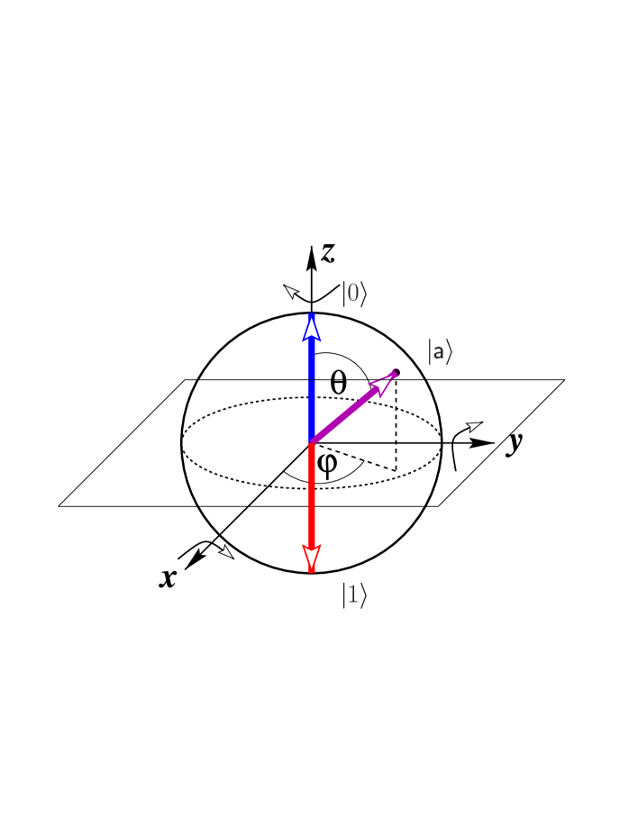
Figure 2: Bloch-Sphere representation of a one qubit state parametrized as $|{\sf a}\rangle=\cos\frac{\theta}{2}|{0}\rangle+e^{i\varphi}\sin\frac{\theta}{2}|{1}\rangle$. The curved arrows indicate the sign of rotation of $e^{i\frac{t}{2}\sigma_{\mu}}=R_{\mu}(-t)$ about the particular axis $\mu$. Our (arrow) color convention is: $|{0}\rangle\rightarrow$ blue; $|{1}\rangle\rightarrow$ red; other linear combinations $\rightarrow$ magenta.

and the Bloch-Sphere (Fig. 2) provides a convenient three-dimensional real space representation of the single qubit state $|{\sf a}\rangle$, which can be parametrized as $|{\sf a}\rangle=\cos\frac{\theta}{2}|{0}\rangle+e^{i\varphi}\sin\frac{\theta}{2}|{1}\rangle$.

For a system of $n$ qubits, the mathematical representation of the standard model is defined by a closed $*$-algebra (Pauli algebra) generated by the operators $\sigma_{\mu}^{j}$ ($\mu=x$, $y$, or $z$) that act on the $j^{th}$ qubit:

$$\sigma^{j}_{\mu}=\overbrace{{\mathchoice{\rm 1\mskip-4.0mul}{\rm 1\mskip-4.0mul}{\rm 1\mskip-4.5mul}{\rm 1\mskip-5.0mul}}\otimes{\mathchoice{\rm 1\mskip-4.0mul}{\rm 1\mskip-4.0mul}{\rm 1\mskip-4.5mul}{\rm 1\mskip-5.0mul}}\otimes\cdots\otimes\underbrace{\sigma_{\mu}}_{j^{th}\ \mbox{factor}}\otimes\cdots\otimes{\mathchoice{\rm 1\mskip-4.0mul}{\rm 1\mskip-4.0mul}{\rm 1\mskip-4.5mul}{\rm 1\mskip-5.0mul}}}^{n\ \mbox{factors}}\ ,$$

where $\otimes$ represents a Kronecker product. From these definitions, the resulting commutation relations are

$${[}\sigma_{\mu}^{j},\sigma_{\nu}^{j}{]}_{+} = 2\delta_{\mu\nu}$$ (4)

$${[}\sigma_{\mu}^{j},\sigma_{\nu}^{k}{]}_{-} = 2i\delta_{jk}\epsilon_{\mu\nu\lambda}\sigma^{j}_{\lambda}\ ,$$ (5)

where $[A,B]_{\pm}=AB{\pm}BA$, and $\epsilon_{\mu\nu\lambda}$ is the totally anti-symmetric Levi-Civita symbol. The time evolution of an $n$ qubit system is described by the unitary operator $\hat{U}(t)=e^{-iHt}$, where $H$ represents the time-independent Hamiltonian of the system. In turn, $\hat{U}(t)$ is easily expressible in terms of the Pauli matrices $\sigma_{\mu}^{j}$ since they and their products form an operator basis of the algebra.

The most general unitary operator ${U}$ on a single qubit can be written as

$${U}=e^{i\alpha}R_{z}(\beta)R_{y}(\gamma)R_{z}(\delta)\ ,$$ (6)

where $\alpha$, $\beta$, $\gamma$, and $\delta$ are real numbers, and $R_{\mu}(\vartheta)=e^{-i\frac{\vartheta}{2}\sigma_{\mu}}$ are rotations in spin space by an angle $\vartheta$ about the $\mu$ axis. Although this decomposition is not unique, it is important because any one qubit evolution is seen to be a combination of simple rotations (up to a phase) about the $\mu=x$, $y$ or $z$ axis.

In multi-qubit operations, any unitary operation ${U}$ can be decomposed (up to a phase) as ${U}=\prod\limits_{l}U_{l}$, where $U_{l}$ are either single qubit rotations $R_{\mu}(\vartheta)$ in the $n$-qubit space or two qubit interactions $R_{z^{j},z^{k}}(\omega)=e^{i{\omega}\sigma_{z}^{j}\sigma_{z}^{k}}$ in the same space ($\omega$ is a real number) barenco:qc1995a ; divincenzo:qc1995a . These one qubit rotations and two qubit interactions constitute the elementary gates of the quantum computer in the network model.

II.2 Quantum Network

We now describe some common one and two qubit gates, some quantum circuits, and one pictorial way to represent them. The motivation for this elementary subsection is to prepare the grounds for the quantum network simulation of a physical system developed in Section III which is more technically involved.

The goal is to represent any unitary operation (evolution) as a product of one and two qubit operations. Although here we use the algebra of the Pauli matrices (standard model), for a different model of computation we should change the set of elementary gates, but the general methodology remains the same. For instance, if the evolution $\hat{U}(t)=e^{-iHt}$ is due to the Hamiltonian

$$H=H_{x}+H_{y}=\bar{\alpha}\ \sigma_{x}^{1}\sigma_{z}^{2}\cdots\sigma_{z}^{j-1}\sigma^{j}_{x}+\bar{\beta}\ \sigma_{y}^{1}\sigma_{z}^{2}\cdots\sigma_{z}^{j-1}\sigma^{j}_{y}\ ,$$ (7)

where $\bar{\alpha}$ and $\bar{\beta}$ are real numbers, we write $\hat{U}(t)$ as $e^{-iH_{x}t}e^{-iH_{y}t}$ because $[H_{x},H_{y}]_{-}=0$. To decompose this into one and two qubit operations, we take the following steps: We first note that the unitary operator

$$U_{1}=e^{i\frac{\pi}{4}\sigma_{y}^{1}}=\frac{1}{\sqrt{2}}\left[{{\mathchoice{\rm 1\mskip-4.0mul}{\rm 1\mskip-4.0mul}{\rm 1\mskip-4.5mul}{\rm 1\mskip-5.0mul}}}+i\sigma_{y}^{1}\right]$$ (8)

takes $\sigma_{z}^{1}\rightarrow\sigma^{1}_{x}$, i.e., $U_{1}^{\dagger}\sigma_{z}^{1}U_{1}=\sigma_{x}^{1}$, so $U_{1}^{\dagger}e^{i{\bar{\alpha}}\sigma_{z}^{1}}U_{1}=e^{i{\bar{\alpha}}\sigma_{x}^{1}}$. Next we note that the operator

$$U_{2}=e^{i{\pi\over 4}\sigma_{z}^{1}\sigma_{z}^{2}}=\frac{1}{\sqrt{2}}\left[{{\mathchoice{\rm 1\mskip-4.0mul}{\rm 1\mskip-4.0mul}{\rm 1\mskip-4.5mul}{\rm 1\mskip-5.0mul}}}+i\sigma_{z}^{1}\sigma_{z}^{2}\right]$$

takes $\sigma^{1}_{x}\rightarrow\sigma^{1}_{y}\sigma^{2}_{z}$, so $U_{2}^{\dagger}e^{i{\bar{\alpha}}\sigma_{x}^{1}}U_{2}=e^{i{\bar{\alpha}}\sigma_{y}^{1}\sigma_{z}^{2}}$. Then we note that

$$U_{3}=e^{i{\pi\over 4}\sigma_{z}^{1}\sigma_{z}^{3}}$$

takes $\sigma^{1}_{y}\sigma^{2}_{z}\rightarrow-\sigma^{1}_{x}\sigma^{2}_{z}\sigma^{3}_{z}$. By successively similar steps we easily build the required string of operators: $\sigma_{x}^{1}\sigma_{z}^{2}\cdots\sigma_{z}^{j-1}\sigma^{j}_{x}$ and also $e^{i{\bar{\alpha}}\sigma_{x}^{1}\sigma_{z}^{2}\cdots\sigma_{z}^{j-1}\sigma^{j}_{x}}$ (up to a global phase):

$$U_{k}^{\dagger}\cdots U_{2}^{\dagger}U_{1}^{\dagger}e^{i{\bar{\alpha}}\sigma_{z}^{1}}U_{1}U_{2}\cdots U_{k}=e^{i{\bar{\alpha}}\sigma_{x}^{1}\sigma_{z}^{2}\cdots\sigma_{z}^{j-1}\sigma^{j}_{x}}\$$ (9)

where the integer $k$ scales polynomially with $j$ (in this particular case the scaling is linear). In a similar way, we decompose the evolution $e^{-iH_{y}t}$. Multiplying both decompositions, we have the total decomposition of the evolution operator $\hat{U}(t)$. See price:qc1999a ; somaroo:qc1998a for complete treatments of these techniques.

II.2.1 Single Qubit Circuits

In Fig. 3a we show examples of several elementary one qubit gates. (Notice that $e^{i\theta\sigma_{\mu}}=R_{\mu}(-2\theta)$.) Each gate applies one or more unitary operations $R_{\mu}(\vartheta)$ to the qubit (the $\sigma_{\mu}$ gates apply a $R_{\mu}(\pi)$ rotation up to a phase: $\sigma_{\mu}=ie^{-i\frac{\pi}{2}\sigma_{\mu}}$). Also, in Fig. 3a we show the Hadamard gate H. The action of this gate on the state of one qubit $|{\sf a}\rangle$ is:

$$\mbox{H}\left\{\begin{array}[]{c}|{0}\rangle\leftrightarrow|{+}\rangle=(|{0}\rangle+|{1}\rangle)/\sqrt{2}\\ |{1}\rangle\leftrightarrow|{-}\rangle=(|{0}\rangle-|{1}\rangle)/\sqrt{2}\end{array}\right.\ .$$

In this way, the Hadamard gate admits the matrix representation:

$$\mbox{H}=\frac{1}{\sqrt{2}}\pmatrix{1&1\cr 1&-1}\ .$$ (10)

In terms of the Pauli matrices

$$\mbox{H}=\frac{1}{\sqrt{2}}[\sigma_{x}+\sigma_{z}]=ie^{-i\frac{\pi}{2}\sigma_{x}}e^{-i\frac{\pi}{4}\sigma_{y}}\ .$$ (11)

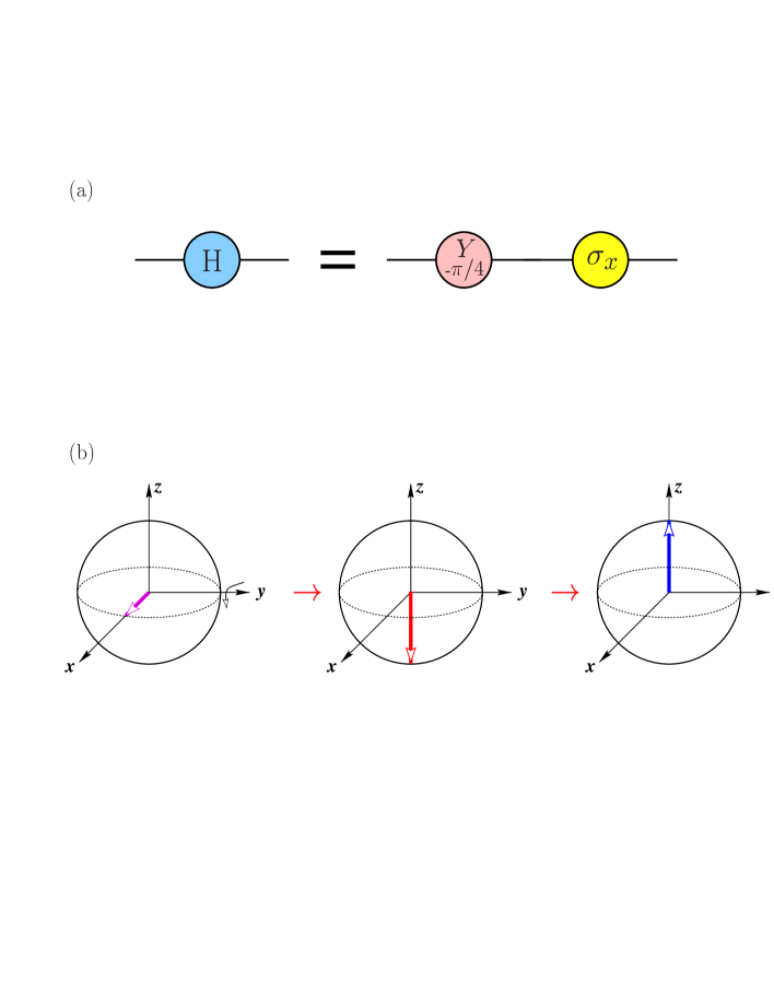
Figure 4: (a) Hadamard gate decomposition and (b) Bloch-Sphere representation of a Hadamard gate applied to the state $|{+}\rangle$.

In Fig. 4a we show the decomposition of the H gate into single qubit rotations, and its application to the Bloch-Sphere representation of the state $|{+}\rangle$ is shown in Fig. 4b. The convention for quantum circuits is each horizontal line represents the time evolution of a single qubit and the time axis of the evolution increases from left to right.

II.2.2 Multiple Qubit Circuits

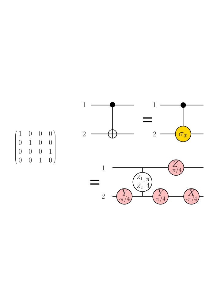
Figure 5: C-NOT gate decomposition and its matrix representation. The control qubit is 1. Note that the last circuit realizes the C-NOT matrix operation up to a global phase $e^{-i\frac{\pi}{4}}$.

We now give examples of multi-qubit operations. Again the goal is to represent them as a combination (up to a phase) of single qubit rotations $R_{\mu}(\vartheta)$ and two qubit interactions $R_{z^{j},z^{k}}(\omega)=e^{i{\omega}\sigma_{z}^{j}\sigma_{z}^{k}}$ (the gate for the $R_{z^{j},z^{k}}(\omega)$ is shown in Fig. 3b). To illustrate this, we consider the circuit shown in Fig. 5. This is a two qubit controlled-NOT (C-NOT) gate which acts as follows:

$$\mbox{C-NOT}\left\{\begin{array}[]{c}|{00}\rangle\rightarrow|{00}\rangle\\ |{01}\rangle\rightarrow|{01}\rangle\\ |{10}\rangle\rightarrow|{11}\rangle\\ |{11}\rangle\rightarrow|{10}\rangle\end{array}\right.\ .$$

Here, the first qubit is the control qubit (the controlled operation on its state $|{1}\rangle$ is represented by a solid circle in Fig. 5). We see that if the state of the first qubit is $|{0}\rangle$ nothing happens, but if the first qubit is in $|{1}\rangle$, then the state of the second qubit is flipped. Because $\sigma_{x}^{2}$ is the unitary operator that flips the second qubit (see Fig. 5), the decomposition of the C-NOT operation into one and two qubits interaction is

$$\mbox{C-NOT: }e^{i\frac{\pi}{4}}e^{-i\frac{\pi}{4}\sigma_{z}^{1}}e^{-i\frac{\pi}{4}\sigma_{x}^{2}}e^{i\frac{\pi}{4}\sigma_{z}^{1}\sigma_{x}^{2}}=e^{i\frac{\pi}{4}}e^{-i\frac{\pi}{4}\sigma_{z}^{1}}e^{-i\frac{\pi}{4}\sigma_{x}^{2}}e^{i\frac{\pi}{4}\sigma_{y}^{2}}e^{-i\frac{\pi}{4}\sigma_{z}^{1}\sigma_{z}^{2}}e^{-i\frac{\pi}{4}\sigma_{y}^{2}}\ .$$ (12)

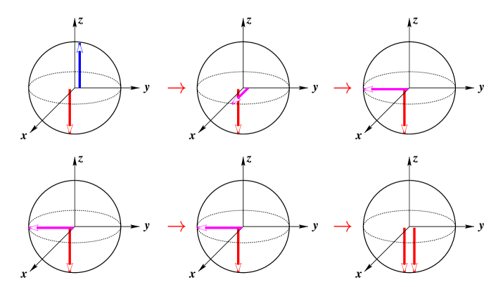
Figure 6: Bloch-Sphere representation of the state obtained by the C-NOT gate applied to the “classical” state $|{10}\rangle$. The sequence of elementary operations is the same as fig. 5 (time flows from left to right with the lower row continuing the upper one). For each Bloch-Sphere the two arrows indicate the states of the two qubits, with the left representing qubit one.

From Eq. 12 we can see that a single controlled operation becomes a greater number (in this case 4) of one and two qubits operations. In Fig. 5 we also show the circuit representing this decomposition, while in Fig. 6 we show the C-NOT gate applied to the state $|{10}\rangle$ in the Bloch-Sphere representation. Because of the control qubit being in the state $|{1}\rangle$, the second qubit is flipped.

A generalization of the C-NOT gate is the controlled-$U$ (C-$U$) gate, where $U$ is a unitary operator acting on a multi-qubit state $|{\Psi_{s}}\rangle$:

$$\mbox{C-$U$}\left\{\begin{array}[]{l}|{0}\rangle_{\sf a}\otimes|{\Psi_{s}}\rangle\rightarrow|{0}\rangle_{\sf a}\otimes|{\Psi_{s}}\rangle\\ |{1}\rangle_{\sf a}\otimes|{\Psi_{s}}\rangle\rightarrow|{1}\rangle_{\sf a}\otimes{\biggl{[}}U|{\Psi_{s}}\rangle{\biggr{]}}\end{array}\right.\ .$$

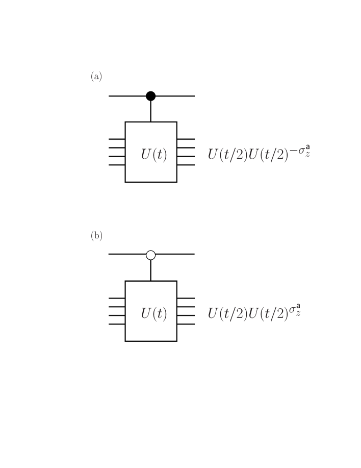
Figure 7: (a) C-$U$ operation with the state of the control qubit ${\sf a}$ being in $|{1}\rangle_{\sf a}$ and (b) C-$U^{\prime}$ operation controlled with the state $|{0}\rangle_{\sf a}$. (See text for notation.)

Mathematically, for $U(t)=e^{-i\hat{Q}t}$ ($\hat{Q}$ is Hermitian), the operational representation of the C-$U$ gate is: $U(t/2)U(t/2)^{-\sigma_{z}^{\sf a}}$ ($U(t)^{-\sigma_{z}^{\sf a}}=e^{i\hat{Q}\otimes{\sigma_{z}^{\sf a}t}}$), where ${\sf a}$ is the control qubit (Fig. 7a). Similarly, one can use $|{0}\rangle_{\sf a}$ as the control state to define the C-$U^{\prime}$ gate illustrated in Fig. 7b. In order to describe the C-$U$ and C-$U^{\prime}$ gates as a combination of single qubit rotations and two qubits interactions, we have to decompose the operators $U(t/2)$ and $U(t/2)^{\sigma_{z}^{\sf a}}$ into such operations. C-$U$ can then be expressed as a sequence of conditional one and two qubit rotations. The latter can be further decomposed into one and two qubit rotations using the techniques of barenco:qc1995a .

II.3 Spin-Fermion connection

To simulate fermionic systems with a quantum computer that uses the Pauli algebra, we first map the fermionic system into the standard model sfer ; bravyi:qc2000a . The commutation relations for (spinless) fermionic operators $a_{j}$ and $a_{j}^{\dagger}$ (the destruction and creation operators for mode $j$) are

$${[}a_{j}^{\dagger},a_{k}{]}_{+} = \delta_{jk}\ ,$$ (13)

$${[}a_{j}^{\dagger},a_{k}^{\dagger}{]}_{+} = 0\ .$$ (14)

We map this set of operators to one expressed in terms of the $\sigma_{\mu}^{j}$’s in the following way:

$$a_{j}^{\;} \rightarrow \left(\prod_{l=1}^{j-1}-\sigma^{l}_{z}\right)\sigma^{j}_{-}=(-1)^{j-1}\ \sigma^{1}_{z}\sigma^{2}_{z}\cdots\sigma^{j-1}_{z}\sigma^{j}_{-}\ ,$$

$$a^{\dagger}_{j} \rightarrow \left(\prod_{l=1}^{j-1}-\sigma^{l}_{z}\right)\sigma^{j}_{+}=(-1)^{j-1}\ \sigma^{1}_{z}\sigma^{2}_{z}\cdots\sigma^{j-1}_{z}\sigma^{j}_{+}\ .$$

Obviously, for the fermionic commutation relations to remain satisfied, the operators $\sigma_{\mu}^{j}$ must satisfy the commutation relations of the Pauli matrices, so a representation for the operators $\sigma_{\mu}^{j}$ are the Pauli matrices.

The mapping just described (indeed it induces an isomorphism of $*$-algebras) is the famous Jordan-Wigner transformation jordan . Using this transformation, we can describe any fermionic unitary evolution in terms of spin operators and therefore simulate fermionic systems by a quantum computer. Although the mapping as given is for spinless fermions and for one-dimensional systems, it extends to higher spatial dimensions and to spin-1/2 fermions by re-mapping each “mode” label into a new label corresponding to “modes” in a one-dimensional chain. In other words, if we want to simulate spin-1/2 fermions in a finite $N_{x}\times N_{y}$ two-dimensional lattice, we map the label of the two-dimensional lattice to an integer number $S$, running from 1 to $2(N_{x}\times N_{y})$. $S$ identifies a mode in the new chain:

$$a_{(j,k);\sigma}^{\;} \rightarrow\tilde{a}_{S}\rightarrow \left(\prod_{l=1}^{S-1}-\sigma^{l}_{z}\right)\sigma^{S}_{-}=(-1)^{S-1}\ \sigma^{1}_{z}\sigma^{2}_{z}\cdots\sigma^{S-1}_{z}\sigma^{S}_{-}\ ,$$

$$a^{\dagger}_{(j,k);\sigma} \rightarrow\tilde{a}_{S}^{\dagger}\rightarrow \left(\prod_{l=1}^{S-1}-\sigma^{l}_{z}\right)\sigma^{S}_{+}=(-1)^{S-1}\ \sigma^{1}_{z}\sigma^{2}_{z}\cdots\sigma^{S-1}_{z}\sigma^{S}_{+}\ ,$$ (15)

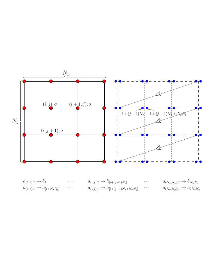
Figure 8: Mapping used to connect the labels of a two-dimensional $N_{x}\times N_{y}$ lattice to the labels of a chain (i.e., a one-dimensional array of integer numbers).

where the $a_{(j,k);\sigma}$ and $a^{\dagger}_{(j,k);\sigma}$ are the fermionic spin-1/2 operators in the two-dimensional lattice for the mode $(j,k)$ and for $z$-component of the spin $\sigma$ ($\sigma=\pm\frac{1}{2}$), and $\tilde{a}_{S}$ and $\tilde{a}_{S}^{\dagger}$ are the spinless fermionic operators in the new chain. In our case, the modes are the sites and the label $(j,k)$ identifies the $X$-$Y$ position of this site ($j,k\in[1,N_{x,y}]$). The label $(j,k);\sigma$ maps into the label $S$ (Fig. 8) via

$$S=j+(k-1)N_{x}+(\frac{1}{2}-\sigma)N_{x}N_{y}\ ,$$ (16)

This is not the only possible mapping to a two-dimensional lattice using Pauli matrices batista01 ; fradkin ; huerta , but it is very convenient for our simulation purposes.

III Quantum Network Simulation of a Physical System

Like the simulation of a physical system on a classical computer, the simulation of a physical system on a quantum computer has three basic steps: the preparation of an initial state, the evolution of the initial state, and the measurement of the physical properties of the evolved state. We will consider each process in turn, but first we note that on a quantum computer there is another important consideration, namely, the relationship of the operator algebra natural to the physical system to the algebra of the quantum network. Fortunately, the mappings (i.e., isomorphisms) between arbitrary representations of Lie algebras are now known batista01 . Section II.3 is just one example. To emphasize this point, the context of our discussion of the three steps will be the simulation of a system of spinless fermions by the standard model, which is representable physically as a system of quantum spin 1/2 objects.

III.1 Preparation of the Initial State

The preparation of the initial state is important because the properties we want to measure (correlation functions, energy spectra, etc.) depend on it. As previously discussed sfer , there is a way to prepare a fermionic initial state of a system with $N_{e}$ spinless fermions and $n$ single particle modes $j$, created by the operators $a_{j}^{\dagger}$ ( creation of a fermion in the mode $j$). In the most general case, the initial state is a linear combination of Slater determinants

$$|{\Phi_{\alpha}}\rangle=\prod\limits_{j=1}^{Ne}b_{j}^{\dagger}\ |{\rm vac}\rangle\ ,$$ (17)

described by the fermionic operators $b_{j}$ and $b_{j}^{\dagger}$, which are related to the operators $a_{j}$ and $a_{j}^{\dagger}$ via a canonical (unitary) transformation. Here $|{\rm vac}\rangle$ is the vacuum state (zero particle state). To prepare $|{\Phi_{\alpha}}\rangle$ one can look for unitary transformations $U_{m}$ such that

$$|{\Phi_{\alpha}}\rangle=e^{i\gamma}\prod\limits_{m=1}^{Ne}U_{m}\ |{\rm vac}\rangle\ ,$$ (18)

where $\gamma$ is a phase factor. To perform these operations in the standard model we must express the $U_{m}$ in terms of Pauli matrices using the Jordan-Wigner transformation. (We can do the mapping between the Pauli operators and the $a_{j}$ operators or between the Pauli operators and the $b_{j}$ operators. In the following we will assume the first mapping since this will simplify the evolution step.) One can choose $U_{m}=e^{-iH_{m}t}$ such that $H_{m}$ is linear in the $b_{m}$ and $b_{m}^{\dagger}$ operators sfer . We have to decompose the $U_{m}$ into single qubit rotations and two qubit interactions $R_{\mu}(\vartheta)\mbox{ and }R_{z^{j},z^{k}}(\omega)$. To do this, we first decompose the $U_{m}$ into a products of operators linear in the $b_{m}$ or $b_{m}^{\dagger}$; however, this decomposition does not conserve the number of particles. The situation appears complex.

Simplification occurs, however, by recalling the Thouless’s theorem blaizot which says that if

$$|{\phi}\rangle=\prod\limits_{j=1}^{N_{e}}a^{\dagger}_{j}\ |{\rm vac}\rangle$$ (19)

and $M$ is a $n\times n$ Hermitian matrix, then

$$e^{i\vec{a}^{\dagger}M\vec{a}}\ |{\phi}\rangle=\prod\limits_{j=1}^{N_{e}}b^{\dagger}_{j}\ |{\rm vac}\rangle\ ,$$ (20)

where $\vec{a}^{\dagger}=(a^{\dagger}_{1},\cdots,a^{\dagger}_{n})$ and

$$\vec{b}^{\dagger}=e^{iM}\ \vec{a}^{\dagger}\ .$$ (21)

From Eq. 21 the operator $e^{iM}$ (formally acting on the vector of $a^{\dagger}_{j}$’s) realizes the canonical transformation between $a_{j}$ and $b_{j}$.

Thouless’s theorem generalizes to quantum spin systems via the Jordan-Wigner transformation. This theorem allows the preparation of an initial state by simply applying the unitary operator $e^{i\vec{a}^{\dagger}M\vec{a}}$ to a “boot up” state polarized with each qubit being in the state $|{0}\rangle$ or $|{1}\rangle$. Indeed, for an arbitrary Lie operator algebra the general states prepared in this fashion are known as Perelomov-Gilmore coherent states peregilmo .

The advantage of this theorem for preparing the initial state instead of the method previously described sfer is that the decomposition of the unitary operator $e^{i\vec{a}^{\dagger}M\vec{a}}$ can be done in steps, each using combinations of operators $a_{j}a_{k}^{\dagger}$ and, therefore, conserving the number of particles. Once the decomposition is done, we then write each operator in terms of the Pauli operators to build a quantum circuit in the standard model. (See Appendix A for a simple example.)

A single Stater determinant is a state of independent particles. That is, from the particle perspective, it is unentangled. Generically, solutions to interacting many-body problems are entangled (correlated) states, that is, a linear combination of many Slater determinants not expressible as a single Slater determinant. In particular, this is the case if the interactions are strong at short ranges. In quantum many-body physics, considerable experience and interest exists in developing simple approaches for generating several specific classes of correlated wave functions blaizot . In Appendix A we illustrate procedures and recipes to prepare one such class of correlated (entangled) states, the so-called Jastrow states blaizot .

III.2 Evolution of Initial State

The evolution of a quantum state is the second step in the realization of a quantum circuit. The goal is to decompose this evolution into the “elementary gates” $R_{\mu}(\vartheta)\mbox{ and }R_{z^{j},z^{k}}(\omega)$. To do this for a time-independent Hamiltonian, we can write the evolution operator as $\hat{U}(t)=e^{-iHt}$, where $H=\sum\limits_{l}H_{l}$ is a sum of individual Hamiltonians $H_{l}$. If the commutation relations ${[}H_{l},H_{l^{\prime}}{]}_{-}=0$ hold for all $l$ and $l^{\prime}$, then

$$\hat{U}(t)=\prod\limits_{l}U_{l}(t)=\prod\limits_{l}e^{-iH_{l}t}\ .$$ (22)

In this way, we can then decompose each $U_{l}(t)$ in terms of one and two qubits interactions, using the method described in Section II.2.

In general, the Hamiltonians $H_{l}$ for different $l$ do not commute and the relation Eq. 22 cannot be used. Although we can in principle exactly decompose the operator $\hat{U}(t)$ into one and two qubit interactions barenco:qc1995a ; divincenzo:qc1995a , such a decomposition is usually very difficult. To avoid this problem, we decompose the evolution $\hat{U}(t)=\prod\limits_{j}^{\cal M}e^{-iH\Delta t}$ using the the first-order Trotter approximation ($t={\cal M}\Delta t$):

$$\hat{U}(\Delta t)=e^{-iH\Delta t}=e^{-i\sum\limits_{l}H_{l}\Delta t}=\prod_{l}e^{-iH_{l}\Delta t}+{\cal O}((\Delta t)^{2})\ .$$ (23)

Then, for $\Delta t\rightarrow 0$, we can approximate the short-time evolution by: $\hat{U}(\Delta t)\approx\prod\limits_{l}e^{-iH_{l}\Delta t}$. In general, each factor is easily written as one and two qubit operations (Section II.2).

The disadvantage of this method is that approximating the operator $\hat{U}(t)$ with high accuracy might require $\Delta t$ to be very small so the number of steps $e^{-iH_{l}\Delta t}$ and hence the number of quantum gates required becomes very large. To mitigate this problem, we can use a higher-order Trotter decomposition. For example, if $H=K+V$, we then use the second-order Trotter approximation to decompose the evolution as $\hat{U}(t)=\prod\limits_{j}e^{-iH\Delta t}$ with (second-order decomposition)

$$e^{-iH\Delta t} = e^{-iK\frac{\Delta t}{2}}e^{-iV\Delta t}e^{-iK\frac{\Delta t}{2}}+{\cal O}((\Delta t)^{3})\ ,$$ (24)

$$= e^{-iV\frac{\Delta t}{2}}e^{-iK\Delta t}e^{-iV\frac{\Delta t}{2}}+{\cal O}((\Delta t)^{3})\ .$$ (25)

Other higher-order decompositions are available suzuki .

III.3 Measurement of Physical Quantities

III.3.1 One-Ancilla Qubit Measurement Processes

The last step is the measurement of the physical properties of the system that we want to study. Often we are interested in measurements of the form $\langle U^{\dagger}V\rangle$, where $U$ and $V$ are unitary operators sfer . We refer to Ref. sfer for a description of the type of correlation functions that are related to these measurements. See also paz for an application and variation of these techniques. Here, we simply give a brief description of how to perform such measurements.

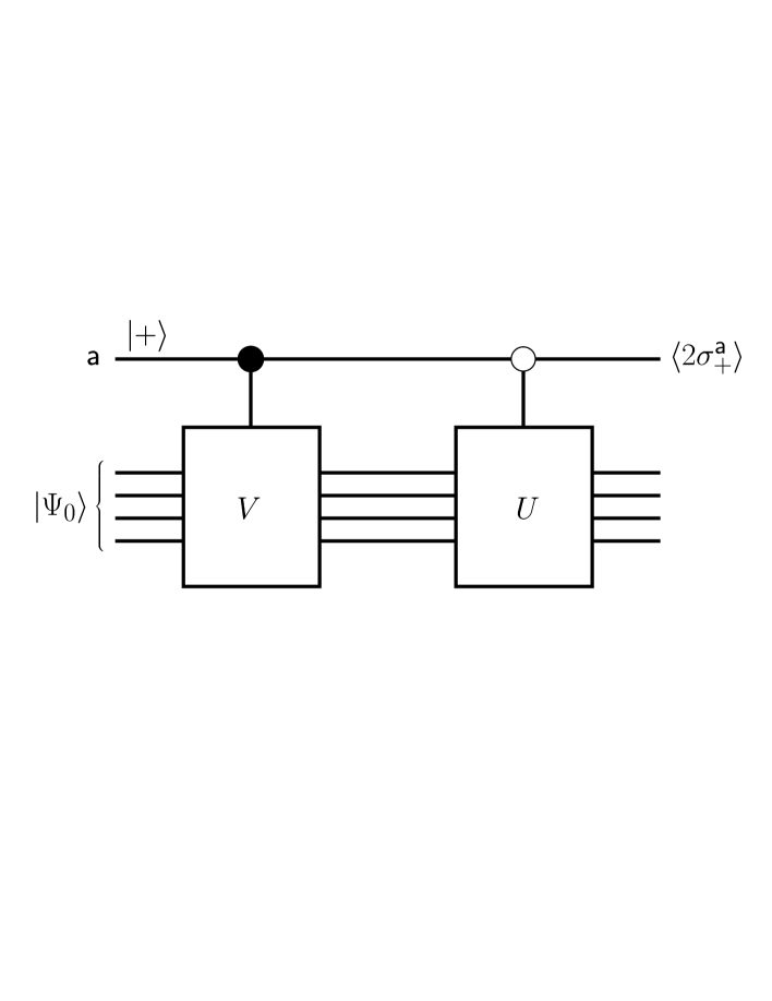
Figure 9: Measurement of physical quantities using one extra (ancilla) qubit $|{\sf a}\rangle$. In this case $\langle 2\sigma^{\sf a}_{+}\rangle=\langle\Psi_{0}|U^{\dagger}V|{\Psi_{0}}\rangle$.

First, we prepare the system in the initial state $|{\Psi_{0}}\rangle$ and adjoin to it one ancilla (auxiliary) qubit $\sf a$, in the state $|{+}\rangle=(|{0}\rangle+|{1}\rangle)/\sqrt{2}$. This is done by applying the unitary Hadamard gate to the state $|{0}\rangle$ (Fig. 4). Next, we make two controlled unitary evolutions using the C-$U$ and C-$U^{\prime}$ gates. The first operation $\tilde{V}$ evolves the system by $V$ if the ancilla is in the state $|{1}\rangle$: $\tilde{V}=|{0}\rangle\langle{0}|\otimes{\mathchoice{\rm 1\mskip-4.0mul}{\rm 1\mskip-4.0mul}{\rm 1\mskip-4.5mul}{\rm 1\mskip-5.0mul}}+|{1}\rangle\langle{1}|\otimes V$. The second one $\tilde{U}$ evolves the system by $U$ if the ancilla state is $|{0}\rangle$: $\tilde{U}=|{0}\rangle\langle{0}|\otimes U+|{1}\rangle\langle{1}|\otimes{\mathchoice{\rm 1\mskip-4.0mul}{\rm 1\mskip-4.0mul}{\rm 1\mskip-4.5mul}{\rm 1\mskip-5.0mul}}$. ($\tilde{V}$ and $\tilde{U}$ commute.) Once these evolutions are done, the expectation value of $2\sigma^{\sf a}_{+}=\sigma^{\sf a}_{x}+i\sigma^{\sf a}_{y}$ gives the desired result. This quantum circuit is shown in Fig. 9. Note that the probabilistic nature of quantum measurements implies that the desired expectation value is obtained with variance ${\cal O}(1)$ for each instance. Repetition can be used to reduce the variance below what is required.

III.3.2 $L$-Ancilla Qubit Measurement Processes

Often, we want to compute the expectation value of an operator O of the form

$$O=\sum\limits_{i=1}^{M}a_{i}\ U^{\dagger}_{i}V_{i}\ ,$$ (26)

where $U_{i}$ and $V_{i}$ are unitary operators, $a_{i}$ are real positive numbers ($a_{i}\geq 0$), and $M$ is an integer power of 2. (In the case that $M$ is less than a power of two, we can complete this definition by setting the $a_{M+1},\cdots,a_{M^{\prime}}=0$, where $M^{\prime}$ is an integer power of two.) We can compute this expectation value by preparing $M$ different circuits, each one with one ancilla qubit, and for each circuit measure $\langle U^{\dagger}_{i}V_{i}\rangle$ (see Section III.3.1). Then, we multiply each result by the constant $a_{i}$ and sum the results. However, in most cases, the preparation of the initial state is very difficult. There is another way to measure this quantity by using only one circuit which reduces the difficulty.

We first write the operator O as

$$O={\cal N}\sum\limits_{i=1}^{M}\alpha_{i}^{2}\ U^{\dagger}_{i}V_{i}\ ,$$ (27)

where ${\cal N}=\sum\limits_{i=1}^{M}a_{i}$ and $\alpha_{i}^{2}=a_{i}/{\cal N}$ ($\sum\limits_{i=1}^{M}\alpha_{i}^{2}=1$). Then we construct a quantum circuit with the following steps:

• Prepare the state $|{\Psi_{0}}\rangle$ such that $\langle\Psi_{0}|O\Psi_{0}\rangle$ is the expectation value to be computed.

• Adjoin $L$ ancillas to the initial state, where $L=J+1$ and $2^{J}=M$. The first of these ancillas, ${\sf a}_{1}$, is prepared in the state $|{+}\rangle=(|{0}\rangle+|{1}\rangle)/\sqrt{2}$. This is done by applying the Hadamard gate to the initial state $|{0}\rangle$ (see Fig. 4a). The other ancillas, $\{{\sf a}_{2},{\sf a}_{3},\cdots,{\sf a}_{L}\}$ are kept in the state $|{0}\rangle$.

• Apply a unitary evolution $E(\alpha_{1},\alpha_{2},\cdots,\alpha_{M})$ to the ancillas $\{{\sf a}_{2},{\sf a}_{3},\cdots,{\sf a}_{L}\}$ to obtain

  $$|{\psi}\rangle=\alpha_{1}|{00\cdots 0}\rangle+\alpha_{2}|{00\cdots 1}\rangle+\cdots+\alpha_{M}|{11\cdots 1}\rangle=\sum\limits_{i=1}^{M}\alpha_{i}\ |{i}\rangle\ ,$$

  where $|{i}\rangle$ is a tensorial product of the states ($|{0}\rangle\mbox{ or }|{1}\rangle$) of each ancilla: $|{i}\rangle=|{\eta}\rangle_{{\sf a}_{2}}\otimes\cdots\otimes|{\eta}\rangle_{{\sf a}_{L}}$, where $\eta$ can be 0 or 1. The index $i$ orders the orthonormal basis $|{i}\rangle$.

• Apply the controlled unitary operations $\tilde{U}_{i}$ which evolve the system by $U_{i}$ if the state of the ancillas is $|{0}\rangle_{{\sf a}_{1}}|{i}\rangle$. Then apply the controlled unitary operations $\tilde{V}_{i}$ which evolve the system by $V_{i}$ if the state of the ancillas is $|{1}\rangle_{{\sf a}_{1}}|{i}\rangle$. Once these evolution steps are finished, the state of the whole system is

  $$|{\Psi}\rangle=\frac{1}{\sqrt{2}}\Biggl{[}|{0}\rangle_{{\sf a}_{1}}\sum\limits_{i=1}^{M}\alpha_{i}\ |{i}\rangle\ U_{i}+|{1}\rangle_{{\sf a}_{1}}\sum\limits_{i=1}^{M}\alpha_{i}\ |{i}\rangle\ V_{i}\Biggr{]}\otimes|{\Psi_{0}}\rangle\ .$$

• Measure the expectation value of $2\sigma^{{\sf a}_{1}}_{+}=\sigma^{{\sf a}_{1}}_{x}+i\sigma^{{\sf a}_{1}}_{y}=2|{0}\rangle_{{\sf a}_{1}}\langle{1}|$. It is easy to see that it corresponds to the expectation value of the operator $\sum\limits_{i=1}^{M}\alpha_{i}^{2}\ U^{\dagger}_{i}V_{i}$.

• Obtain the expectation value of O by multiplying $\langle 2\sigma^{{\sf a}_{1}}_{+}\rangle$ by the constant ${\cal N}$.

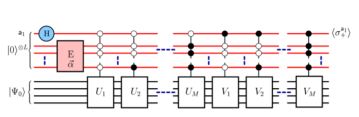
Figure 10: Measurement of physical quantities using $L$-ancillas qubits $\{{\sf a}_{1},\cdots,{\sf a}_{L}\}$. In this case $\langle\sigma^{\sf a_{1}}_{+}\rangle=\frac{1}{2{\cal N}}\langle\Psi_{0}|{[}\sum\limits_{i=1}^{M}a_{i}U^{\dagger}_{i}V_{i}{]}|\Psi_{0}\rangle$ (see text).

The quantum circuit for this procedure is given in Fig. 10.

III.3.3 Measurement of Correlation Functions

We now consider measuring correlation functions of the form $C_{AB}=\langle T^{\dagger}ATB\rangle$, where $T$ is a unitary operator and $A$ and $B$ are operators that are expressible as a sum of unitary operators:

$$A=\sum\limits_{i}\alpha_{i}A_{i}\mbox{ and }B=\sum\limits_{j}\beta_{j}B_{j}.$$ (28)

The operator $T$ is fixed by the type of correlation function that we want to evaluate. In the case of dynamical correlation functions, $T$ is $e^{-iHt}$ where $H$ is the Hamiltonian of the system. For spatial correlation functions, $T$ is the space translation operator $e^{-ip\cdot x}$ ($p$ and $x$ are configuration space operators). The method for measuring these correlation functions is the same method described in Section  III.3.1 or Section  III.3.2. We can use either the one- or the $L$-ancillas measurement process.

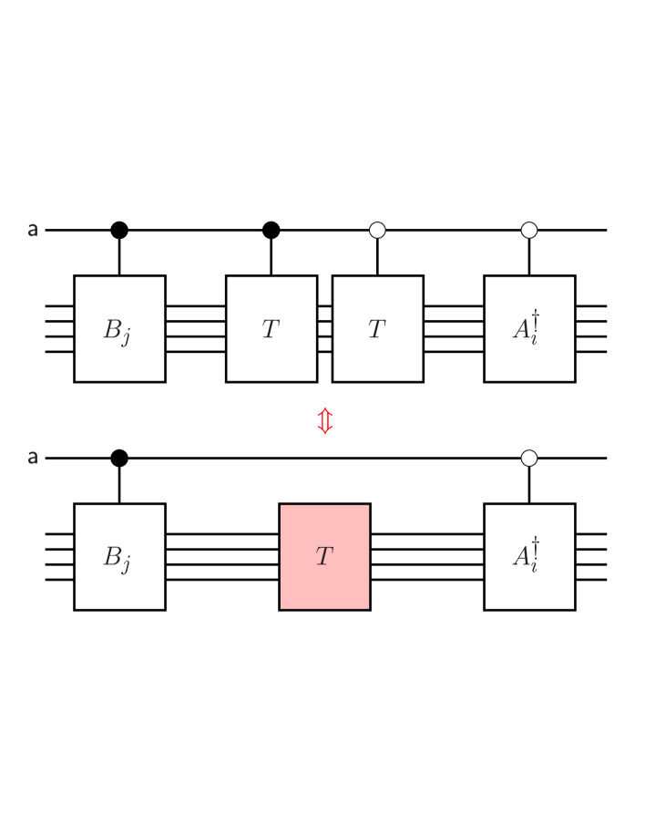
Figure 11: Circuit for the measurement of spatial and time correlation functions. In this case $\langle 2\sigma_{+}^{\sf a}\rangle=\langle T^{\dagger}A_{i}TB_{j}\rangle$. Notice the simplification achieved by reducing two C-$T$ operations into only one uncontrolled $T$ operation.

To minimize the number of controlled operations and also the quantity of elementary gates involved, we choose $U^{\dagger}_{i}=T^{\dagger}A_{i}$ and $V_{j}=TB_{j}$. Now, we have to compute $\langle U^{\dagger}_{i}V_{j}\rangle$. In Fig. 11 we show the circuit for measuring this quantity, where the circuit has only one ancilla in the state $|{+}\rangle=(|{0}\rangle+|{1}\rangle)/\sqrt{2}$. There, the controlled operations were reduced by noting that the operation of $T$ controlled on the state $|{0}\rangle$ of the ancilla followed by the operation of $T$ controlled on the state $|{1}\rangle$, results in a no-controlled $T$ operation. This is a very useful algorithmic simplification.

III.3.4 Measurement of the Spectrum of an Hermitian Operator

Many times one is interested in determining the spectrum of an observable (Hermitian operator) $\hat{Q}$, a particular case being the Hamiltonian $H$. Techniques for getting spectral information can be based on the quantum Fourier transform kitaev ; cleve and can be applied to physical problems abrams . For our purposes, the methods of the previous Sections yield much simpler measurements without loss of spectral information. For a given $H$, the most common type of measurement is the computation of its eigenvalues or at least its lowest eigenvalue (the ground state energy). To do this we start from an state $|{\phi}\rangle$ that has a non-zero overlap with the eigenstates of $H$. (For example, if we want to compute the energy of the ground state, then $|{\phi}\rangle$ has to have a non-zero overlap with the ground state.) For finite systems, $|{\phi}\rangle$ can be the solution of a mean-field theory (a Slater determinant in the case of fermions or Perelomov-Gilmore coherent states in the general case). Once we prepare this state (Section  III.1 and Appendix A), we compute $\langle\hat{U}(t)\rangle=\langle\phi|\hat{U}(t)\phi\rangle$, where $\hat{U}$ is the evolution operator $\hat{U}(t)=e^{-iHt}$. We then note that

$$|{\phi}\rangle=\sum\limits_{n=0}^{\cal L}\gamma_{n}\ |{\Psi_{n}}\rangle\ ,$$ (29)

with $|{\Psi_{n}}\rangle$ eigenstates of the Hamiltonian $H$. Consequently

$$\langle\hat{U}(t)\rangle=\sum\limits_{n=0}^{\cal L}|\gamma_{n}|^{2}\ e^{-i{\lambda}_{n}t}\ ,$$ (30)

where ${\lambda}_{n}$ are the eigenvalues of $H$. The measurement of $\langle\hat{U}(t)\rangle$ is easily done by the steps described in Section III.3.1 (setting $V=\hat{U}(t)$ and $U={\mathchoice{\rm 1\mskip-4.0mul}{\rm 1\mskip-4.0mul}{\rm 1\mskip-4.5mul}{\rm 1\mskip-5.0mul}}$ in Fig. 9). Once we have this expectation value, we perform a classical fast Fourier transform (i.e., $\int\langle\hat{U}(t)\rangle e^{i\lambda t}dt$) and obtain the eigenvalues $\lambda_{n}$ (see Appendix B):

$$\mbox{FFT}[\langle\hat{U}(t)\rangle]=\sum\limits_{n=0}^{\cal L}2\pi|\gamma_{n}|^{2}{\delta}({\lambda}-{\lambda}_{n})\ .$$ (31)

Although we explained the method for the eigenvalues of $H$, the extension to any observable $\hat{Q}$ is straightforward, taking $\hat{U}(t)=e^{-i\hat{Q}t}$ and proceeding in the same way.

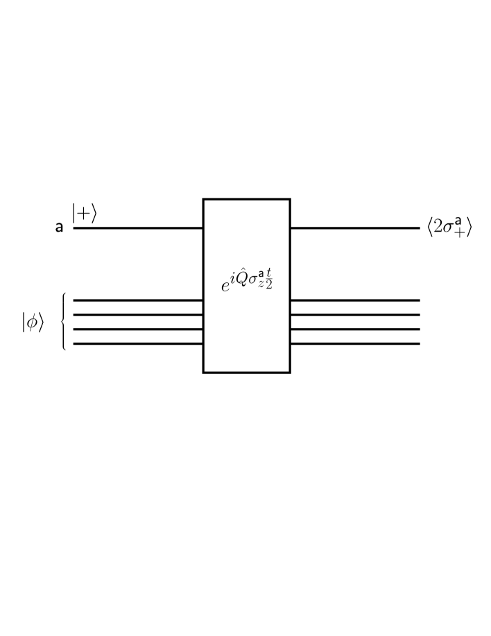
Figure 12: Circuit for the measurement of the spectrum of an Hermitian operator $\hat{Q}$. In this case $\langle 2\sigma^{\sf a}_{+}\rangle=\langle\phi|e^{-i\hat{Q}t}\phi\rangle$ (see text).

Two comments are in order. The first refers to an algorithmic optimization and points to decreasing the number of controlled operations (i.e., the number of elementary gates implemented). If we set $V=e^{-i\hat{Q}t}$, $U^{\dagger}={\mathchoice{\rm 1\mskip-4.0mul}{\rm 1\mskip-4.0mul}{\rm 1\mskip-4.5mul}{\rm 1\mskip-5.0mul}}$ (see Fig. 9) and perform the type of measurement described in Section III.3.1 the network has total evolution (ancilla plus system) $e^{-i\hat{Q}\frac{t}{2}}e^{i\hat{Q}\sigma_{z}^{\sf a}\frac{t}{2}}$, while if we set $V=U^{\dagger}=e^{-i\hat{Q}\frac{t}{2}}$ the total evolution is $e^{i\hat{Q}\sigma_{z}^{\sf a}\frac{t}{2}}$. Thus, this last algorithm reduces the number of gates by the number of gates it takes to represent the operator $e^{-i\hat{Q}\frac{t}{2}}$. The circuit is shown in Fig. 12.

The second comment refers to the complexity of the quantum algorithm as measured by system size. In general it is difficult to find a state whose overlap scales polynomially with system size. If one chooses a mean-field solution as the initial state, then the overlap decreases exponentially with the system size; this is a “signal problem” which also arises in probabilistic classical simulations of quantum systems. The argument goes as follows: If $|\phi\rangle$ is a mean-field state for an $N^{d}$(=volume) system size whose (modulus of the) overlap with the true eigenstate is $|\gamma|<1$, and assuming that the typical correlation length of the problem $\xi$ is smaller than the linear dimension $N$, if we double $N$ the new overlap is $\sim e^{2^{d}\ln|\gamma|}$.

We would like to mention that an alternative way of computing part of the spectrum of an Hermitian operator is using the adiabatic connection or Gell-Mann-Low theorem, an approach that has been described in sfer .

III.3.5 Mixed and Exact Estimators

We already explained how to compute different types of correlation functions. But in most cases, we do not know the state whose correlations we want to obtain. The most common case is wanting the correlations in the ground state $|{\Psi_{0}}\rangle$ of some Hamiltonian $H$. Obtaining the ground state is a very difficult task; however, there are some useful methods to approximate these correlation functions.

Suppose we are interested in the mean value of a unitary operator $O(t)$. If we can prepare the initial state $|{\Psi_{T}}\rangle$ in such a way that $|{\Psi_{0}}\rangle=|{\Psi_{T}}\rangle+\epsilon|{\Phi}\rangle$ ($\epsilon$ is intended to be small), then after some algebraic manipulations negele:qc1988a , we have

$$\frac{\langle{\Psi_{0}}|O(t)|{\Psi_{T}}\rangle}{\langle\Psi_{0}|\Psi_{T}\rangle}=\frac{1}{2}\left[\frac{\langle{\Psi_{0}}|O(t)|{\Psi_{0}}\rangle}{\langle\Psi_{0}|\Psi_{0}\rangle}+\frac{\langle{\Psi_{T}}|O(t)|{\Psi_{T}}\rangle}{\langle\Psi_{T}|\Psi_{T}\rangle}\right]+{\cal O}(\epsilon^{2})$$ (32)

where the term on the left-hand side of Eq. 32 is known as the “mixed estimator.” Also, we can calculate the second term on the right-hand side of Eq. 32 with an efficient quantum algorithm, since we are able to prepare easily $|{\Psi_{T}}\rangle$. Next, we show how to determine the mixed estimator using a quantum algorithm.

If $|{\Psi_{0}}\rangle$ is the ground state, then it is an eigenstate of the evolution operator $\hat{U}(t^{\prime})=e^{-iHt^{\prime}}$, and we can obtain the mixed estimator by measuring the mean value of $\hat{U}(t^{\prime})O(t)$: Because $|{\Psi_{T}}\rangle=\sum\limits_{n}a_{n}|{\Psi_{n}}\rangle$ where $a_{n}=\langle\Psi_{n}|\Psi_{T}\rangle$ and $|{\Psi_{n}}\rangle$ are the eigenstates of $H$ ($\hat{U}(t^{\prime})|{\Psi_{n}}\rangle=e^{-i\lambda_{n}t^{\prime}}|{\Psi_{n}}\rangle$) we can measure (Section  III.3.3)

$$\langle{\Psi_{T}}|\hat{U}(t^{\prime})O(t)|{\Psi_{T}}\rangle=\sum\limits_{n}e^{i\lambda_{n}t^{\prime}}\langle\Psi_{T}|\Psi_{n}\rangle\langle{\Psi_{n}}|O(t)|{\Psi_{T}}\rangle$$ (33)

By performing a Fourier transform in the variable $t^{\prime}$ ($\tilde{F}(\omega)=\int e^{i\omega t^{\prime}}F(t^{\prime})dt^{\prime}$) in Eq. 33 and making the relation between the expectation value for time $t$ and the expectation value for $O(t)={\mathchoice{\rm 1\mskip-4.0mul}{\rm 1\mskip-4.0mul}{\rm 1\mskip-4.5mul}{\rm 1\mskip-5.0mul}}$, we obtain the value of the mixed estimator. Then, by using Eq. 32, we obtain $\frac{\langle{\Psi_{0}}|O(t)|{\Psi_{0}}\rangle}{\langle\Psi_{0}|\Psi_{0}\rangle}$ up to order $\epsilon^{2}$.

By similar steps, we can obtain expectation values of the form $\frac{\langle{\Psi_{n}}|O(t)|{\Psi_{n^{\prime}}}\rangle}{\langle\Psi_{n}|\Psi_{n^{\prime}}\rangle}$ for all $n$ and $n^{\prime}$. The trick consists of measuring (Section  III.3.3) the mean value of the operator $\hat{U}(t^{\prime})O(t)\hat{U}^{\dagger}(t^{\prime\prime})$ in the state $|{\Psi_{T}}\rangle$

$$\langle{\Psi_{T}}|\hat{U}(t^{\prime})O(t)\hat{U}^{\dagger}(t^{\prime\prime})|{\Psi_{T}}\rangle=\sum\limits_{n,n^{\prime}}e^{i\lambda_{n}t^{\prime}}e^{i\lambda_{n^{\prime}}t^{\prime\prime}}\langle\Psi_{T}|\Psi_{n}\rangle\langle\Psi_{n^{\prime}}|\Psi_{T}\rangle\langle{\Psi_{n}}|O(t)|{\Psi_{n^{\prime}}}\rangle$$ (34)

and then by performing a double Fourier transform in the variables $t^{\prime}$ and $t^{\prime\prime}$ ($\tilde{F}(\lambda,\lambda^{\prime})=\int e^{i\lambda t^{\prime}}e^{i\lambda^{\prime}t^{\prime\prime}}F(t^{\prime},t^{\prime\prime})dt^{\prime}dt^{\prime\prime}$) we obtain the desired results. A particular case of this procedure is the direct computation of the exact estimator $\frac{\langle{\Psi_{n}}|O(t)|{\Psi_{n}}\rangle}{\langle\Psi_{n}|\Psi_{n}\rangle}$.

IV Application to Fermionic Lattice Systems

In this Section, we illustrate a procedure for simulating fermionic systems on a quantum computer, showing as a particular example how to obtain the energy spectrum of the Hubbard Hamiltonian for a finite-sized system. We will obtain this spectrum through a simulation of a quantum computer on a classical computer, that is, by a quantum simulator.

We start by noting that the spin-fermion connection described in Eq. II.3 and Eq. 16 implies that the number of qubits involved in a two-dimensional lattice is $L=2(N_{x}\times N_{y})$ if one uses the standard model to simulate spin-1/2 fermions. Also, the number of states for an $L$-qubits system is $2^{L}$. From this mapping, the first $N_{x}\times N_{y}$ qubits represent the states which have spin-up fermions, and the other qubits ($(N_{x}\times N_{y}+1)$ to $2(N_{x}\times N_{y})$) spin-down fermions. In other words, if we have a system of 4 sites and have a state $|{\Psi}\rangle$ with one electron with spin up at the first site and one electron with spin down at the third site, then this state in second quantization is $|{\Psi}\rangle=a_{1;\uparrow}^{\dagger}a_{3;\downarrow}^{\dagger}|{\mbox{vac}}\rangle$, where the fermionic operator $a_{j;\sigma}^{\dagger}$ creates a fermion in the site $j$ with spin $\sigma$, and $|{\mbox{vac}}\rangle$ is the state with no particles (vacuum state). In the standard model, this state corresponds to

$$|{\Psi}\rangle=\sigma_{+}^{1}\prod_{l=1}^{6}\sigma_{z}^{l}\sigma_{+}^{7}|{\widetilde{\mbox{vac}}}\rangle=|{0}\rangle\otimes|{1}\rangle\otimes|{1}\rangle\otimes|{1}\rangle\otimes|{1}\rangle\otimes|{1}\rangle\otimes|{0}\rangle\otimes|{1}\rangle\rightarrow|{\uparrow\downarrow\downarrow\downarrow\downarrow\downarrow\uparrow\downarrow}\rangle,$$ (35)

where $|{\widetilde{\mbox{vac}}}\rangle$ is the vacuum of the quantum spin 1/2, which we have chosen to be $|{\downarrow\downarrow\downarrow\downarrow\downarrow\downarrow\downarrow\downarrow}\rangle$.

To represent the $L$-qubit system on a classical computer, we can build a one-to-one mapping between the $2^{L}$ possible states and the bit representation of an integer $I$ defined by

$$I=\sum\limits_{i=1}^{L}[n(i)\times 2^{i-1}]$$ (36)

where $n(i)$ (occupancy) is 0 if the spin of the $i$-qubit is $|{1}\rangle$ ($\downarrow$), or 1 if the state is $|{0}\rangle$ ($\uparrow$). In this way, the state described in Eq. 35 maps to $I=65$. Because we are interested in obtaining some of the eigenvalues of the Hubbard model, we added an ancilla qubit (Fig. 12). The “new” system has $L=2(N_{x}\times N_{y})+1$ qubits, and we can perform the mapping in the same way described above.

To simulate the evolution operator $\hat{U}(t)=e^{-iHt}$ on a classical computer using the above representation of quantum states, we programmed the “elementary” quantum gates of one and two qubits interactions. Each $L$-qubit state was represented by a linear combination of the integers $I$ (Eq. 36). In this way, each unitary operation applied to one or two qubits modifies $I$ by changing a bit. For example, if we flip the spin of the first qubit, the number $I$ changes by 1.

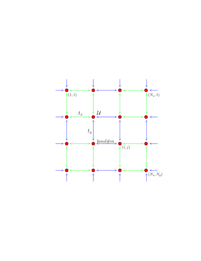
Figure 13: Two-dimensional lattice in the Hubbard model. Here, the green and blue arrows identify the even and odd bonds.

We want to evaluate some eigenvalues of the spin-1/2 Hubbard model in two spatial dimensions. The model is defined on a rectangle of $N_{x}\times N_{y}$ sites and is parametrized by spin preserving hoppings $t_{x}$ and $t_{y}$ between nearest neighbor sites, and an interaction $\cal U$ on site between fermions of different $z$-component of spin (Fig. 13). The Hamiltonian is

$$H=-\sum\limits_{(i,j);\sigma}[ \!\!\!\!\!\!t_{x}(a^{\dagger}_{(i,j);\sigma}a_{(i+1,j);\sigma}^{\;}+a^{\dagger}_{(i+1,j);\sigma}a_{(i,j);\sigma})^{\;}+t_{y}(a^{\dagger}_{(i,j);\sigma}a_{(i,j+1);\sigma}^{\;}+a^{\dagger}_{(i,j+1);\sigma}a_{(i,j);\sigma}^{\;})]$$ (37)

$$+ {\cal U}\sum\limits_{(i,j)}n_{(i,j);\uparrow}n_{(i,j);\downarrow}\ ,$$

where $n_{(i,j);\sigma}=a^{\dagger}_{(i,j);\sigma}a_{(i,j);\sigma}^{\;}$ is the number operator, and the label $(i,j);\sigma$ identifies the site ($X$-$Y$ position) and the $z$-component of spin ($\sigma=\pm 1/2$). We assume the fermionic operators satisfy strict periodic boundary conditions in both directions: $a_{(i,j);\sigma}=a_{(i+N_{x},j);\sigma}=a_{(i,j+N_{y});\sigma}$.

To obtain the energy spectrum for this model, we use the method described in Section III.3.3. (See Fig. 12.) For this, we represent the system in the standard model, using the Jordan-Wigner transformation, mapping a two-dimensional spin-1/2 system into a one-dimensional chain, with the use of Eq. 16 and Eq. II.3 (Fig. 8).

As explained in Section III.3.4, we find it convenient to start from the mean-field ground state solution of the model, represented by $H_{MF}$

$$H_{MF}=-\sum\limits_{(i,j);\sigma}[ \!\!\!\!\!\!t_{x}(a^{\dagger}_{(i,j);\sigma}a_{(i+1,j);\sigma}^{\;}+a^{\dagger}_{(i+1,j);\sigma}a_{(i,j);\sigma}^{\;})+t_{y}(a^{\dagger}_{(i,j);\sigma}a_{(i,j+1);\sigma}^{\;}+a^{\dagger}_{(i,j+1);\sigma}a_{(i,j);\sigma}^{\;})]$$

$$+ {\cal U}\sum\limits_{(i,j)}[\langle n_{(i,j);\uparrow}\rangle n_{(i,j);\downarrow}+n_{(i,j);\uparrow}\langle n_{(i,j);\downarrow}\rangle-\langle n_{(i,j);\uparrow}\rangle\langle n_{(i,j);\downarrow}\rangle]\ ,$$

where the expressions in angular brackets are expectation values in the mean-field representation. Without loss of generality, we take ${\cal U}>0$ and select the anti-ferromagnetic ground state mean-field solution. For this solution, we require $N_{x}$ and $N_{y}$ to be even numbers. If we were to simulate a one-dimensional lattice, we would however chose one of these numbers to be even and the other equal to 1. In the following we will only consider the half-filled case which corresponds to having one fermion per site; i.e., $N_{e}=N_{x}\times N_{y}$).

First, we prepare the initial state. As discussed in Section  III.1, we do this by exploiting Thouless’s theorem. We also use the first-order Trotter approximation (Section  III.2), and then decompose each term of the evolution into one and two qubit interactions. Here, the matrix $M$ now depends on the parameters of the Hamiltonian, as it does the ground state mean-field solution. After the decomposition, we then prepare the desired initial state by applying the unitary evolutions to a polarized state. (See Appendix A).

Next, we execute the evolution $\hat{U}(t)=e^{-iHt}$. For the sake of clarity we only present the first-order Trotter decomposition. To this end, we rewrote the Hubbard Hamiltonian as

$$H=K+V=K_{\uparrow}+K_{\downarrow}+V\ ,$$ (38)

where $K_{\sigma}$ is the kinetic term (hopping elements with spin ${\sigma}$) and $V$ is the potential energy term. Because ${[}K_{\sigma},V{]}_{-}\neq 0$ and ${[}K_{\uparrow},K_{\downarrow}{]}_{-}=0$ we approximated the short-time evolution operator $\hat{U}(\Delta t)$ by

$$\hat{U}(\Delta t)=e^{-iH\Delta t}\approx e^{-iK\Delta t}e^{-iV\Delta t}\mbox{; }(\Delta t\rightarrow 0)\ .$$ (39)

Because the term $V={\cal U}\sum\limits_{(i,j)}n_{(i,j);\uparrow}n_{(i,j);\downarrow}=\sum\limits_{l=1}^{N_{x}\times N_{y}}V_{l}$ is a sum of operators local to each lattice site, each of these terms commute so

$$e^{-iV\Delta t}=\prod\limits_{l}e^{-iV_{l}\Delta t}\ .$$ (40)

The kinetic term is a sum over the bonds in the lattice (Fig. 13): $K_{\sigma}=\sum\limits_{bonds}K_{bond;\sigma}$. Each bond joins two nearest neighbor sites, either in the vertical or horizontal direction (Fig. 13). Because of the periodic boundary conditions, the sites at the boundary of the lattice are also connected by bonds. We note that the terms in $K$ that share a lattice site do not commute. For these terms we rewrite $K_{\sigma}$ as

$$K_{\sigma}=K_{x;\sigma}^{o}+K_{x;\sigma}^{e}+K_{y;\sigma}^{o}+K_{y;\sigma}^{e}\ ,$$ (41)

where $K_{\mu;\sigma}^{e(o)}$ are the kinetic terms (for spin $\sigma$) in the $\mu$-direction that involve the even ($e$) (and odd ($o$)) bonds in this direction (green and blue lines in Fig. 13). Then we perform the first-order Trotter approximation

$$e^{-iK_{\sigma}\Delta t}\approx e^{-iK_{x;\sigma}^{o}\Delta t}e^{-iK_{x;\sigma}^{e}\Delta t}e^{-iK_{y;\sigma}^{o}\Delta t}e^{-iK_{y;\sigma}^{e}\Delta t}\ .$$ (42)

Because the odd and even bonds are not connected, each term in (41) is a sum of terms that commute with each other, that is: $K_{\mu;\sigma}^{e(o)}=\sum\limits_{m}K_{\mu;\sigma}^{e(o);m}$, where ${[}K_{\mu;\sigma}^{e(o);m},K_{\mu;\sigma}^{e(o);m^{\prime}}{]}_{-}=0$, then:

$$e^{-iK_{\mu;\sigma}^{e(o)}\Delta t}=\prod\limits_{m}e^{-iK_{\mu;\sigma}^{e(o);m}\Delta t}\ .$$ (43)

In summary we approximated the short-time evolution $\hat{U}(\Delta t)$ by

$$\hat{U}(\Delta t)\approx{\Bigl{[}}\prod\limits_{m_{1},m_{2},m_{3},m_{4};\sigma}e^{-iK_{x;\sigma}^{o;m_{1}}\Delta t}e^{-iK_{x;\sigma}^{e;m_{2}}\Delta t}e^{-iK_{y;\sigma}^{o;m_{3}}\Delta t}e^{-iK_{y;\sigma}^{e;m_{4}}\Delta t}{\Bigr{]}}{\Bigl{[}}\prod\limits_{l}e^{-iV_{l}\Delta t}{\Bigr{]}}\ .$$ (44)

The total evolution operator is

$$\hat{U}(t)=\prod_{j}\hat{U}(\Delta t)\ .$$ (45)

Each unitary factor in the evolution is easily decomposed into one and two qubit interactions (Section II.2).

The final step is the measurement process. To obtain some of the eigenvalues, we use the circuit described in Fig. 12. Thus we are interested in the operator $\hat{U}(t/2)^{-\sigma_{z}^{\sf a}}$ instead of $\hat{U}(t/2)$ so we actually performed the first two steps after adding an ancilla qubit ${\sf a}$ (Fig. 12), and then started with a “new” Hamiltonian $\tilde{H}=-H\otimes\frac{\sigma_{z}^{\sf a}}{2}$, (and also a “new” evolution $\tilde{U}(t)=e^{-i\tilde{H}t}$) and performed the same steps described above.

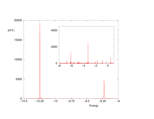
Figure 14: Energy spectrum of the Hubbard model obtained from the simulator. The lattice has $4\times 2$ sites (which requires 16 qubits), with $t_{x}=1$, $t_{y}=1$ and ${\cal U}=4$ and the time steps used in the Trotter approximation (to prepare the initial state and apply the evolution) are $\Delta t_{1}=\Delta t_{2}=0.05$.

The results for the simulation of the Hubbard model are shown in Fig. 14. There, we also show the parameters $\Delta t_{1}$ and $\Delta t_{2}$ corresponding to the time-steps we used in the initial state preparation, where we used a first-order Trotter approximation, and in the time evolution, where we used a second-order Trotter approximation.

In closing this Section we would like to emphasize that the simulation of the Hubbard model by a quantum computer which uses the standard model is just an example. Suppose one wants to simulate the Anderson model bonca instead using the same quantum computer, then similar steps to the ones described above should be followed. (There are two types of fermions but the isomorphism still applies.) Similarly, if one wants to use a different quantum computer which has another natural “language” (i.e., a different operator algebra which therefore represents a different model of computation) one can still apply the ideas developed above simply by choosing the right isomorphism or “dictionary” batista01 .

V Concluding Remarks

We addressed several broad issues associated with the simulation of physical phenomena by quantum networks. We first noted that in quantum mechanics the physical systems we want to simulate are expressed by operators satisfying certain algebras that may differ from the operators and the algebras associated with the physical system representing the quantum network used to do the simulation. We pointed out that rigorous mappings batista01 between these two sets of operators exist and are sufficient to establish the equivalence of the different physical models to a universal model of quantum computation and the equivalence of different physical systems to that model.

We also remarked that these mappings are insufficient for establishing that the quantum network can simulate any physical system efficiently even if the mappings between the systems only involves a polynomial number of steps. We argued that one must also demonstrate the main steps of initialization, evolution, and measurement all scale polynomially with complexity. More is needed than just having a large Hilbert space and inherent parallelism. Further, we noted that some types of measurements important to understanding physical phenomena lack effective quantum algorithms.

In this paper we mainly explored various issues associated with efficient physical simulations by a quantum network, focusing on the construction of quantum network models for such computations. The main questions we addressed were how do we reduce the number of qubits and quantum gates needed for the simulation and how do we increase the amount of physical information measurable. We first summarized the quantum network representation of the standard model of quantum computation, discussing both one and multi-qubit circuits, and then recalled the connection between the spin and fermion representations. We next discussed the initialization, evolution, and measurement processes. In each case we defined procedures simpler than the ones presented in our previous paper sfer , greatly improving the efficiency with which they can be done. We also gave algorithms that greatly expanded the types of measurements now possible. For example, besides certain correlation functions, the spectrum of operators, including the energy operator, is now possible. Our application of this technology to a system of lattice fermions and the construction of a simulator was also discussed and used the Hubbard model as an example. This application gave an explicit example of how the mapping between the operator of the physical system of interest and those of the standard model of quantum computation work. We also gave details of how we implemented the initialization, evolution, and measurement steps of the quantum network on a classical computer, thereby creating an quantum network simulator.

Clearly, a number of challenges for the efficient simulation of physical systems on a quantum network remain. We are prioritizing our research on those issues associated with problems that are extremely difficult for quantum many-body scientists to solve on classical computers. There are no known efficient quantum algorithms for broad spectrum ground-state (zero temperature) and thermodynamics (finite temperature) measurements of correlations in quantum states. These measurements would help establish the phases of those states. Generating those states is itself a difficult task.

Many problems in physics simulation, such as the challenging protein folding problem, are considered to be well modeled by classical physics. Can quantum networks be used to obtain significantly better (more efficient) algorithms for such essentially classical physics problems?

Appendix A Different state preparation

A.1 Coherent State Preparation: An example

Here we illustrate by example the decomposition of an operator of the form $e^{i\vec{a}^{\dagger}M\vec{a}}$ to generate an initial state. Typically $M$ is generated by some mean-field solution to the physical problem of interest. Considerable detail is given.

We consider 2 spinless fermions in a one-dimensional lattice of 4 sites ($N_{e}=2$ , $n=4$). The operators $a_{j}$ and $a^{\dagger}_{j}$ annihilate and create a fermion in the site $j$ of the lattice. We want to prepare an initial state $|{\phi^{\prime}}\rangle=c^{\dagger}_{0}c^{\dagger}_{\pi/2}|{\mbox{vac}}\rangle$ from the state $|{\phi}\rangle=a^{\dagger}_{1}a^{\dagger}_{2}|{\mbox{vac}}\rangle$, where the operators $c_{k}$ and $c^{\dagger}_{k}$ annihilate and create a fermion in the state of wave vector $k$, that is:

$$c^{\dagger}_{k}=\frac{1}{2}\sum\limits_{j=1}^{4}e^{ikx_{j}}a^{\dagger}_{j}\ ,$$ (46)

where $k=0,{\pi/2},{\pi},{3\pi/2}$ are all possible wave vectors of the system, and $x_{j}$ is the position in the lattice of the site (i.e., $x_{j}=j-1$).

From Eq. 46, we see that the state $|{\phi^{\prime}}\rangle$ is a linear combination of states of the form $a^{\dagger}_{i}a^{\dagger}_{j}|{\mbox{vac}}\rangle$. The change of basis $e^{iM}$ (Eq. 21) between the two sets of fermionic operators is:

$$\pmatrix{c_{0}^{\dagger}\cr c_{\pi/2}^{\dagger}\cr c_{\pi}^{\dagger}\cr c_{3\pi/2}^{\dagger}\cr}=\frac{1}{2}\ \pmatrix{1&1&1&1\cr 1&i&-1&-i\cr 1&-1&1&-1\cr 1&-i&-1&i\cr}\ \pmatrix{a_{1}^{\dagger}\cr a_{2}^{\dagger}\cr a_{3}^{\dagger}\cr a_{4}^{\dagger}\cr}\ .$$ (47)

If we calculate the eigenvalues and the eigenvectors of the matrix $e^{iM}$, from Eq. 47 we obtain:

$$e^{iM_{D}}=\ \pmatrix{-1&0&0&0\cr 0&i&0&0\cr 0&0&1&0\cr 0&0&0&1\cr}\ ,$$ (48)

where $M_{D}$ is $M$ in its diagonal form. Then, we have:

$$M_{D}=-i\log(e^{iM_{D}})=\ \pmatrix{\pi&0&0&0\cr 0&\pi/2&0&0\cr 0&0&0&0\cr 0&0&0&0\cr}\ .$$ (49)

To obtain the matrix $M=A^{\dagger}M_{D}A$, we need to know the unitary matrix $A$, which is constructed with the eigenvectors of the matrix $e^{iM}$. In this case we have:

$$A^{\dagger}=\ \pmatrix{-1/2&0&1/\sqrt{2}&1/\sqrt{2}\cr 1/2&-1/\sqrt{2}&1/\sqrt{2}&0\cr 1/2&0&-1/\sqrt{2}&1/\sqrt{2}\cr 1/2&1/\sqrt{2}&1/\sqrt{2}&0\cr}\ ,$$ (50)

hence, the Hermitian matrix $M$ is:

$$M=\frac{\pi}{4}\ \pmatrix{1&-1&-1&-1\cr-1&2&1&0\cr-1&1&1&1\cr-1&0&1&2\cr}\ .$$ (51)

In order to obtain $|{\phi^{\prime}}\rangle$ we prepare the state $|{\phi}\rangle$ and then apply the evolution $U=e^{i\vec{a}^{\dagger}M\vec{a}}$. If we want to simulate this fermionic system in a quantum computer (standard model), we have to use the spin-fermion connection (Section II.3), and write the operator $U$ as a combination of single qubit rotations and two qubit interactions. Also, the initial state $|{\phi}\rangle$ must be written in the standard model:

$$|{\phi}\rangle = a^{\dagger}_{1}a^{\dagger}_{2}|{\mbox{vac}}\rangle=\sigma^{1}_{+}(-\sigma^{1}_{z}\sigma^{2}_{+})|{\widetilde{\mbox{vac}}}\rangle=\sigma^{1}_{+}\sigma^{2}_{+}|{\widetilde{\mbox{vac}}}\rangle$$ (52)

$$= |{0}\rangle_{1}\otimes|{0}\rangle_{2}\otimes|{1}\rangle_{3}\otimes|{1}\rangle_{4}=|{\uparrow\uparrow\downarrow\downarrow}\rangle\ ,$$ (53)

where the vacuum state in the standard model is $|{\widetilde{\mbox{vac}}}\rangle=|{1}\rangle_{1}\otimes|{1}\rangle_{2}\otimes\cdots\otimes|{1}\rangle_{n}=|{\downarrow\downarrow\cdots\downarrow}\rangle$ ($(\prod\limits_{l=1}^{j-1}-{\sigma}_{z}^{l})\sigma_{-}^{j}|{\widetilde{\mbox{vac}}}\rangle=a_{j}|{\mbox{vac}}\rangle=0$). With this mapping, the state $|{\phi^{\prime}}\rangle$ is a linear combination of states of $z$-component of spin 0.

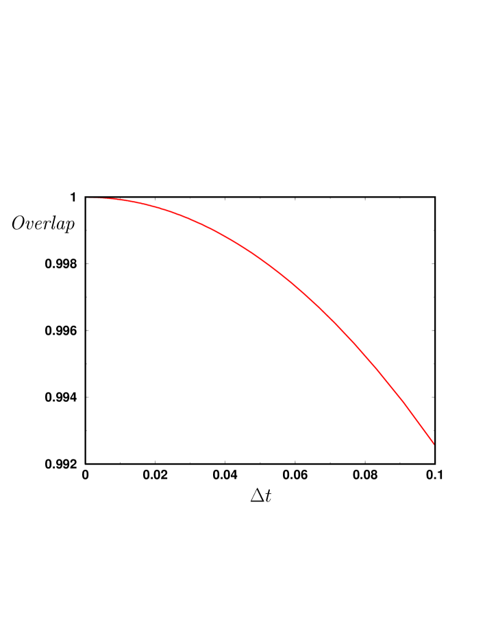
Figure 15: Overlap between the exact initial state and the state prepared with the Trotter decomposition, for a system with two fermions in a 4-sites lattice.

As noted in Section III.2, sometimes the decomposition of the operator $U$ in terms of one and two qubit operations is very difficult. To avoid this problem, we can use the Trotter decomposition (Eq. 23). In Fig. 15 we show the overlap (projection) between the state $|{\phi^{\prime}}\rangle$ and the state prepared using the first-order Trotter decomposition of $U$ applied to the state $|{\phi}\rangle$.

A.2 Jastrow-type Wave Functions

A Jastrow-type wave function is often a better approximation to the actual state of an interacting system, particularly when interactions are strong and short-ranged. Often one varies the parameters in these functions to produce a state that satisfies a variational principle for some physical quantity like the energy. Such states build in correlated many-body effects and are, in general, entangled states. The states described in the previous subsection (Appendix A 1) are unentangled.

The classic form of a Jastrow-type wave function for fermions isblaizot

$$|{\Psi_{0}}\rangle=e^{S}|{\phi^{\prime}}\rangle\ ,$$ (54)

where $S=\sum\limits_{ij}\alpha_{ij}c^{\dagger}_{i}c_{j}^{\;}+\sum\limits_{ijkl}\beta_{ijkl}c^{\dagger}_{i}c^{\dagger}_{j}c_{k}^{\;}c_{l}^{\;}+\cdots$ is an operator which creates particle and hole excitations, and $|{\phi^{\prime}}\rangle$ is typically a Slater determinant. The $N$-body correlations embodied in $S$ take into account the short-range forces not included in $|{\phi^{\prime}}\rangle$. We will assume the $\alpha_{ij}$ and $\beta_{ijkl}$ have been determined by some suitable means (for example, by a coupled-cluster calculation). If we decompose $e^{S}$ into a linear combination of unitary operators, we can then decompose $|{\Psi_{0}}\rangle$ into a linear combination of Slater determinants and thus prepare $|{\Psi_{0}}\rangle$ as explained in sfer . Also, if the coefficients $\alpha_{ij}$ and $\beta_{ijkl}$ are small, we can approximate $e^{S}$ by the first few terms in its Taylor expansion. Again, the state $|{\Psi_{0}}\rangle$ will be a linear combination of Slater determinants.

Obviously, it is more natural for a quantum computer to generate a correlated state of the form

$$|{\Psi_{0}}\rangle=e^{iS}|{\phi^{\prime}}\rangle\ ,$$ (55)

where $e^{iS}$ is a unitary operator. In order to determine the $N$-body correlation coefficients $\alpha_{ij}$ and $\beta_{ijkl}$, one could, in principle, use the technique of unitary transformations introduced by Villars villars .

Appendix B Discrete Fourier Transforms

In practice, to evaluate the discrete Fast Fourier Transform (DFFT) one uses discrete samples, therefore Eq. 31 must be modified accordingly. In Fig. 14 we see that instead of having $\delta$-functions (Dirac’s functions), we have finite peaks in some range of energies, close to the eigenvalues of the Hamiltonian. Accordingly, one cannot determine the eigenvalues with the same accuracy as other numerical calculations. However, there are some methods that give the results more accurately from the DFFT.

As a function of the frequency $\Omega_{m}$, the DFFT ($\tilde{F}(\Omega_{m})$) is given by:

$$\tilde{F}(\Omega_{m})=\Delta t\sum\limits_{j=0}^{N-1}F(t_{j})e^{i\Omega_{m}t_{j}}\ ,$$ (56)

where $t_{j}=j\Delta t$ are the different times at which the function $F$ is sampled (in the case of Section  III.3.4, $F(t_{j})=\langle\hat{U}(t_{j})\rangle$), $\Omega_{m}=\frac{2\pi m}{N\Delta t}$ are the possible frequencies to evaluate the FFT of $F(t)$ and $N$ is the number of samples. ($N$ must be an integer power of 2.)

Since we are interested in $F(t)=\sum\limits_{n=0}^{\cal L}|\gamma_{n}|^{2}\ e^{-i\lambda_{n}t}$ (Eq. 30),

$$\tilde{F}(\Omega_{m})=\Delta t\sum\limits_{n=0}^{\cal L}|\gamma_{n}|^{2}\sum\limits_{j=0}^{N-1}e^{i[\Omega_{m}-\lambda_{n}]t_{j}}\ ,$$ (57)

and then

$$\tilde{F}(\Omega_{m})=\Delta t\sum\limits_{n=0}^{\cal L}|\gamma_{n}|^{2}\ \frac{e^{i(\Omega_{m}-\lambda_{n})\Delta tN}-1}{e^{i(\Omega_{m}-\lambda_{n})\Delta t}-1}\ .$$ (58)

If $\Omega_{m}$ is close to one of the eigenvalues $\lambda_{n}$ and the $\lambda_{n}$ are sufficiently far appart to be well resolved, we can neglect all terms in the sum other than $n$. If we take $\Omega_{m}$ and $\Omega_{m+1}=\Omega_{m}+\frac{2\pi}{N\Delta t}$, both close to $\lambda_{n}$ in such a way that $|\tilde{F}(\Omega_{m})|\gg|\tilde{F}(\Omega_{m+1})|\gg 0$, then from Eq. 58 we find that

$$\frac{\tilde{F}(\Omega_{m+1})}{\tilde{F}(\Omega_{m})}\approx\frac{e^{i(\Omega_{m}-\lambda_{n})\Delta t}-1}{e^{i(\Omega_{m+1}-\lambda_{n})\Delta t}-1}\ .$$ (59)

After simple algebraic manipulations (and approximating $\ln(1+z)\approx z$ for $|z|\rightarrow 0$) we obtain the correction to the energy $\lambda_{n}$:

$$\lambda_{n}=\Omega_{m}+\Delta\lambda_{n}$$ (60)

with

$$\Delta\lambda_{n}\approx{\rm Re}\biggl{[}i\frac{\tilde{F}(\Omega_{m+1})}{\tilde{F}(\Omega_{m})}\Bigl{[}\frac{e^{i2\pi/N}-1}{\Delta t}\Bigr{]}\biggr{]}$$ (61)

Figure 3: (a) Some one qubit elementary gates and (b) a two qubit elementary gate.

References

- (1) G. Ortiz, J.E. Gubernatis, E. Knill, and R. Laflamme, Phys. Rev. A 64, 22319 (2001).
- (2) S. Somaroo, C.-H. Tseng, T. F. Havel, R. Laflamme and D. G. Cory, Phys. Rev. Lett. 82, 5318 (1999).
- (3) C.D. Batista and G. Ortiz, Phys. Rev. Lett. 86, 1082 (2001). C.D. Batista and G. Ortiz, cond-mat/xxxxx.
- (4) B. M. Terhal and D. P. DiVincenzo, Phys. Rev. A 61, 2301 (2000).
- (5) See for instance Quantum Monte Carlo Methods in Condensed-Matter Physics, edited by M. Suzuki (World Scientific, Singapore, 1993); W. M. C. Foulkes, L. Mitas, R. J. Needs, and G. Rajagopal, Rev. Mod. Phys. 73, 33 (2001).
- (6) We thank U.-J. Wiese and S. Chandrasekharan for pointing this out to us.
- (7) E. Farhi, J. Goldstone, S. Gutmann, J. Lapan, A. Lundgren, and D. Preda, Science 292, 472 (2001).
- (8) A. Barenco et al., Phys. Rev. A 52, 3457 (1995).
- (9) D. DiVincenzo, Phys. Rev. A 51, 1015 (1995).
- (10) M. D. Price, S. S. Somaroo, A. E. Dunlop, T. F. Havel, D. G. Cory, Phys. Rev. A 60, 2777 (1999).
- (11) S. S. Somaroo, D. G. Cory, T. F. Havel, Phys. Lett. A 240, 1 (1998).
- (12) S. Bravyi and A. Kitaev, quant-ph/0003137 (2000).
- (13) P. Jordan and E. Wigner, Z. Phys. 47, 631 (1928).
- (14) E. Fradkin, Phys. Rev. Lett. 63, 322 (1989).
- (15) L. Huerta and J. Zanelli, Phys. Rev. Lett. 71, 3622 (1993).
- (16) J.-P. Blaizot and G. Ripka, Quantum Theory of Finite Systems, (MIT Press, Cambridge, 1986).
- (17) A. Perelomov, Generalized Coherent States and their Applications (Springer-Verlag, Berlin, 1986).
- (18) For a brief review, see M. Suzuki, in Quantum Monte Carlo Methods in Condensed-Matter Physics, edited by M. Suzuki (World Scientific, Singapore, 1993), pg. 1.
- (19) C. Miquel, J. P. Paz, M. Saraceno, E. Knill, R. Laflamme and C. Negrevergne, unpublished manuscript (2001).
- (20) A. Yu Kitaev, quant-ph/9511026 (1995).
- (21) R. Cleve, A. Ekert, C. Macchiavello and M. Mosca, Proc. R. Soc. Lond. A 454, 339 (1998).
- (22) D. S. Abrams and S. Lloyd, Phys. Rev. Lett. 83, 5162 (1999).
- (23) J. W. Negele and H. Orland, Quantum Many-Particle Systems (Addison-Wesley, Redwood City, 1988).
- (24) See for instance J. Bona and J. E. Gubernatis, Phys. Rev. B 58, 6992 (1998).
- (25) F. Villars, in Proceedings of the International School of Physics “Enrico Fermi”, Course XXIII: Nuclear Physics, edited by V.F. Weisskopf (Academic Press, New York, 1963), pg. 1.