A simple model of quantum trajectories

Abstract

Quantum trajectory theory, developed largely in the quantum optics community to describe open quantum systems subjected to continuous monitoring, has applications in many areas of quantum physics. In this paper I present a simple model, using two-level quantum systems (q-bits), to illustrate the essential physics of quantum trajectories and how different monitoring schemes correspond to different “unravelings” of a mixed state master equation. I also comment briefly on the relationship of the theory to the Consistent Histories formalism and to spontaneous collapse models.

I Introduction

Over the last ten years the theory of quantum trajectories has been developed by a wide variety of authors [1, 2, 3, 4, 5, 6, 7, 8] for a variety of purposes, including the ability to model continuously monitored open systems [1, 3, 4], improved numerical calculation [2, 8], and insight into the problem of quantum measurement [5, 6, 7]. However, outside the small communities of quantum optical theory and quantum foundations, the theory remains little known and poorly understood.

Indeed, the association with quantum foundations has convinced many observers that quantum trajectory theory is different from standard quantum mechanics, and therefore to be regarded with deep suspicion [9]. While it is true that stochastic Schrödinger and master equations of the type treated in quantum trajectories are sometimes postulated in alternative quantum theories [10, 11, 12, 13], these same types of equations arise quite naturally in describing quantum systems interacting with environments (open systems) which are subjected to monitoring by measuring devices. In these systems, the stochastic equations arise as effective evolution equations, and are in no sense anything other than standard quantum mechanics (except, perhaps, in the trivial sense of approaching the limit of continuous measurement).

The fact that this is not widely appreciated, even in fields which might usefully employ quantum trajectories, is a great pity. I attribute it to confusion about exactly what the theory is, and how these equations arise.

To combat this confusion I present in this paper a simple model for quantum trajectories, using only two-level quantum systems (quantum bits or q-bits). Because of the recent interest in quantum information a great deal of attention has been paid to the possible interactions and measurements of two-level systems; I will draw on this to build my model and show how effective stochastic evolution equations can arise due to a system interacting with a continuously monitored environment.

This paper is intended as a tutorial, giving the physical basis of quantum trajectories without the complications arising from realistic systems and environments. As an aid in understanding or teaching the material, I have included a number of exercises throughout this paper. For the most part these involve working out derivations which arise in developing the model, but which are not crucial for following the main argument. The solutions to the exercises are included in the appendix.

A The model

For simplicity, I will consider the simplest possible quantum system: a single two-level atom or q-bit. The environment will also consist of q-bits. While this is far easier to analyze than the more complicated systems used in most actual quantum trajectory simulations, it can illustrate almost all of the phenomena which occur in more realistic cases. Moreover, the recent interest in quantum computation and quantum information has spurred a great deal of work on such systems of q-bits, which we can draw on.

I will assume that the environment bits interact with the system bit successively for finite, disjoint intervals. I will further assume that these bits are all initially in the same state, have no correlations with each other, and do not interact amongst themselves. (See figure 1.) Therefore all that we need to consider is a succession of interactions between two q-bits. After each environment bit interacts with the system, we can measure it in any way we like, and use the information obtained to update our knowledge of the state.

This model of system and environment may seem excessively abstract, but in fact a number of experimental systems can be approximated in this way. For instance, in experiments with ions in traps, residual molecules of gas can occasionally pass close to the ion, perturbing its internal state. In cavity QED experiments the system might be an electromagnetic mode inside a high-$Q$ cavity. If there is never more than a single photon present, the mode is reasonably approximated as a two-level system. This mode can be probed by sending Rydberg atoms through the cavity one at a time in a superposition of two neighboring electronic states, and measuring the atoms’ electronic states upon their emergence. In this case, the atoms are serving as both an environment for the cavity mode and a measurement probe. Similarly, in an optical microcavity the external electromagnetic field can be thought of as a series of incoming waves which are reflected by the cavity walls; photons leaking out from the cavity can move these modes from the vacuum to the first excited state. (See figure 2.)

B Plan of this paper

In section 2, I describe systems of q-bits, and the possible two-bit interactions they can undergo. In section 3, I examine possible kinds of measurements, including positive operator valued and weak measurements.

In section 4, I present the model of the system and environment. In section 5 I show how it is possible to give an effective evolution for the system alone by tracing out the environment degrees of freedom, producing a kind of master equation.

In section 6, I consider the effects on the system state of a measurement on the environment, and deduce stochastic evolution equations for the system state, conditioned on the random outcome of the environment measurements.

In sections 7–8, I examine different interactions and measurements, and how they lead to different effective evolution equations for pure states—a kind of stochastic Schrödinger equation. I show how under some circumstances the system appears to evolve by large discontinuous jumps, while for other models the state undergoes a slow diffusion in Hilbert space. I further show that by averaging over the different measurement outcomes we recover the master equation evolution of section 5.

In section 9, I consider measurement schemes which give only partial information about the system. These schemes lead to stochastic master equations rather than Schrödinger equations.

Finally, in section 10 I relax the assumption of measurement, and discuss how quantum trajectories can be used to give insight into the nature of measurement itself, using the decoherent (Consistent) histories formulation of quantum mechanics. I also briefly consider alternative quantum theories which make use of stochastic equations. In section 11 I summarize the paper and draw conclusions. I present the solution to the exercises in the appendix.

II Two-level systems and their interactions

The simplest possible quantum mechanical system is a two-level atom or q-bit, which has a two-dimensional Hilbert space ${\cal H}_{2}$. There are many physical embodiments of such a system: the spin of a spin-1/2 particle, the polarization states of a photon, two hyperfine states of a trapped atom or ion, two neighboring levels of a Rydberg atom, the presence or absence of a photon in a microcavity, etc. All of the above have been proposed in various schemes for quantum information and quantum computation, and many have been used in actual experiments. (For a good general source on quantum computation and information, see Nielsen and Chuang [14] and references therein.)

By convention, we choose a particular basis and label its basis states ${|0\rangle}$ and ${|1\rangle}$, which we define to be the eigenstates of the Pauli spin matrix ${\hat{\sigma}_{z}}$ with eigenvalues $-1$ and $+1$, respectively. We similarly define the other Pauli operators ${\hat{\sigma}_{x}},{\hat{\sigma}_{y}}$; linear combinations of these, together with the identity ${\hat{1}}$, are sufficient to produce any operator on a single q-bit.

The most general pure state of a q-bit is

$${|\psi\rangle}=\alpha{|0\rangle}+\beta{|1\rangle},\ \ |\alpha|^{2}+|\beta|^{2}=1\;.$$ (1)

A global phase may be assigned arbitrarily, so all physically distinct pure states of a single q-bit form a two-parameter space. A useful parametrization is in terms of two angular variables $\theta$ and $\phi$,

$${|\psi\rangle}=\cos(\theta/2){\rm e}^{-i\phi/2}{|0\rangle}+\sin(\theta/2){\rm e}^{i\phi/2}{|1\rangle}\;,$$ (2)

where $0\leq\theta\leq\pi$ and $0\leq\phi\leq 2\pi$. These two parameters define a point on the Bloch sphere. The north and south poles of the sphere represent the eigenstates of ${\hat{\sigma}_{z}}$, and the eigenstates of ${\hat{\sigma}_{x}}$ and ${\hat{\sigma}_{y}}$ lie on the equator. Orthogonal states always lie opposite each other on the sphere.

If we allow states to be mixed, we represent a q-bit by a density matrix $\rho$; the most general density matrix can be written

$$\rho=p{|\psi\rangle}{\langle\psi|}+(1-p){|\bar{\psi}\rangle}{\langle\bar{\psi}|}\;,$$ (3)

where ${|\psi\rangle}$ and ${|\bar{\psi}\rangle}$ are two orthogonal pure states, ${\langle\psi|\bar{\psi}\rangle}=0$. The mixed states of a q-bit form a three parameter family:

$$\rho = \left({1+r\over 2}\cos^{2}(\theta/2)+{1-r\over 2}\sin^{2}(\theta/2)\right){|0\rangle}{\langle 0|}+$$ (6)

$$\left({1+r\over 2}\sin^{2}(\theta/2)+{1-r\over 2}\cos^{2}(\theta/2)\right){|1\rangle}{\langle 1|}+$$

$$r\cos(\theta/2)\sin(\theta/2)\left({\rm e}^{i\phi}{|0\rangle}{\langle 1|}+{\rm e}^{-i\phi}{|1\rangle}{\langle 0|}\right)\;,$$

where $\theta,\phi$ are the same angular parameters as before and $0\leq r\leq 1$. The limit $r=1$ is the set of pure states, parametrized as in (2), while $r=0$ is the completely mixed state $\rho={\hat{1}}/2$. Thus we can think of the Bloch sphere as having pure states on its surface and mixed states in its interior; and the distance $r$ from the center is a measure of the state’s purity. It is simply related to the parameter $p$ in (3): $p=(1+r)/2$, $1-p=(1-r)/2$.

For two q-bits, the Hilbert space ${\cal H}_{2}\otimes{\cal H}_{2}$ has a tensor-product basis

$${|0\rangle}_{A}\otimes{|0\rangle}_{B} \equiv {|00\rangle}_{AB}\;,$$ (7)

$${|0\rangle}_{A}\otimes{|1\rangle}_{B} \equiv {|01\rangle}_{AB}\;,$$ (8)

$${|1\rangle}_{A}\otimes{|0\rangle}_{B} \equiv {|10\rangle}_{AB}\;,$$ (9)

$${|1\rangle}_{A}\otimes{|1\rangle}_{B} \equiv {|11\rangle}_{AB}\;;$$ (10)

similarly, for $N$ q-bits we can define a basis $\{{|i_{N-1}i_{N-2}\cdots i_{0}\rangle}\}$, $i_{k}=0,1$. A useful labeling of these $2^{N}$ basis vectors is by the integers $0\leq j<2^{N}$ whose binary expressions are $i_{N-1}\cdots i_{0}$:

$${|j\rangle}\equiv{|i_{N-1}\cdots i_{0}\rangle},\ \ j=\sum_{k=0}^{N-1}i_{k}2^{k}\;.$$ (11)

All states evolve according to the Schrödinger equation with some Hamiltonian ${\hat{H}}(t)$,

$${d{|\psi\rangle}\over dt}=-{i\over\hbar}{\hat{H}}(t){|\psi\rangle}.$$ (12)

Over a finite time this is equivalent to applying a unitary operator ${\hat{U}}$ to the state ${|\psi\rangle}$,

$${\hat{U}}={\rm T:}\exp\left\{-{i\over\hbar}\int_{t_{0}}^{t_{f}}dt\,{\hat{H}}(t)\right\}:\;.$$ (13)

where ${\rm T:}:$ indicates that the integral should be taken in a time-ordered sense, with early to late times being composed from right to left. For the models I consider in this paper I will treat all time evolution at the level of unitary transformations rather than explicitly solving the Schrödinger equation, so time can be treated as a discrete variable

$${|\psi_{n}\rangle}={\hat{U}}_{n}{\hat{U}}_{n-1}\cdots{\hat{U}}_{1}{|\psi_{0}\rangle}\;.$$ (14)

For a mixed state $\rho$, Schrödinger time evolution is equivalent to $\rho\rightarrow{\hat{U}}\rho{\hat{U}^{\dagger}}$. Henceforth, I will also assume $\hbar=1$.

If the unitary operator ${\hat{U}}_{n}$ is weak, that is, close to the identity, one can always find a Hamiltonian operator ${\hat{H}}_{n}$ such that

$${\hat{U}}_{n}=\exp\left\{-i{\hat{H}}_{n}\delta t\right\}\approx 1-i{\hat{H}}_{n}\delta t\;.$$ (15)

Thus, one can easily recover the Schrödinger equation from a description in terms of unitary operators,

$$\delta{|\psi_{n}\rangle}={|\psi_{n}\rangle}-{|\psi_{n-1}\rangle}=({\hat{U}}_{n}-{\hat{1}}){|\psi_{n-1}\rangle}=-i{\hat{H}}_{n}{|\psi_{n-1}\rangle}\delta t\;.$$ (16)

Exercise 1. Show that the most general unitary operator on a single q-bit can be written

$${\hat{U}}={\hat{1}}\cos\varphi+i{\vec{n}}\cdot{\hat{\vec{\sigma}}}\sin\varphi=\exp\{i\varphi{\vec{n}}\cdot{\hat{\vec{\sigma}}}\}\;,$$ (17)

modulo an irrelevant overall phase, where ${\vec{n}}=\{n_{x},n_{y},n_{z}\}$ is a three-vector with unit norm and ${\hat{\vec{\sigma}}}=\{{\hat{\sigma}_{x}},{\hat{\sigma}_{y}},{\hat{\sigma}_{z}}\}$. In the Bloch sphere picture this is a rotation by an angle $\varphi$ about the axis defined by ${\vec{n}}$, with three real parameters (four if one includes the global phase).

For two q-bits there is unfortunately no such simple visualization as the Bloch sphere. However, to specify any unitary transformation it suffices to give its effect on a complete set of basis vectors. I will consider only a fairly limited set of two-bit transformations in this paper, and no transformations involving more than two q-bits, but the simple formalism I derive readily generalizes to higher-dimensional systems.

Let us examine a couple of examples of two-bit transformations. The controlled-NOT gate (or CNOT) is widely used in quantum computation; applied to the tensor-product basis vectors it gives

$${\hat{U}}_{\rm CNOT}{|00\rangle} = {|00\rangle}\;,$$ (18)

$${\hat{U}}_{\rm CNOT}{|01\rangle} = {|01\rangle}\;,$$ (19)

$${\hat{U}}_{\rm CNOT}{|10\rangle} = {|11\rangle}\;,$$ (20)

$${\hat{U}}_{\rm CNOT}{|11\rangle} = {|10\rangle}\;,$$ (21)

or in matrix form

$${\hat{U}}_{\rm CNOT}=\left(\matrix{1&0&0&0\cr 0&1&0&0\cr 0&0&0&1\cr 0&0&1&0\cr}\right)\;.$$ (22)

If the first bit is in state ${|0\rangle}$ this gate leaves the second bit unchanged; if the first bit is in state ${|1\rangle}$ the second bit is flipped ${|0\rangle}\leftrightarrow{|1\rangle}$. Hence the name: whether a NOT gate is performed on the second bit is controlled by the first bit. In terms of single-bit operators this is ${\hat{U}}_{\rm CNOT}={|0\rangle}{\langle 0|}\otimes{\hat{1}}+{|1\rangle}{\langle 1|}\otimes{\hat{\sigma}_{x}}$.

Another important gate in quantum computation is the SWAP; applied to the tensor-product basis vectors it gives

$${\hat{U}}_{\rm SWAP}{|00\rangle} = {|00\rangle}\;,$$ (23)

$${\hat{U}}_{\rm SWAP}{|01\rangle} = {|10\rangle}\;,$$ (24)

$${\hat{U}}_{\rm SWAP}{|10\rangle} = {|01\rangle}\;,$$ (25)

$${\hat{U}}_{\rm SWAP}{|11\rangle} = {|11\rangle}\;,$$ (26)

which in matrix form is just

$${\hat{U}}_{\rm SWAP}=\left(\matrix{1&0&0&0\cr 0&0&1&0\cr 0&1&0&1\cr 0&0&0&1\cr}\right)\;.$$ (27)

As the name suggests, the SWAP gate just exchanges the states of the two bits: ${\hat{U}}_{\rm SWAP}({|\psi\rangle}\otimes{|\phi\rangle})={|\phi\rangle}\otimes{|\psi\rangle}$.

CNOT and SWAP are examples of two-bit quantum gates. Such gates are of tremendous importance in the theory of quantum computation. These two gates in particular have an additional useful property. Note that the operator ${\hat{U}}_{\rm CNOT}={\hat{U}^{\dagger}}_{\rm CNOT}$, i.e., it is both unitary and Hermitian. This is also true of ${\hat{U}}_{\rm SWAP}$. This is only possible if all of the operator’s eigenvalues are $1$ or $-1$. This also means that these operators are their own inverses, ${\hat{U}}^{2}_{\rm CNOT}={\hat{U}}^{2}_{\rm SWAP}={\hat{1}}$. (Among single-bit operators, the Pauli matrices ${\hat{\sigma}}_{x,y,z}$ also have this property, as does any operator ${\vec{n}}\cdot{\hat{\vec{\sigma}}}$.)

This property of being both unitary and Hermitian makes it possible to define one-parameter families of two-bit unitary transformations:

$${\hat{U}}_{\rm CNOT}(\theta) = \exp\left\{-i\theta{\hat{U}}_{\rm CNOT}\right\}$$ (28)

$$= {\hat{1}}\cos\theta-i{\hat{U}}_{\rm CNOT}\sin\theta\;,$$ (29)

and similarly

$${\hat{U}}_{\rm SWAP}(\theta) = \exp\left\{-i\theta{\hat{U}}_{\rm SWAP}\right\}$$ (30)

$$= {\hat{1}}\cos\theta-i{\hat{U}}_{\rm SWAP}\sin\theta\;.$$ (31)

Exercise 2. Show that any operator ${\hat{U}}$ which is both unitary and Hermitian satisfies $\exp(-i\theta{\hat{U}})={\hat{1}}\cos\theta-i{\hat{U}}\sin\theta$.

These families range from the identity ${\hat{1}}$ for $\theta=0$ to the full CNOT (or SWAP) gate for $\theta=\pi/2$, up to a global phase. For small values $\theta\ll 1$, this is a weak interaction, which leaves the state only slightly altered.

These families do have an undesirable characteristic, however. Suppose we apply ${\hat{U}}_{\rm CNOT}(\theta)$ to a two-bit state of the form $(\alpha{|0\rangle}+\beta{|1\rangle})\otimes{|\psi\rangle}$. The new state is

$${\hat{U}}_{\rm CNOT}(\theta)(\alpha{|0\rangle}+\beta{|1\rangle})\otimes{|\psi\rangle} = (\alpha{\rm e}^{-i\theta}{|0\rangle}+\beta\cos\theta{|1\rangle})\otimes{|\psi\rangle}$$ (33)

$$-i\beta\sin\theta{|1\rangle}\otimes({\hat{\sigma}_{x}}{|\psi\rangle})\;.$$

This relative phase ${\rm e}^{i\theta}$ between ${|0\rangle}$ and ${|1\rangle}$ is a complication in the calculations that will follow. To avoid this problem, instead of ${\hat{U}}_{\rm CNOT}(\theta)$ and ${\hat{U}}_{\rm SWAP}(\theta)$ we will use interactions of the form ${\hat{Z}}_{A}(\theta){\hat{U}}_{\rm CNOT}(\theta)$, where ${\hat{Z}}_{A}(\theta)=(\exp(-i{\hat{\sigma}_{z}}\theta/2)\otimes{\hat{1}})$, and similarly for ${\hat{U}}_{\rm SWAP}$. The single-bit rotation exactly undoes the extra relative phase produced by ${\hat{U}}_{\rm CNOT}(\theta)$, while changing nothing else.

Before leaving the topic of two-bit gates, I should point out another representation which is sometimes useful. Any operator on two q-bits can formally be written

$${\hat{O}}=\sum_{i,j=0}^{3}R_{ij}\hat{\sigma}_{i}\otimes\hat{\sigma}_{j},$$ (34)

where $\hat{\sigma}_{0}\equiv{\hat{1}}$, $\hat{\sigma}_{1,2,3}\equiv\hat{\sigma}_{x,y,z}$. The matrix elements can be calculated using the identity

$$R_{ij}={\rm Tr}\left\{{\hat{O}}(\sigma_{i}\otimes\sigma_{j})\right\}\;.$$ (35)

If ${\hat{O}}={\hat{O}^{\dagger}}$ is Hermitian, the matrix elements $R_{ij}$ will be real.

If we write the CNOT in this form, it gives matrix elements $R_{ij}$

$${\bf R}_{\rm CNOT}=\left(\matrix{1/2&1/2&0&0\cr 0&0&0&0\cr 0&0&0&0\cr-1/2&1/2&0&0\cr}\right)\;.$$ (36)

Similarly, if we write the SWAP gate this way it has matrix elements

$${\bf R}_{\rm SWAP}=\left(\matrix{1/2&0&0&0\cr 0&1/2&0&0\cr 0&0&1/2&0\cr 0&0&0&1/2\cr}\right)\;.$$ (37)

III Strong and weak measurements

A Projective measurements

In the standard description of quantum mechanics, observables are identified with Hermitian operators ${\hat{O}}={\hat{O}^{\dagger}}$. A measurement returns an eigenvalue $o_{n}$ of ${\hat{O}}$ and leaves the system in the corresponding eigenstate ${|\phi_{n}\rangle}$, ${\hat{O}}{|\phi_{n}\rangle}=o_{n}{|\phi_{n}\rangle}$, with probability $p_{n}=|{\langle\phi_{n}|\psi\rangle}|^{2}$. If a particular eigenvalue is degenerate, one instead uses the projector ${\hat{\cal P}}_{n}$ onto the eigenspace with eigenvalue $o_{n}$; the probability of the measurement outcome is then $p_{n}={\langle\psi|}{\hat{\cal P}}_{n}{|\psi\rangle}$ and the system is left in the state ${\hat{\cal P}}_{n}{|\psi\rangle}/\sqrt{p_{n}}$. For a mixed state $\rho$ the probability of outcome $n$ is $p_{n}={\rm Tr}\{{\hat{\cal P}}_{n}\rho\}$ and the state after the measurement is ${\hat{\cal P}}_{n}\rho{\hat{\cal P}}_{n}/p_{n}$.

Because two observables with the same eigenspaces are completely equivalent to each other (as far as measurement probabilities and outcomes are concerned), we will not worry about the exact choice of Hermitian operator ${\hat{O}}$; instead, we will choose a complete set of orthogonal projections $\{{\hat{\cal P}}_{n}\}$ which represent the possible measurement outcomes. These satisfy

$${\hat{\cal P}}_{n}{\hat{\cal P}}_{n^{\prime}}={\hat{\cal P}}_{n}\delta_{nn^{\prime}}\;,\ \ \sum_{n}{\hat{\cal P}}_{n}={\hat{1}}\;.$$ (38)

A set of projection operators which obey (38) is often referred to as an orthogonal decomposition of the identity. For a single q-bit, the only nontrivial measurements have exactly two outcomes, which we label $+$ and $-$, with probabilities $p_{+}$ and $p_{-}$ and associated projectors of the form

$${\hat{\cal P}}_{\pm}={{\hat{1}}\pm{\vec{n}}\cdot{\hat{\vec{\sigma}}}\over 2}={|\psi_{\pm}\rangle}{\langle\psi_{\pm}|}\;;$$ (39)

this is equivalent to choosing an axis $\vec{n}$ on the Bloch sphere and projecting the state onto one of the two opposite points. All such operators are projections onto pure states. The two projectors sum to the identity operator, ${\hat{\cal P}}_{+}+{\hat{\cal P}}_{-}={\hat{1}}$. The average information obtained from a projective measurement on a q-bit is just the Shannon entropy for the two measurement outcomes,

$$S_{\rm meas}=-p_{+}\log_{2}p_{+}-p_{-}\log_{2}p_{-}\;.$$ (40)

The maximum information gain is precisely one bit, when $p_{+}=p_{-}=1/2$, and the minimum is zero bits when either $p_{+}$ or $p_{-}$ is 0. After the measurement, the state is left in an eigenstate of ${\hat{\cal P}}_{\pm}$, so repeating the measurement will result in the same outcome. This repeatability is one of the most important features of projective measurements.

B Positive operator valued and weak measurements

While projective measurements are the most familiar from introductory quantum mechanics, there is a more general notion of measurement, the positive operator valued measurement (POVM) [15]. Instead of giving a set of projectors which sum to the identity, we give a set of positive operators ${\hat{E}}_{n}$ which sum to the identity:

$$\sum_{n}{\hat{E}}_{n}={\hat{1}}\;.$$ (41)

The probability of outcome $n$ is $p_{n}={\langle\psi|}{\hat{E}}_{n}{|\psi\rangle}$, or for a mixed state $p_{n}={\rm Tr}\{{\hat{E}}_{n}\rho\}$. Unlike a projective measurement, knowing the operators ${\hat{E}}_{n}$ is not sufficient to determine the state of the system after measurement. One must further know a set of operators ${\hat{A}}_{nk}$ such that

$${\hat{E}}_{n}=\sum_{k}{\hat{A}^{\dagger}}_{nk}{\hat{A}}_{nk}\;.$$ (42)

After measurement outcome $n$ the state is

$$\rho\rightarrow\rho^{\prime}=(1/p_{n})\sum_{k}{\hat{A}}_{nk}\rho{\hat{A}^{\dagger}}_{nk}\;.$$ (43)

This measurement will not preserve the purity of states, in general, unless there is only a single ${\hat{A}}_{nk}$ for each ${\hat{E}}_{n}$ (that is, ${\hat{E}}_{n}={\hat{A}^{\dagger}}_{n}{\hat{A}}_{n}$), in which case ${|\psi^{\prime}\rangle}={\hat{A}}_{n}{|\psi\rangle}/\sqrt{p_{n}}$.

Because the positive operators ${\hat{E}}_{n}$ need not be projectors, one is not limited to only two possible outcomes; indeed, there can be an unlimited number of possible outcomes. However, if a POVM is repeated, the same result will not necessarily be obtained the second time. Projective measurements are clearly a special case of POVMs in which results are repeatable. Most actual experiments do not correspond to projective measurements, but are described by some more general POVM.

Conversely, it is easy to show that any POVM can be performed by allowing the system which is to be measured to interact with an additional system, or ancilla, and then doing a projective measurement on the ancilla. In this viewpoint, only some of the information obtained comes from the system; part can also come from the ancilla, which injects extra randomness into the result. This mathematical identification should not be pushed too far, however; in practice, trying to interpret a POVM as a projective measurement on an ancilla often adds complexity without improving understanding.

A particularly interesting kind of POVM for the present purpose is the weak measurement [16]. This is a measurement which gives very little information about the system on average, but also disturbs the state very little.

Loosely speaking, there are two ways a measurement can be considered weak. Suppose we have a q-bit in a state of form (1), and we perform a POVM with the following two operators:

$${\hat{E}}_{0} \equiv {|0\rangle}{\langle 0|}+(1-\epsilon){|1\rangle}{\langle 1|}={\hat{A}}_{0}^{2}\;,$$ (44)

$${\hat{E}}_{1} \equiv \epsilon{|1\rangle}{\langle 1|}={\hat{A}}_{1}^{2}\;,$$ (45)

$${\hat{A}}_{0} \equiv {|0\rangle}{\langle 0|}+\sqrt{1-\epsilon}{|1\rangle}{\langle 1|}\;,$$ (46)

$${\hat{A}}_{1} \equiv \sqrt{\epsilon}{|1\rangle}{\langle 1|}\;,$$ (47)

where $\epsilon\ll 1$. Clearly ${\hat{E}}_{0}$ and ${\hat{E}}_{1}$ are positive and ${\hat{E}}_{0}+{\hat{E}}_{1}={\hat{1}}$, so this is a POVM. The probability $p_{0}={\langle\psi|}{\hat{E}}_{0}{|\psi\rangle}=1-\epsilon|\beta|^{2}$ of outcome 0 is close to 1, while $p_{1}={\langle\psi|}{\hat{E}}_{1}{|\psi\rangle}=\epsilon|\beta|^{2}$ is very unlikely. Thus, most such measurements will give outcome 0, and very little information is obtained about the system.

Exercise 3. Show that the average information gain from this measurement (in bits) is

$$S_{\rm meas}\approx\epsilon|\beta|^{2}(1/\ln 2-\log_{2}\epsilon|\beta|^{2})\ll 1\;.$$ (48)

The state changes very slightly after a measurement outcome 0, with ${|0\rangle}$ becoming slightly more likely relative to ${|1\rangle}$. The new state is

$${|\psi_{0}\rangle}={\hat{A}}_{0}{|\psi\rangle}/\sqrt{p_{0}}=(\alpha{|0\rangle}+\beta\sqrt{1-\epsilon}{|1\rangle})/\sqrt{p_{0}}\;.$$ (49)

However, after an outcome of 1, the state can change dramatically: a measurement outcome of 1 leaves the q-bit in the state ${|1\rangle}$. We see that this type of measurement is weak in that it usually gives little information, and has little effect on the state; but on rare occasions it can give a great deal of information and have a large effect.

By contrast, consider the following positive operators:

$${\hat{E}}_{0} \equiv \left({1+\epsilon\over 2}\right){|0\rangle}{\langle 0|}+\left({1-\epsilon\over 2}\right){|1\rangle}{\langle 1|}={\hat{A}}_{0}^{2}\;,$$ (50)

$${\hat{E}}_{1} \equiv \left({1-\epsilon\over 2}\right){|0\rangle}{\langle 0|}+\left({1+\epsilon\over 2}\right){|1\rangle}{\langle 1|}={\hat{A}}_{1}^{2}\;,$$ (51)

$${\hat{A}}_{0} \equiv \sqrt{1+\epsilon\over 2}{|0\rangle}{\langle 0|}+\sqrt{1-\epsilon\over 2}{|1\rangle}{\langle 1|}\;,$$ (52)

$${\hat{A}}_{1} \equiv \sqrt{1-\epsilon\over 2}{|0\rangle}{\langle 0|}+\sqrt{1+\epsilon\over 2}{|1\rangle}{\langle 1|}\;.$$ (53)

These operators also constitute a POVM. Both ${\hat{E}}_{0}$ and ${\hat{E}}_{1}$ are close to ${\hat{1}}/2$, and so are almost equally likely for all states, $p_{0}\approx p_{1}\approx 1/2$; the information acquired is approximately one bit. But the state of the system is almost unchanged for both outcomes, with the new state being ${|\psi_{j}\rangle}={\hat{A}}_{j}{|\psi\rangle}/\sqrt{p_{j}}$,

$${|\psi_{0}\rangle} = {1\over\sqrt{1+\epsilon(|\alpha|^{2}-|\beta|^{2})}}\left(\alpha\sqrt{1+\epsilon}{|0\rangle}+\beta\sqrt{1-\epsilon}{|1\rangle}\right)$$ (54)

$$\approx \alpha(1+\epsilon|\beta|^{2}){|0\rangle}+\beta(1-\epsilon|\alpha|^{2}){|1\rangle}\;,$$ (55)

$${|\psi_{1}\rangle} = {1\over\sqrt{1-\epsilon(|\alpha|^{2}-|\beta|^{2})}}\left(\alpha\sqrt{1-\epsilon}{|0\rangle}+\beta\sqrt{1+\epsilon}{|1\rangle}\right)$$ (56)

$$\approx \alpha(1-\epsilon|\beta|^{2}){|0\rangle}+\beta(1+\epsilon|\alpha|^{2}){|1\rangle}\;,$$ (57)

for outcomes 0 and 1, respectively. For this type of weak measurement, the measurement outcome is almost random, but does include a tiny amount of information about the state. By performing repeated weak measurements and examining the statistics of the results, one can in effect perform a strong measurement; for the particular case considered here, the state will tend to drift towards either ${|0\rangle}$ or ${|1\rangle}$ with overall probabilities $|\alpha|^{2}$ and $|\beta|^{2}$.

We will see below specific instances of how a POVM can arise by the interaction of the measured system with an ancilla, and the subsequent projective measurement of the ancilla. Quantum trajectories are closely related to such indirect measurement schemes.

IV System and environment

In discussing quantum evolution it is usually assumed that the quantum system is very well isolated from the rest of the world. This is a useful idealization, but it is rarely realized in practice, even in the laboratory. In fact, most systems interact at least weakly with external degrees of freedom [17, 18].

One way of taking this into account is to include a model of these external degrees of freedom in our description. Let us assume that in addition to the system in state ${|\psi\rangle}$ in Hilbert space ${\cal H}_{S}$ with Hamiltonian ${\hat{H}}_{S}$, there is an external environment in state ${|E\rangle}\in{\cal H}_{E}$ with Hamiltonian ${\hat{H}}_{E}$. The joint Hilbert space of the system and environment is the tensor product space ${\cal H}_{S}\otimes{\cal H}_{E}$, and the full Hamiltonian can be written

$${\hat{H}}={\hat{H}}_{S}\otimes{\hat{1}}_{E}+{\hat{1}}_{S}\otimes{\hat{H}}_{E}+{\hat{H}}_{I}\;,$$ (58)

where ${\hat{H}}_{I}$ is a Hamiltonian giving the interaction between the two. The system and environment evolve according to the Schrödinger equation (12) with this full Hamiltonian. Because of the presence of the ${\hat{H}}_{I}$ term, in general even initial product states ${|\psi\rangle}\otimes{|E\rangle}$ will evolve into states which cannot be written as product states:

$${|\psi\rangle}\otimes{|E\rangle}\rightarrow{|\Psi\rangle}=\sum_{j}{|\psi_{j}\rangle}\otimes{|E_{j}\rangle}\;.$$ (59)

Such states are called entangled. If the system and environment are entangled, it is no longer possible to attribute a unique pure state to the system (or environment) alone. The best that can be done is to describe the system as being in a mixed state $\rho_{\rm sys}$, which is the partial trace of the joint state ${|\Psi\rangle}$ over the environment degrees of freedom:

$$\rho_{\rm sys} = {\rm Tr}_{\rm env}\left\{{|\Psi\rangle}{\langle\Psi|}\right\}$$ (60)

$$= \sum_{j,j^{\prime},k}{|\psi_{j}\rangle}{\langle\psi_{j^{\prime}}|}{\langle e_{k}|E_{j}\rangle}{\langle E_{j^{\prime}}|e_{k}\rangle}$$ (61)

$$= \sum_{j,j^{\prime}}{|\psi_{j}\rangle}{\langle\psi_{j^{\prime}}|}{\langle E_{j^{\prime}}|E_{j}\rangle}\;,$$ (62)

where the $\{{|e_{k}\rangle}\}$ are some complete set of orthonormal basis vectors on the environment Hilbert space ${\cal H}_{E}$.

The entanglement of a state can be quantified. The most widely used measure for pure states is the entropy of entanglement. For a system and environment in a joint pure state, this is

$$S_{E}=-{\rm Tr}\{\rho_{S}\log_{2}\rho_{S}\}\;,$$ (63)

which is the von Neumann entropy of the reduced density operator $\rho_{S}$. This entropy is maximized by the density operator $\rho_{S}={\hat{1}}_{S}/{\rm Tr}_{\rm sys}\{{\hat{1}}_{S}\}$; such a density operator is called maximally mixed, and the joint pure state which gives rise to it is called maximally entangled.

Exercise 4. Show that the von Neumann entropy is maximized for $\rho={\hat{1}}/{\rm Tr}\{{\hat{1}}\}.$

Systems which interact with their environments are said to be open. Most real physical environments are extremely complicated, and the interactions between systems and environments are often poorly understood. In analyzing open systems, one often makes the approximation of assuming a simple, analytically solvable form for the environment degrees of freedom.

For the models of this paper, I will assume that both the system and the environment consist solely of q-bits. I will also assume a simple form of interaction, namely that the system q-bit interacts with one environment q-bit at a time, and that after interacting they never come into contact again; and that the environment q-bits have no Hamiltonian of their own, ${\hat{H}}_{E}=0$. This environment may seem ridiculously oversimplified, but in fact it suffices to demonstrate most of the physics exhibited by much more realistic descriptions. And in fact, the description in terms of q-bits is not a bad schematic picture of many environments at low energies. I summarize one such possible environment in Figure 2.

For this type of model, the Hilbert space of the system is ${\cal H}_{S}={\cal H}_{2}$ and the Hilbert space of the environment is ${\cal H}_{E}={\cal H}_{2}\otimes{\cal H}_{2}\otimes\cdots$. I will in general assume that all the environment q-bits start in some pure initial state, usually ${|0\rangle}$; however, in later elaborations of the model I will relax this assumption to include both other pure states and mixed-state environments, which resemble heat baths of finite temperature.

V The master equation

A system interacting with an environment usually cannot be described in terms of a pure state. Similarly, it is not usually possible to give a simple time-evolution for the system alone, without reference to the state of the environment. However, under certain circumstances one can find an effective evolution equation for the system alone, if the interaction between the system and environment has a simple form and the initial state of the environment has certain properties.

In cases where such an effective evolution equation exists, it will not be of the form (12). Instead, the evolution equation will be completely positive, which is a weaker condition than unitarity. It must take density matrices to density matrices, but not necessarily pure states to pure states. To be tractable, such an equation must also generally be Markovian: it must give the evolution of the density operator solely in terms of its state at the present time, with no retarded terms. (While it is possible to find retarded descriptions for more general non-Markovian open systems, they tend to be difficult to solve, even numerically.) The most general such Markovian equation [19] is a master equation in Lindblad form

$${d\rho\over dt}=-{i\over\hbar}[{\hat{H}}_{S},\rho]+\sum_{k}\left[{\hat{L}}_{k}\rho{\hat{L}^{\dagger}}_{k}-(1/2){\hat{L}^{\dagger}}_{k}{\hat{L}}_{k}\rho-(1/2)\rho{\hat{L}^{\dagger}}_{k}{\hat{L}}_{k}\right]\;,$$ (64)

where ${\hat{H}}_{S}$ is the Hamiltonian for the system alone and the Lindblad operators $\{{\hat{L}}_{k}\}$ give the effects of interaction with the environment.

What about the kind of discrete time evolution we’ve been assuming? Suppose that a system and environment in an initial product state undergo some unitary transformation ${\hat{U}}$:

$${|\Psi\rangle}={|\psi\rangle}\otimes{|E\rangle}\rightarrow{|\Psi^{\prime}\rangle}={\hat{U}}\left({|\psi\rangle}\otimes{|E\rangle}\right)\;.$$ (65)

How does the state of the system alone change? We can write any operator on ${\cal H}_{S}\otimes{\cal H}_{E}$ as a sum of product operators

$${\hat{U}}=\sum_{j}{\hat{A}}_{j}\otimes{\hat{B}}_{j}\;.$$ (66)

The state of the system after the unitary transformation is

$$\rho^{\prime}_{S} = {\rm Tr}_{\rm env}\{{\hat{U}}{|\Psi\rangle}{\langle\Psi|}{\hat{U}^{\dagger}}\}$$ (67)

$$= \sum_{j,j^{\prime}}{\rm Tr}_{\rm env}\left\{({\hat{A}}_{j}{|\psi\rangle}{\langle\psi|}{\hat{A}^{\dagger}}_{j^{\prime}})\otimes({\hat{B}}_{j}{|E\rangle}{\langle E|}{\hat{B}^{\dagger}}_{j^{\prime}})\right\}$$ (68)

$$= \sum_{j,j^{\prime}}{\hat{A}}_{j}{|\psi\rangle}{\langle\psi|}{\hat{A}^{\dagger}}_{j^{\prime}}{\langle E|}{\hat{B}^{\dagger}}_{j^{\prime}}{\hat{B}}_{j}{|E\rangle}\;.$$ (69)

The self-adjoint matrix $M_{jj^{\prime}}\equiv{\langle E|}{\hat{B}^{\dagger}}_{j^{\prime}}{\hat{B}}_{j}{|E\rangle}$ has a set of orthonormal eigenvectors $\vec{\mu}_{k}=\{\mu_{kj}\}$ with real eigenvalues $\lambda_{k}$ such that

$$\sum_{j^{\prime}}M_{jj^{\prime}}\mu_{kj^{\prime}}=\lambda_{k}\mu_{kj}\ \ \Rightarrow\ \ M_{jj^{\prime}}=\sum_{k}\lambda_{k}\mu_{kj}\mu^{*}_{kj^{\prime}}\;.$$ (70)

We define new operators ${\hat{O}}_{k}$ by

$${\hat{O}}_{k}\equiv\sqrt{\lambda_{k}}\sum_{j}\mu_{kj}{\hat{A}}_{j}\;.$$ (71)

Exercise 5. Show that the unitarity of ${\hat{U}}$ implies

$$\sum_{k}{\hat{O}^{\dagger}}_{k}{\hat{O}}_{k}={\hat{1}}_{S}\;.$$ (72)

The above expression (69) then simplifies to

$$\rho^{\prime}_{S}={\rm Tr}_{\rm env}\{{\hat{U}}{|\Psi\rangle}{\langle\Psi|}{\hat{U}^{\dagger}}\}=\sum_{k}{\hat{O}}_{k}{|\psi\rangle}{\langle\psi|}{\hat{O}^{\dagger}}_{k}\;.$$ (73)

This expression is quite like the outcome of a POVM, but without determining a particular measurement result; the system is left in a mixture of all possible outcomes.

Suppose now that the system interacts with a second environment q-bit in the same way, with the second bit in the same initial state ${|E\rangle}$, and that the Hilbert space of the of two environment bits is traced out. The system state will become

$$\rho^{\prime\prime}_{S}=\sum_{k_{1},k_{2}}{\hat{O}}_{k_{2}}{\hat{O}}_{k_{1}}{|\psi\rangle}{\langle\psi|}{\hat{O}^{\dagger}}_{k_{1}}{\hat{O}^{\dagger}}_{k_{2}}\;.$$ (74)

After interacting successively with $n$ environment bits the system state is

$$\rho^{(n)}_{S}=\sum_{k_{1},\ldots,k_{n}}{\hat{O}}_{k_{n}}\cdots{\hat{O}}_{k_{1}}{|\psi\rangle}{\langle\psi|}{\hat{O}^{\dagger}}_{k_{1}}\cdots{\hat{O}^{\dagger}}_{k_{n}}\;.$$ (75)

This evolution is a type of discrete master equation. We see clearly that an initially pure state will in general evolve into a mixed state. Depending on the ${\hat{O}}_{k}$, it may or may not converge to a unique final state.

Let’s consider the special case when the unitary operator ${\hat{U}}$ is close to the identity,

$${\hat{U}}=\exp\left\{-i\epsilon\sum_{j}{\hat{A}}_{j}\otimes{\hat{B}}_{j}\right\}\;,$$ (76)

where $\epsilon\ll 1$, ${\rm Tr}\{{\hat{A}^{\dagger}}_{j}{\hat{A}}_{j}\}\sim{\rm Tr}\{{\hat{B}^{\dagger}}_{j}{\hat{B}}_{j}\}\sim O(1)$, and the ${\hat{A}}_{j}$ and ${\hat{B}}_{j}$ are Hermitian. Expanding to second order in $\epsilon$, we see that the new density matrix for the system is

$$\rho^{\prime}_{S} = {\rm Tr}_{\rm env}\{{\hat{U}}{|\Psi\rangle}{\langle\Psi|}{\hat{U}^{\dagger}}\}$$ (77)

$$\approx {|\psi\rangle}{\langle\psi|}-i\epsilon\sum_{j}[{\hat{A}}_{j},{|\psi\rangle}{\langle\psi|}]{\langle E|}{\hat{B}}_{j}{|E\rangle}$$ (80)

$$+{\epsilon^{2}\over 2}\sum_{jj^{\prime}}{\langle E|}{\hat{B}}_{j^{\prime}}{\hat{B}}_{j}{|E\rangle}$$

$$\times\left(2{\hat{A}}_{j}{|\psi\rangle}{\langle\psi|}{\hat{A}}_{j^{\prime}}-{\hat{A}}_{j^{\prime}}{\hat{A}}_{j}{|\psi\rangle}{\langle\psi|}-{|\psi\rangle}{\langle\psi|}{\hat{A}}_{j^{\prime}}{\hat{A}}_{j}\right)\;.$$

Let’s make the simplifying assumption that the first-order term vanishes:

$$\sum_{j}{\hat{A}}_{j}{\langle E|}{\hat{B}}_{j}{|E\rangle}=0\;.$$ (81)

Later in the paper we supplement ${\hat{U}}_{\rm CNOT}(\theta)$ and ${\hat{U}}_{\rm SWAP}(\theta)$ with one-bit gates on the system to remove this first-order term, which simplifies the evolution.

Let the duration of the interaction be $\delta t$. We can define a matrix $M_{jj^{\prime}}$

$$M_{jj^{\prime}}={\langle E|}{\hat{B}}_{j^{\prime}}{\hat{B}}_{j}{|E\rangle}\;,$$ (82)

with orthonormal eigenvectors $\vec{\mu}_{k}=\{\mu_{kj}\}$ and real eigenvalues $\lambda_{k}$ just as in (70), and define operators

$${\hat{L}}_{k}=\sqrt{\epsilon^{2}\lambda_{k}\over\delta t}\sum_{j}\mu_{kj}{\hat{A}}_{j}\;,$$ (83)

similarly to (71) above. In terms of these operators, equation (80) can be re-written

$${{\rho^{\prime}-\rho}\over\delta t}=\sum_{k}\left[{\hat{L}}_{k}\rho{\hat{L}^{\dagger}}_{k}-(1/2){\hat{L}^{\dagger}}_{k}{\hat{L}}_{k}\rho-(1/2)\rho{\hat{L}^{\dagger}}_{k}{\hat{L}}_{k}\right]\;,$$ (84)

which has exactly the same form as (64) with a vanishing Hamiltonian. If the first order term of (80) does not vanish, equation (84) can pick up an effective system Hamiltonian, though some care must be exercised about the size of the various terms and their order in $\delta t$. But for the simple case we are considering, we can recover a continuous evolution equation as a limit of successive brief, infinitesimal transformations, just as we recovered the Schrödinger equation from a succession of weak unitary transformations.

If we wanted to express the operators ${\hat{O}}_{k}$ of equation (71) in terms of the ${\hat{L}}_{k}$ for this infinitesimal transformation, then to second order in $\epsilon$ we would find ${\hat{O}}_{k}\equiv{\hat{L}}_{k}\sqrt{\delta t}$, plus one additional operator ${\hat{O}}_{0}\equiv{\hat{1}}-(1/2)\sum_{k}{\hat{L}^{\dagger}}_{k}{\hat{L}}_{k}\delta t$. Substituting these operators in (75) reproduces (84).

VI Environmental measurements and
conditional evolution

Suppose that the system q-bit is in initial state $\alpha{|0\rangle}+\beta{|1\rangle}$ and it interacts with an environment q-bit in state ${|0\rangle}$, so that a CNOT is performed from the system onto the environment bit. The new joint state of the two q-bits is

$${|\Psi^{\prime}\rangle}=\alpha{|0\rangle}_{S}\otimes{|0\rangle}_{E}+\beta{|1\rangle}_{S}\otimes{|1\rangle}_{E}\;.$$ (85)

If we trace out the environment bit the system is in the mixed state

$$\rho_{S}=|\alpha|^{2}{|0\rangle}{\langle 0|}+|\beta|^{2}{|1\rangle}{\langle 1|}\;.$$ (86)

Now suppose that we make a projective measurement on the environment bit in the usual $z$ basis. With probability $p_{0}=|\alpha|^{2}$ ($p_{1}=|\beta|^{2}$) we find the bit in state ${|0\rangle}$ (${|1\rangle}$), in which case the system bit will also be projected into state ${|0\rangle}$ (${|1\rangle}$). If the system interacts in the same way with more environment bits, which are also subsequently measured in the $z$ basis, the same result will be obtained each time with probability 1. This scheme acts just like a projective measurement on the system.

This need not be the case in general. Suppose that instead of a CNOT, a SWAP gate is performed on the two q-bits. In this case the new joint state after the interaction is

$${|\Psi^{\prime}\rangle}={|0\rangle}_{S}\otimes\left(\alpha{|0\rangle}_{E}+\beta{|1\rangle}_{E}\right)\;.$$ (87)

A subsequent $z$ measurement on the environment yields 0 or 1 with the same probabilities as before, but now in both cases the system is left in state ${|0\rangle}$. Further interactions and measurements will always produce the result 0. Clearly, the choice of measurement on the environment bit makes no difference to the state of the system—it will be ${|0\rangle}$ for any measurement result, or for no measurement at all. This is rather like spontaneous decay of a system which is initially in a superposition of the ground and excited states. If we think of ${|1\rangle}$ as an excited state, the system passes on an excitation to the environment with probability $|\beta|^{2}$ and is afterwards left in the ground state. Note that ${\hat{U}}_{\rm CNOT}$ can produce entanglement between two initially unentangled q-bits, while ${\hat{U}}_{\rm SWAP}$ cannot.

In the case of the CNOT interaction, what happens if we vary our choice of measurement? Suppose that instead of measuring the environment bit in the $z$ basis, we measure it in the $x$ basis ${|x_{\pm}\rangle}=({|0\rangle}\pm{|1\rangle})/\sqrt{2}$? In terms of this basis we can rewrite the joint state after the interaction as

$${|\Psi^{\prime}\rangle}={1\over\sqrt{2}}(\alpha{|0\rangle}+\beta{|1\rangle})\otimes{|x_{+}\rangle}+{1\over\sqrt{2}}(\alpha{|0\rangle}-\beta{|1\rangle})\otimes{|x_{-}\rangle}\;.$$ (88)

The $+$ and $-$ results are equally likely; the $+$ result leaves the system state unchanged, while the $-$ flips the relative sign between the ${|0\rangle}$ and ${|1\rangle}$ terms. Aside from knowing whether a flip has occurred, this measurement result yields no information about the system state; if this state is initially unknown, it will remain unknown after the interaction and measurement. By changing the choice of measurement one can go from learning the exact state of the system to learning nothing about it whatsoever.

One important thing to note is that, whatever measurement is performed and whatever outcome is obtained, the system and environment bit are afterwards left in a product state. No entanglement remains. Thus, the environment bit can be further manipulated in any way, or discarded completely, without any further effect on the state of the system. Because of this, it is unnecessary to keep track of the environment’s state to describe the system. This is a somewhat unrealistic approximation, arising from the assumption of projective measurements—in real experiments, some residual entanglement with the environment almost certainly exists which the experimenter is unable to measure or control. It does, however, enormously simplify the description of the system’s evolution. I will later relax this assumption, but for now I make use of it.

VII Stochastic Schrödinger equations with
jumps

Far more complicated dynamics result if we replace the strong two-bit gates of the previous section with weak interactions, such as ${\hat{U}}_{\rm CNOT}(\theta)$ or ${\hat{U}}_{\rm SWAP}(\theta)$ for $\theta\ll 1$. In this case the measurements on the environment bits correspond to weak measurements on the system, and the system state evolves unpredictably according to the outcome of the measurements. Weak interaction with the environment is the norm for most laboratory systems currently studied; indeed, it is only the weakness of this interaction which justifies the division into system and environment in the first place, and enables one to treat the system as isolated to first approximation, with the effects of the environment as perturbations.

This problem is simple enough that we can analyze it for a general weak interaction. Suppose that the system and environment q-bits are initially in the state ${|\Psi\rangle}={|\psi\rangle}_{S}\otimes{|0\rangle}_{E}$. Let the interaction be a two q-bit unitary transformation of the form

$${\hat{U}}=\exp\left\{-i\theta\sum_{j}{\hat{A}}_{j}\otimes{\hat{B}}_{j}\right\}\;,$$ (89)

where $\theta\ll 1$, and ${\rm Tr}\{{\hat{A}}_{j}\}\sim{\rm Tr}\{{\hat{B}}_{j}\}\sim O(1)$, so we can expand the exponential in powers of $\theta$. The new state of the system and environment is

$${\hat{U}}{|\Psi\rangle} = {|\psi\rangle}_{S}\otimes{|0\rangle}_{E}-i\theta\sum_{j}{\hat{A}}_{j}{|\psi\rangle}_{S}\otimes{\hat{B}}_{j}{|0\rangle}_{E}$$ (91)

$$-{\theta^{2}\over 2}\sum_{jj^{\prime}}{\hat{A}}_{j^{\prime}}{\hat{A}}_{j}{|\psi\rangle}_{S}\otimes{\hat{B}}_{j^{\prime}}{\hat{B}}_{j}{|0\rangle}_{E}+O(\theta^{3})\;.$$

Just as in section 5, we define the matrix $M_{jj^{\prime}}={\langle 0|}{\hat{B}}_{j^{\prime}}{\hat{B}}_{j}{|0\rangle}$ with eigenvectors ${\vec{\mu}}_{k}$ and real eigenvalues $\lambda_{k}$, and use it to find a new set of operators

$${\hat{L}}_{k}=\sqrt{\theta^{2}\lambda_{k}\over\delta t}\sum_{j}\mu_{kj}{\hat{A}}_{j}\;,$$ (92)

where $\delta t$ is the time between interactions with successive environment q-bits. Since we can decompose the matrix $M_{jj^{\prime}}$ in terms of two vectors

$$M_{jj^{\prime}}={\langle 0|}{\hat{B}}_{j^{\prime}}{|0\rangle}{\langle 0|}{\hat{B}}_{j}{|0\rangle}+{\langle 0|}{\hat{B}}_{j^{\prime}}{|1\rangle}{\langle 1|}{\hat{B}}_{j}{|0\rangle}=u_{j^{\prime}}u_{j}+v_{j^{\prime}}^{*}v_{j}\;,$$ (93)

it has at most two nonvanishing eigenvalues. We can make the additional simplifying assumption, as in section 5, that

$$\sum_{j}{\hat{A}}_{j}{\langle 0|}{\hat{B}}_{j}{|0\rangle}=0\;.$$ (94)

This leaves only a single nonvanishing Lindblad operator,

$${\hat{L}}=\sqrt{\theta^{2}\over\delta t}\sum_{j}{\hat{A}}_{j}{\langle 1|}{\hat{B}}_{j}{|0\rangle}\;,$$ (95)

and no effective Hamiltonian term. In terms of ${\hat{L}}$, the joint state of the system and environment is

$${\hat{U}}{|\Psi\rangle}=({\hat{1}}-(1/2){\hat{L}^{\dagger}}{\hat{L}}\delta t){|\psi\rangle}_{S}\otimes{|0\rangle}_{E}-i\sqrt{\delta t}{\hat{L}}{|\psi\rangle}_{S}\otimes{|1\rangle}_{E}+O(\theta^{3})\;.$$ (96)

The time dependence of ${\hat{L}}\sim\theta/\sqrt{\delta t}$ may seem a bit strange at first. It is chosen so that the master equation (84) properly approximates a time derivative. This does, however, imply a somewhat odd scaling. The strength of the interaction between the system and environment q-bits can be parametrized by $\theta/\delta t$. This implies that if the two bits interacted for only half as long, the Lindblad operators would have to be redefined, ${\hat{L}}\rightarrow{\hat{L}}/\sqrt{2}$. In the limit as $\delta t\rightarrow 0$, the right-hand-side of (84) would vanish, and the system would not evolve. This is actually true, and is an example of the so-called Quantum Zeno Effect [20]. Most such master equations have some microscopic timescale built in—for instance, a characteristic collision time—and are not really valid at shorter timescales. These equations are used to describe the system at times long compared to this short scale, which in the case of our model would be after the system had interacted with a number of environment q-bits.

Once the interaction has taken place, we measure the environment q-bit in the $\{{|0\rangle},{|1\rangle}\}$ basis. Using the assumption (94), the probabilities $p_{0,1}$ of the outcomes are

$$p_{0} = 1-\theta^{2}\sum_{jj^{\prime}}{\langle\psi|}{\hat{A}}_{j^{\prime}}{\hat{A}}_{j}{|\psi\rangle}{\langle 0|}{\hat{B}}_{j^{\prime}}{|1\rangle}{\langle 1|}{\hat{B}}_{j}{|0\rangle}$$ (97)

$$= 1-{\langle\psi|}{\hat{L}^{\dagger}}{\hat{L}}{|\psi\rangle}\delta t$$ (98)

$$= 1-p_{1}\;.$$ (99)

The change in the system state after a measurement outcome 0 on the environment is

$$\delta{|\psi\rangle}={|\psi^{\prime}\rangle}-{|\psi\rangle}=-{1\over 2}\left({\hat{L}^{\dagger}}{\hat{L}}-{\langle{\hat{L}^{\dagger}}{\hat{L}}\rangle}\right){|\psi\rangle}\delta t\;.$$ (100)

Since the result 0 is highly probable, as the system interacts with successive environment bits in initial state ${|0\rangle}_{E}$, most of the time the system state will evolve according to the nonlinear (and nonunitary) continuous equation (100).

Occasionally, however, a measurement result of 1 will be obtained. In this case, the state of the system can change dramatically:

$${|\psi\rangle}\rightarrow{|\psi^{\prime}\rangle}={{\hat{L}}{|\psi\rangle}\over\sqrt{{\langle{\hat{L}^{\dagger}}{\hat{L}}\rangle}}}\;.$$ (101)

Because these changes are large but rare, they are usually referred to as quantum jumps.

These two different evolutions—continuous and deterministic (after a measurement result 0) or discontinuous and random (after a measurement result 1)—can be combined into a single stochastic Schrödinger equation:

$$\delta{|\psi\rangle}={|\psi^{\prime}\rangle}-{|\psi\rangle} = -{1\over 2}\left({\hat{L}^{\dagger}}{\hat{L}}-{\langle{\hat{L}^{\dagger}}{\hat{L}}\rangle}\right){|\psi\rangle}\delta t$$ (103)

$$+\left({{\hat{L}}\over\sqrt{{\langle{\hat{L}^{\dagger}}{\hat{L}}\rangle}}}-{\hat{1}}\right){|\psi\rangle}\delta N\;,$$

where $\delta N$ is a stochastic variable which is usually 0, but has a probability $p_{1}={\langle\psi|}{\hat{L}^{\dagger}}{\hat{L}}{|\psi\rangle}\delta t$ of being 1 during a given timestep $\delta t$. The values of $\delta N$ obviously represent measurement outcomes; when the environment is measured to be in state ${|0\rangle}$ the variable is $\delta N=0$; when the measurement outcome is 1, $\delta N=1$. The equation (103) combines the two kinds of system evolution into a single equation. Most of the time the $\delta N$ term vanishes, and the system state evolves according to the deterministic nonlinear equation (100); however, when $\delta N=1$ the $\delta N$ terms completely dominate, and the system state changes abruptly according to (101). Generically, (103) can also include a term for Hamiltonian evolution, but this is eliminated by the assumption (94).

We can summarize the behavior of the stochastic variable by giving equations for its ensemble mean,

$$(\delta N)^{2}=\delta N\;,\ \ M[\delta N]={\langle{\hat{L}^{\dagger}}{\hat{L}}\rangle}\delta t\;,$$ (104)

where $M[]$ represents the ensemble mean over all possible measurement outcomes, and ${\langle\rangle}$ is the quantum expectation value in the state ${|\psi\rangle}$.

This analysis is rather abstract. Let us see how this works with a particular choice of two-bit interaction. Suppose that the system interacts with a succession of environment q-bits, via the transformation ${\hat{Z}}_{S}(\theta){\hat{U}}_{\rm CNOT}(\theta)$, where ${\hat{Z}}_{S}(\theta)=\exp(-i\theta{\hat{\sigma}_{z}}/2)_{S}\otimes{\hat{1}}_{E}$ and $\theta\ll 1$; and that after each interaction the environment bits are measured in the $z$ basis. If the environment bits all begin in state ${|0\rangle}$, and the system in state (1), after interacting with the first environment q-bit the two bits will be in the joint state

$${|\Psi^{\prime}\rangle}=\alpha{|00\rangle}+\beta\cos\theta{|10\rangle}-i\beta\sin\theta{|11\rangle}\;,$$ (105)

modulo an overall phase. This state is entangled, with entropy of entanglement $S_{E}\approx-|\alpha\beta|^{2}\theta^{2}\log_{2}|(\alpha\beta|^{2}\theta^{2})$. If the environment is then measured in the $z$ basis, it will be found in state ${|0\rangle}$ with probability $p_{0}=|\alpha|^{2}+|\beta|^{2}\cos^{2}\theta\approx 1-|\beta|^{2}\theta^{2}$ and in state ${|1\rangle}$ only with the very small probability $p_{1}=|\beta|^{2}\theta^{2}$. After a result of 0, the system will then be in the new state

$${|\psi_{0}\rangle} = (\alpha{|0\rangle}+\beta\cos\theta{|1\rangle})/\sqrt{p_{0}}$$ (106)

$$\approx \alpha(1+|\beta|^{2}\theta^{2}/2){|0\rangle}+\beta(1-|\alpha|^{2}\theta^{2}/2){|1\rangle}\;,$$ (107)

where we have kept terms up to second order in $\theta$. The amplitude of ${|0\rangle}$ increases relative to ${|1\rangle}$. On the other hand, if the outcome 1 occurs, the system will be left in state ${|1\rangle}$. Further interactions and measurements will not alter this. We see that this combination of interactions and measurements is exactly equivalent to a weak measurement on the system, of the first type discussed in section 3.2. This bears out the fact that all POVMs are equivalent to an interaction with an ancillary system followed by a projective measurement, the well-known “Neumark’s Theorem.”

Suppose that the system interacts successively with $n$ environment q-bits, each of which is afterwards measured to be in state ${|0\rangle}$. The state of the system is ${|\psi_{n}\rangle}=\alpha_{n}{|0\rangle}+\beta_{n}{|1\rangle}$, where

$${\beta_{n}\over\alpha_{n}}=\left(1-{\theta^{2}\over 2}\right)^{n}{\beta\over\alpha}\approx\exp(-n\theta^{2}/2){\beta\over\alpha}\;,$$ (108)

which, together with the normalization condition $|\alpha_{n}|^{2}+|\beta_{n}|^{2}=1$, implies

$$|\alpha_{n}|^{2} = {|\alpha|^{2}\over|\alpha|^{2}+|\beta|^{2}\exp(-n\theta^{2})}\;,$$ (109)

$$|\beta_{n}|^{2} = {|\beta|^{2}\exp(-n\theta^{2})\over|\alpha|^{2}+|\beta|^{2}\exp(-n\theta^{2})}\;.$$ (110)

We see that $|\alpha_{n}|^{2}\rightarrow 1$, which is what one would expect, since after many measurement outcomes without a single 1 result, one would estimate that the ${|1\rangle}$ component of the state must be very small. The probability of measuring 0 at the $n$th step, conditioned on having seen 0s at all previous steps, is $p_{0}(n)\approx 1-|\beta_{n}|^{2}\theta^{2}\rightarrow 1$.

Exercise 6. Show that the the probability of getting the result 0 at every step as $n\rightarrow\infty$, which leads to the system asymptotically evolving into the state ${|0\rangle}$, is

$$\prod_{n=0}^{\infty}p_{0}(n)\approx|\alpha|^{2}\;.$$ (111)

The probability of at some point getting a result 1 and leaving the system in state ${|1\rangle}$ is therefore $1-|\alpha|^{2}=|\beta|^{2}$. The effect, after many weak measurements, is exactly the same as a single strong measurement in the $z$ basis, with exactly the same probabilities.

This evolution is described exactly by the equation (103) with Lindblad operator

$${\hat{L}}=\sqrt{\theta^{2}/\delta t}{|1\rangle}{\langle 1|}\;.$$ (112)

In this case, the equation simplifies to

$${|\psi^{\prime}\rangle}-{|\psi\rangle}=-{\theta^{2}\over 2}\left({|1\rangle}{\langle 1|}-|{\langle 1|\psi\rangle}|^{2}\right){|\psi\rangle}+\left({{|1\rangle}{\langle 1|}\over|{\langle 1|\psi\rangle}|}-{\hat{1}}\right){|\psi\rangle}\delta N\;,$$ (113)

where $M[\delta N]=\theta^{2}|{\langle 1|\psi\rangle}|^{2}=\theta^{2}|\beta|^{2}=p_{1}$. Equation (103) may seem unnecessarily complicated. After all, ${\hat{L}}$ is Hermitian, so the distinction between ${\hat{L}}$ and ${\hat{L}^{\dagger}}$ is unimportant; also, ${\hat{L}}$ is proportional to the projector ${|1\rangle}{\langle 1|}$, which simplifies (103) considerably. However, many other systems exist in which ${\hat{L}}$ is not so simple, and which still obey equation (103).

We can readily find such an alternative system. Suppose that ${\hat{U}}_{\rm SWAP}(\theta)$ is used instead of ${\hat{U}}_{\rm CNOT}(\theta)$ in the two-bit interaction. The system and environment bits after the interaction are in the state

$${|\Psi^{\prime}\rangle}=\alpha{|00\rangle}+\beta\cos\theta{|10\rangle}-i\beta\sin\theta{|01\rangle}\;.$$ (114)

(Note that unlike the strong swap gate ${\hat{U}}_{\rm SWAP}$, the weak ${\hat{U}}_{\rm SWAP}(\theta)$ can produce entanglement.) From (114) we see that just as in the CNOT case, a measurement of 0 on the environment leaves the system in a slightly altered state—in fact, exactly the same state that is produced by a 0 result in the CNOT case. The probabilities $p_{0}$ and $p_{1}$ for the two outcomes are exactly identical to those for the CNOT case, $p_{0}=1-p_{1}\approx 1-|\beta|^{2}\theta^{2}$. However, unlike the CNOT case, a measurement outcome 1 will put the system into the state ${|0\rangle}$ rather than ${|1\rangle}$.

This process is quite like spontaneous decay. Suppose that ${|0\rangle}$ is the ground state and ${|1\rangle}$ is the excited state. Initially, the system is in a superposition of these two energy levels. Each timestep, there is a chance for the system to emit a quantum of energy into the environment. If it does, the system drops immediately into the ground state ${|0\rangle}$, while the environment goes into the excited state ${|1\rangle}$; if not, we revise our estimate of the system state, making it more probable that the system is unexcited. This is exactly similar to quantum jumps in quantum optics, in which a photodetector outside a high-$Q$ cavity clicks if a photon escapes, and gives no output if it sees no photon [1, 3, 4]. A measurement result of 1 on the environment corresponds to the photodetector click.

This model obeys exactly the same stochastic Schrödinger equation (103), but with the Lindblad operator ${\hat{L}}=\sqrt{\theta^{2}/\delta t}{|0\rangle}{\langle 1|}$. Because this operator is not Hermitian, the distinction between ${\hat{L}^{\dagger}}$ and ${\hat{L}}$ is important in this case. We compare these two stochastic evolutions in Fig. 3a and 3b. In both cases, the coefficient $|\beta|^{2}$ decays steadily away; however, in some trajectories the state suddenly jumps either to ${|1\rangle}$ or ${|0\rangle}$, while others continue to decay smoothly towards ${|0\rangle}$.

What happens if we don’t actually measure the environment bits? In this case the system q-bit evolves into a mixed state which is the average over all possible measurement outcomes. If we denote by $\xi$ the $n$ outcomes after $n$ steps of the evolution, $p(\xi)$ the probability of those outcomes, and ${|\psi_{\xi}\rangle}$ the state conditioned on those outcomes (i.e., the solution of the appropriate stochastic Schrödinger equation), then the system state will be a density operator

$$\rho^{(n)}=\sum_{\xi}{|\psi_{\xi}\rangle}p(\xi){\langle\psi_{\xi}|}\;.$$ (115)

If we start with a state $\rho$, allow it to interact with exactly one environment q-bit, and average over the possible outcomes 0 and 1 with their correct probabilities, we will find that the new state $\rho^{\prime}$ is

$$\rho^{\prime}=\sum_{k=0}^{1}{\hat{A}}_{k}\rho{\hat{A}^{\dagger}}_{k}\;,$$ (116)

where for ${\hat{U}}_{\rm CNOT}$

$${\hat{A}}_{0} = {|0\rangle}{\langle 0|}+\cos\theta{|1\rangle}{\langle 1|}\;,$$ (117)

$${\hat{A}}_{1} = \sin\theta{|1\rangle}{\langle 1|}\;.$$ (118)

In the limit of small $\theta\ll 1$ this evolution gives an approximate Lindblad master equation

$${{\rho^{\prime}-\rho}\over\delta t}={\hat{L}}\rho{\hat{L}^{\dagger}}-{1\over 2}{\hat{L}^{\dagger}}{\hat{L}}\rho-{1\over 2}\rho{\hat{L}^{\dagger}}{\hat{L}}\;.$$ (119)

The Lindblad operator ${\hat{L}}$ is the same as in the jump equation for the CNOT interaction, (112). Similarly, for the SWAP interaction, the evolution equations are identical, but with ${\hat{A}}_{1}=\sin\theta{|0\rangle}{\langle 1|}$ and ${\hat{L}}=\sqrt{\theta^{2}/\delta t}{|0\rangle}{\langle 1|}$.

We should note that unlike the stochastic trajectory evolution, the evolution of the density matrix is perfectly deterministic, with no sign of jumps or other discontinuities. This is generally true; the jumps appear only if measurements are performed.

Believe it or not, the models analyzed in this section have already given almost all essential properties of quantum trajectories. Quantum trajectory equations arise when a system interacts with an environment which is subsequently measured; the equations give the evolution of the system state conditioned on the measurement outcome. They take the form of stochastic nonlinear differential equations; the stochasticity arises due to the randomness of the measurement outcomes, and the nonlinearity due to renormalization of the state. Averaging over all possible measurement outcomes recovers the deterministic evolution of the system density operator. The next two sections examine elaborations of this basic scheme, and section 10 discusses how these results fit into the foundations of quantum mechanics.

VIII Stochastic Schrödinger equations with
diffusion

In discussing weak measurements we noted that some usually produced only minor effects, but occasionally caused a large change in the state, while others changed the state little regardless of the outcome. The former case is exactly that of trajectories with jumps: the state usually changes slowly and continuously, but occasionally makes a large jump. The latter case, then, should correspond to states which evolve by small but unpredictable changes—in other words, by diffusion rather than jumps.

A Random unitary diffusion

We can easily demonstrate such evolution using the model we’ve already constructed. Suppose that the system begins in a state (1), and interacts with a succession of environment bits initially in state ${|0\rangle}$ by the unitary transformation ${\hat{Z}}_{S}(\theta){\hat{U}}_{\rm CNOT}(\theta)$ for $\theta\ll 1$. However, rather than measuring the environment bits in the $z$ basis, we measure them in the $x$ basis,

$${|x_{+}\rangle}=({|0\rangle}+{|1\rangle})/\sqrt{2}\;,\ \ {|x_{-}\rangle}=({|0\rangle}-{|1\rangle})/\sqrt{2}\;.$$ (120)

In terms of this basis, after interaction the system and environment bit are in the state

$${|\Psi^{\prime}\rangle}={1\over\sqrt{2}}\left(\alpha{|0\rangle}+\beta{\rm e}^{-i\theta}{|1\rangle}\right){|x_{+}\rangle}+{1\over\sqrt{2}}\left(\alpha{|0\rangle}+\beta{\rm e}^{+i\theta}{|1\rangle}\right){|x_{-}\rangle}\;.$$ (121)

We see that the two measurement outcomes $+$ and $-$ are equally likely, and produce only a small effect on the system state: namely, if an outcome $+$ occurs the relative phase between ${|1\rangle}$ and ${|0\rangle}$ is rotated by $-\theta$, and if a $-$ occurs it is rotated by $+\theta$. This measurement scheme, then, has the effect of performing a random unitary transformation on the system.

The stochastic Schrödinger equation for this model is

$$\delta{|\psi\rangle}={|\psi^{\prime}\rangle}-{|\psi\rangle}=i{\hat{L}}{|\psi\rangle}\delta W\;,$$ (122)

where ${\hat{L}}=\sqrt{\theta^{2}/\delta t}{|1\rangle}{\langle 1|}$ is the same as in the earlier case of CNOT jumps, and $\delta W$ is a stochastic variable taking the values $\delta W=\pm\sqrt{\delta t}$ with equal probability. We express this stochastic behavior by giving the ensemble means

$$M[\delta W]=0\;,\ \ \delta W^{2}=\delta t\;.$$ (123)

This particular normalization of the stochastic variable is useful because it scales properly with time. If, instead of using interactions with single environment q-bits in intervals $\delta t$, we let the system interact with $n$ bits over an interval $\Delta t=n\delta t$, then the equation (122) remains completely unchanged, except for $\delta t$ being replaced by $\Delta t$ in (122) and (123).

What if we average over these measurement outcomes? In this case, the density matrix evolution is still given by (116), with operators

$${\hat{A}}_{0} = {1\over\sqrt{2}}\left({|0\rangle}{\langle 0|}+{\rm e}^{-i\theta}{|1\rangle}{\langle 1|}\right)\;,$$ (124)

$${\hat{A}}_{1} = {1\over\sqrt{2}}\left({|0\rangle}{\langle 0|}+{\rm e}^{+i\theta}{|1\rangle}{\langle 1|}\right)\;.$$ (125)

This looks quite different from the evolution given by (118), but it is actually identical, as it must be: the same system state must be obtained by tracing out the environment bit, regardless of the basis in which we choose to carry out the trace. At the level of density matrices, the nonunitary quantum jumps and the unitary diffusion are exactly the same.

Exercise 7. Show explicitly that the new density matrix

$$\rho^{\prime}=\sum_{k}{\hat{A}}_{k}\rho{\hat{A}^{\dagger}}_{k}$$ (126)

obtained using the operators defined in (125) is the same as that using the operators defined in (118).

This is an example of a single master equation having different unravelings, that is, different stochastic evolutions (103) and (122) which give the same evolution on average. Any set of measurements done on the environment must give the same average evolution of the system state, and therefore gives an unraveling of the same master equation. Of course, some unravelings may give simpler versions of the stochastic system state evolution than others. For some systems, it may be much easier to solve the stochastic evolution than the master equation; one can then average over many different stochastic evolutions to approximate the master equation evolution. This is called the Monte Carlo Wavefunction technique [2]. Even in cases where one has no direct access to information about the environment, it may be worthwhile to invent a fictitious set of measurements which would give a simple stochastic evolution, purely as a numerical technique to solve the master equation. In this case, however, one should not ascribe any fundamental significance to the individual solutions of the stochastic trajectory equations.

B Nonunitary diffusion

We can get diffusive behavior from this system in a different way. Suppose once again that the interaction is ${\hat{Z}}_{S}(\theta){\hat{U}}_{\rm CNOT}(\theta)$ and the environment is measured in the $z$ basis, but this time let the environment q-bits be initially in the state

$${|y_{-}\rangle}=({|0\rangle}-i{|1\rangle})/\sqrt{2}\;.$$ (127)

In this case, the joint state after the interaction is

$${|\Psi^{\prime}\rangle} = {1\over\sqrt{2}}(\alpha{|0\rangle}+\beta(\cos\theta-\sin\theta){|1\rangle}){|0\rangle}$$ (129)

$$-{i\over\sqrt{2}}(\alpha{|0\rangle}+\beta(\cos\theta+\sin\theta){|1\rangle}){|1\rangle}\;.$$

For small $\theta\ll 1$ the two measurement outcomes are almost equally likely, $p_{0,1}=(1/2)\mp\theta|\beta|^{2}$, and the conditioned states of the system are, to second order in $\theta$,

$${|\psi_{0}\rangle} \approx \alpha(1+|\beta|^{2}\theta+3|\beta|^{4}\theta^{2}/2){|0\rangle}$$ (131)

$$+\beta(1-|\alpha|^{2}\theta-|\beta|^{2}\theta^{2}-\theta^{2}/2+3|\beta|^{4}\theta^{2}/2){|1\rangle}\;,$$

$${|\psi_{1}\rangle} \approx \alpha(1-|\beta|^{2}\theta+3|\beta|^{4}\theta^{2}/2){|0\rangle}$$ (133)

$$+\beta(1+|\alpha|^{2}\theta-|\beta|^{2}\theta^{2}-\theta^{2}/2+3|\beta|^{4}\theta^{2}/2){|1\rangle}\;.$$

This is essentially the same as the second weak measurement scheme (53) in section 3.2. If the system is initially in either state ${|0\rangle}$ or ${|1\rangle}$ it is unchanged, but all other states will diffuse along the Bloch sphere until they eventually reach either ${|0\rangle}$ or ${|1\rangle}$. Once the state is within a small neighborhood of ${|0\rangle}$ or ${|1\rangle}$ it is unlikely to diffuse away again. Because of this, this scheme can also be thought of as an indirect measurement of ${|0\rangle}$ vs. ${|1\rangle}$; but in this case, the measurement result can only be determined by gathering a very large number of outcomes. If, after the system has interacted with many environment bits, we find that the number of 1 outcomes slightly exceeds the number of 0 outcomes, we would conclude that the system is in state ${|1\rangle}$; if not, that the system is in state ${|0\rangle}$.

This scheme is somewhat analogous to homodyne measurement in quantum optics [1, 21]. In homodyne detection, the weak signal from the system is coherently mixed with a strong local oscillator in a beam splitter; the two ports are fed into separate photodetectors. The output from each detector is almost entirely due to the local oscillator field; because this field is so much stronger than the signal from the system, almost all of the photons which arrive at the photodetectors come from the local oscillator, and very little information about the system is obtained in any one detector “click.” To gain information about the system, one looks at the small difference between the photocurrents from the two detectors over the course of many “clicks.” Similarly in our model, over the course of many events one can deduce information about the system state from the small excess of $1$ results over $0$ results. The analogy to homodyne measurement is not as exact as the analogy between the quantum jump equation and spontaneous emission, but it is still suggestive.

For this nonunitary diffusion, the stochastic Schrödinger equation is different than in the earlier quantum jump equation (103). Expanding the solution to second order in $\theta$, the equation is

$${|\psi^{\prime}\rangle}-{|\psi\rangle} = {1\over 2}\left(3|{\langle{\hat{L}}\rangle}|^{2}-2{\langle{\hat{L}^{\dagger}}\rangle}{\hat{L}}-{\hat{L}^{\dagger}}{\hat{L}}\right){|\psi\rangle}\delta t$$ (135)

$$+({\hat{L}}-{\langle{\hat{L}}\rangle}){|\psi\rangle}\delta W\;,$$

where once again ${\hat{L}}=\sqrt{\theta^{2}/\delta t}{|1\rangle}{\langle 1|}$, and just as in the random unitary case of section 8.1 the stochastic variable $\delta W$ takes the values $\mp\sqrt{\delta t}$ with probabilities $p_{0,1}$. Because in this case the measurement outcomes are not equally probable, this stochastic variable $\delta W$ does not have vanishing mean:

$$M[\delta W]=2{\langle{\hat{L}^{\dagger}}\rangle}\delta t\;,\ \ \delta W^{2}=\delta t\;.$$ (136)

We can simplify this equation by replacing this stochastic variable by one that does have a vanishing mean (to second order in $\theta$). Define

$$\delta Z = \delta W-M[\delta W]\;,$$ (137)

$$M[\delta Z] = 0\;,\ \ \delta Z^{2}=\delta t+O(\delta t^{3/2})\;.$$ (138)

Using this new stochastic variable the equation becomes

$$\delta{|\psi\rangle}={|\psi^{\prime}\rangle}-{|\psi\rangle} \approx \left({\langle{\hat{L}^{\dagger}}\rangle}{\hat{L}}-{1\over 2}|{\langle{\hat{L}}\rangle}|^{2}-{1\over 2}{\hat{L}^{\dagger}}{\hat{L}}\right){|\psi\rangle}\delta t$$ (140)

$$+({\hat{L}}-{\langle{\hat{L}}\rangle}){|\psi\rangle}\delta Z\;.$$

This is the quantum state diffusion equation with real noise [5]. Solutions of this equation are plotted in Figure 4.

If we average over the measurement outcomes to give a mixed-state evolution for the system, the new density matrix is given by (116) with operators

$${\hat{A}}_{0} = {1\over\sqrt{2}}\left({|0\rangle}{\langle 0|}+(\cos\theta-\sin\theta){|1\rangle}{\langle 1|}\right)\;,$$ (141)

$${\hat{A}}_{1} = {1\over\sqrt{2}}\left({|0\rangle}{\langle 0|}+(\cos\theta+\sin\theta){|1\rangle}{\langle 1|}\right)\;.$$ (142)

Exercise 8. Using the operators (142), show that the density operator evolution is exactly the same as that given by operators (118) and (125), despite the fact that the environment’s initial state is quite different in this case, and that the quantum trajectory evolution is also very different. We can see from this that the system evolution by itself is not sufficient to uniquely determine the nature of the environment. A particular master equation can result from many different environments and interactions.

IX Incomplete information and stochastic
master equations

So far, we have only considered models in which both the system and environment are in a pure state, and measurements are done which leave that the case. The experimenter has complete information about the state of the system and environment at all times. It is possible to generalize this in a numbers of ways. We may have only partial information about the state of the system, so that it is in an initial density matrix rather than a pure state. We may have only partial information about the environment; for instance, it might be in an initial thermal state. Or the measurements we perform on the environment may, themselves, give only partial information. In a realistic experiment, of course, all three of these may be true. We will consider each of them in turn.

A Trajectories for a mixed system state

A pure state represents the maximum information that one can possess about a system. If a system is in a pure state, that implies that there is some measurement which could be performed on the system which would have a definite outcome. If we have only partial information about a system, we describe it by a mixed state. If a system is in a mixed state, there is no measurement which has a definite outcome. Systems can be mixed because we lack information about how they were prepared, or because they are entangled with other systems, or both. The von Neumann entropy is the most useful measure of how mixed a state is; it vanishes for a pure state, and is maximized by the maximally mixed state.

For simplicity, let’s suppose that we have no information at all about the state of the system; it is in the maximally mixed state $\rho={\hat{1}}/2$, and has von Neumann entropy $S=1$. We let it interact with an environment q-bit in some initial state, and measure the environment bit in some basis afterwards.

For these measurement schemes, the state of the system becomes

$$\rho\rightarrow\rho_{i}={\hat{A}}_{i}\rho{\hat{A}^{\dagger}}_{i}/p_{i}\;,$$ (143)

with probability

$$p_{i}={\rm Tr}\{\rho{\hat{A}^{\dagger}}_{i}{\hat{A}}_{i}\}\;.$$ (144)

If the interaction is ${\hat{Z}}_{S}(\theta){\hat{U}}_{\rm CNOT}(\theta)$, as in the first quantum jump equation of section 7, the environment bits are initially in state ${|0\rangle}$, and are afterwards measured in the $z$ basis, the operators (143) are given by (118). Just as for the pure state, an outcome 1 leaves the system in the state ${|1\rangle}$, while an outcome 0 leaves the state only slightly changed:

$$\rho_{0} \approx {1\over 2}\left((1+\theta^{2}/2){|0\rangle}{\langle 0|}+(1-\theta^{2}/2){|1\rangle}{\langle 1|}\right)\;,\ \ p_{0}\approx 1-\theta^{2}/2\;,$$ (145)

$$\rho_{1} = {|1\rangle}{\langle 1|}\;,\ \ p_{1}\approx\theta^{2}/2\;.$$ (146)

In either case, the state is no longer completely mixed. Some information has been acquired about the system. We can assess how much information this is by calculating the average von Neumann entropy ${\bar{S}}$ of the state after the measurement:

$$\Delta S=1-{\bar{S}}=1+\sum_{i}p_{i}{\rm Tr}\{\rho_{i}\log_{2}\rho_{i}\}\;,$$ (147)

which in the case of our jump trajectories is $\Delta S\approx\theta^{2}/(2\ln 2)$. How much information does the measurement generate? This is given by the Shannon entropy (40) of the measurement,

$$S_{\rm meas}\approx-(\theta^{2}/2)\log_{2}\theta^{2}/2\;.$$ (148)

(Note that in [22], Soklakov and Schack call ${\bar{S}}$ the average conditional entropy and denote it ${\bar{H}}$, and call $S_{\rm meas}$ the average preparation information and denote it ${\bar{I}}$.)

We see that $S_{\rm meas}\geq\Delta S$, which of course makes sense; we can never obtain more information on average about the system than the measurement produces. If we look at the ratio of the two, though,

$${S_{\rm meas}\over\Delta S}\approx 1-\ln\theta^{2}/2\;,$$ (149)

we see that as $\theta^{2}\rightarrow 0$ the information produced by the measurement is much, much higher than our gain in knowledge about the system. Thus, most of the information we receive is just random noise, telling us not about the state of the system but about the measurement process itself.

If, instead of the jump description (118) given by measuring the environment in the $z$ basis, we use the unitary diffusive description given by (125) which arises from measuring the environment in the $x$ basis, the situation is very different. Because ${\hat{A}}_{0}$ and ${\hat{A}}_{1}$ are in this case proportional to unitary operators, the initial maximally-mixed state $\rho={\hat{1}}/2$ is left completely unchanged by this trajectory. Absolutely no information is gained about the system, $\Delta S=0$. This lack of information is not special to the maximally-mixed state. Because the two measurement outcomes are equally likely, $p_{0}=p_{1}=1/2$, each measurement result represents $S_{\rm meas}=1$ bit of information, but this tells one nothing about the state of the system; it is all random noise.

Consider now the second diffusive case described in section 8.2, in which the environment bits begin in the state ${|y_{-}\rangle}$ and, after interacting with the system, are measured in the $z$ basis. In this case, with evolution operators given by (142), an initially maximally-mixed state is left in one of the states

$$\rho_{0,1}\approx{1\over 2}\left((1\pm\theta){|0\rangle}{\langle 0|}+(1\mp\theta){|1\rangle}{\langle 1|}\right)\;,$$ (150)

with probabilities

$$p_{0,1}\approx{1\over 2}(1\pm\theta)\;.$$ (151)

Exercise 9. Show that, once again, most of the information in this measurement outcome is random noise, with the ratio $\Delta S/S_{\rm meas}\rightarrow 0$ as $\theta\rightarrow 0$.

B Trajectories for a mixed environment

Suppose that, rather than the system being initially mixed, the environment bits are in a mixed state $\rho_{E}$? For simplicity let’s choose the diagonal state

$$\rho_{E}=w_{0}{|0\rangle}{\langle 0|}+w_{1}{|1\rangle}{\langle 1|}\;,$$ (152)

with $w_{0}+w_{1}=1$. Let an initially pure system in state (1) interact with the environment bit via ${\hat{Z}}_{S}(\theta){\hat{U}}_{\rm CNOT}(\theta)$. The joint state of the system and environment after the interaction will be

$$\rho_{\rm tot} = |\alpha|^{2}w_{0}{|00\rangle}{\langle 00|}+\alpha\beta^{*}w_{0}\cos\theta{|00\rangle}{\langle 10|}-i\alpha\beta^{*}w_{0}\sin\theta{|00\rangle}{\langle 11|}$$ (159)

$$+|\alpha|^{2}w_{1}{|01\rangle}{\langle 01|}-i\alpha\beta^{*}w_{1}\sin\theta{|01\rangle}{\langle 10|}+\alpha\beta^{*}w_{1}\cos\theta{|01\rangle}{\langle 11|}$$

$$+\alpha^{*}\beta w_{0}\cos\theta{|10\rangle}{\langle 00|}+i\alpha^{*}\beta w_{1}\sin\theta{|10\rangle}{\langle 01|}$$

$$+|\beta|^{2}(w_{0}\cos^{2}\theta+w_{1}\sin^{2}\theta){|10\rangle}{\langle 10|}$$

$$+i|\beta|^{2}(w_{1}-w_{0})\cos\theta\sin\theta{|10\rangle}{\langle 11|}+i\alpha^{*}\beta w_{0}\sin\theta{|11\rangle}{\langle 00|}$$

$$+\alpha^{*}\beta w_{1}\cos\theta{|11\rangle}{\langle 01|}-i|\beta|^{2}(w_{1}-w_{0})\cos\theta\sin\theta{|11\rangle}{\langle 10|}$$

$$+|\beta|^{2}(w_{1}\cos^{2}\theta+w_{0}\sin^{2}\theta){|11\rangle}{\langle 11|}\;.$$

For small $\theta\ll 1$, if we measure the environment in the $z$ basis the system will be left in one of the states

$$\rho_{0,1}\approx(1-\theta^{2}|\beta|^{2}w_{1,0}/w_{0,1}){|\psi^{\prime}\rangle}{\langle\psi^{\prime}|}+(\theta^{2}|\beta|^{2}w_{1,0}/w_{0,1}){|1\rangle}{\langle 1|}\;,$$ (160)

with probabilities

$$p_{0,1}\approx w_{0,1}\pm\theta^{2}|\beta|^{2}(w_{1}-w_{0})\;,$$ (161)

where

$${|\psi^{\prime}\rangle}=\alpha(1+\theta^{2}|\beta|^{2}/2){|0\rangle}+\beta(1-\theta^{2}|\alpha|^{2}/2){|1\rangle}\;.$$ (162)

These states $\rho_{0,1}$ are both mixed; the uncertainty in the state of the environment has led to uncertainty in the state of the system. The system evolution is perturbed by noise from the environment.

This evolution cannot be described by a stochastic Schrödinger equation; rather, one must use a stochastic master equation, which gives the evolution of a density matrix conditioned on the measurement outcomes. The master equation takes the form

$$\rho^{\prime}_{S}-\rho_{S} = -{1\over 2}\left\{{\hat{L}^{\dagger}}{\hat{L}}-{\langle{\hat{L}^{\dagger}}{\hat{L}}\rangle},\rho_{S}\right\}\left({w_{0}\over p_{0}}(1-F)+{w_{1}\over p_{1}}F\right)\delta t$$ (164)

$$+\left[{\hat{L}}\rho_{S}{\hat{L}^{\dagger}}-{\langle{\hat{L}^{\dagger}}{\hat{L}}\rangle}\rho_{S}\right]\left({w_{1}\over p_{0}}(1-F)+{w_{0}\over p_{1}}F\right)\delta t\;.$$

Here $\{{\hat{A}},{\hat{B}}\}={\hat{A}}{\hat{B}}+{\hat{B}}{\hat{A}}$ is the anticommutator, and ${\langle{\hat{O}}\rangle}={\rm Tr}\{{\hat{O}}\rho\}$. The stochastic variable $F$ takes the value 0 with probability $p_{0}$ and 1 with probability $p_{1}$. We see then that this equation (164) reduces to (119) in the mean, and hence gives a partial unraveling of that equation in terms of mixed states. When $w_{1}\rightarrow 0$ this master equation exhibits jump-like behavior; when $w_{1}\sim w_{0}$ it is diffusive. If $w_{0}=w_{1}=1/2$ then (164) reduces to the mean equation (119), since the measurements yield no information whatsoever about the system. (Note that this needn’t be true for all possible interactions. For instance, if we use ${\hat{U}}_{\rm SWAP}(\theta)$ instead of ${\hat{U}}_{\rm CNOT}(\theta)$, it is possible to obtain information about the system even using a maximally mixed environment, as we see below.)

If the system interacts with $n$ environment bits, each of which is subsequently measured in the $z$ basis giving a measurement record $\xi$, the system will be left in the state

$$\rho_{\xi}=p_{\xi}{|\psi_{n}\rangle}{\langle\psi_{n}|}+(1-p_{\xi}){|1\rangle}{\langle 1|}\;,$$ (165)

where $p_{\xi}$ depends on the exact sequence of measurement results, and ${|\psi_{n}\rangle}$ is given by (110) and obeys ${|\psi_{n}\rangle}\rightarrow{|0\rangle}$ as $n\rightarrow\infty$. The state will tend to evolve towards either ${|0\rangle}{\langle 0|}$ or ${|1\rangle}{\langle 1|}$ unless $w_{0}=w_{1}=1/2$. So we see that even when a state becomes mixed, under some circumstances it can evolve towards a pure state again.

If instead of ${\hat{U}}_{\rm CNOT}(\theta)$ the interaction were ${\hat{U}}_{\rm SWAP}(\theta)$, the noise would affect the system in an different way. In this case the system will be left in one of the states

$$\rho_{0} = {1\over p_{0}}\left[w_{0}{|\psi_{0}\rangle}{\langle\psi_{0}|}+w_{1}|\alpha|^{2}\sin^{2}\theta{|1\rangle}{\langle 1|}\right]\;,$$ (166)

$$\rho_{1} = {1\over p_{1}}\left[w_{1}{|\psi_{1}\rangle}{\langle\psi_{1}|}+w_{0}|\beta|^{2}\sin^{2}\theta{|0\rangle}{\langle 0|}\right]\;,$$ (167)

where

$${|\psi_{0}\rangle} = \alpha{|0\rangle}+\beta\cos\theta{|1\rangle}\;,$$ (168)

$${|\psi_{1}\rangle} = \alpha\cos\theta{|0\rangle}+\beta{\rm e}^{-2i\theta}{|1\rangle}\;,$$ (169)

and

$$p_{0}=w_{0}\cos^{2}\theta+|\alpha|^{2}\sin^{2}\theta=1-p_{1}\;.$$ (170)

In this case, rather than evolving eventually towards one of the pure states ${|0\rangle},{|1\rangle}$, the system will evolve towards the state $w_{0}{|0\rangle}{\langle 0|}+w_{1}{|1\rangle}{\langle 1|}$, i.e., it will become identical with the mixed state of the environment bits. This is quite similar to the process of thermalization, by which a system interacting with a heat bath evolves towards equilibrium.

C Trajectories with generalized measurements

Now we will assume that both the system and environment q-bits begin in a pure state, but that the measurement performed on the environment bit is no longer a projective measurement, but instead a POVM which provides only partial information about the state of the environment bit.

Let us consider a system where the system and environment q-bits interact via ${\hat{Z}}_{S}(\theta){\hat{U}}_{\rm CNOT}(\theta)$, the environment bits start initially in the state ${|0\rangle}$, and the system is in state $\alpha{|0\rangle}+\beta{|1\rangle}$. After the system and environment interact, the environment is measured with a POVM using operators

$${\hat{E}}_{0}\equiv q{|0\rangle}{\langle 0|}+(1-q){|1\rangle}{\langle 1|}={\hat{A}}_{0}^{2}\;,$$ (171)

$${\hat{E}}_{1}\equiv(1-q){|0\rangle}{\langle 0|}+q{|1\rangle}{\langle 1|}={\hat{A}}_{1}^{2}\;,$$ (172)

$${\hat{A}}_{0}\equiv\sqrt{q}{|0\rangle}{\langle 0|}+\sqrt{1-q}{|1\rangle}{\langle 1|}\;,$$ (173)

$${\hat{A}}_{1}\equiv\sqrt{1-q}{|0\rangle}{\langle 0|}+\sqrt{q}{|1\rangle}{\langle 1|}\;.$$ (174)

Assume that $1/2<q\leq 1$. A measurement result 0 then favors the environment q-bit being in state ${|0\rangle}$, and a result 1 favors ${|1\rangle}$, but neither result is conclusive.

After the system and environment interact, the probabilities of the two outcomes are

$$p_{0}=q(|\alpha|^{2}+|\beta|^{2}\cos^{2}\theta)+(1-q)|\beta|^{2}\sin^{2}\theta=1-p_{1}\;.$$ (175)

If we assume $\theta\ll 1$, tracing out the environment leaves the system in one of the mixed states

$$\rho_{0} \approx \left(1-(1-q)|\beta|^{2}\theta^{2}/q\right){|\psi^{\prime}\rangle}{\langle\psi^{\prime}|}+\left((1-q)|\beta|^{2}\theta^{2}/q\right){|1\rangle}{\langle 1|}\;,$$ (176)

$$\rho_{1} \approx \left(1-q|\beta|^{2}\theta^{2}/(1-q)\right){|\psi^{\prime}\rangle}{\langle\psi^{\prime}|}+\left(q|\beta|^{2}\theta^{2}/(1-q)\right){|1\rangle}{\langle 1|}\;,$$ (177)

with the updated state

$${|\psi^{\prime}\rangle}=\alpha(1+|\beta|^{2}\theta^{2}/2){|0\rangle}+\beta(1-|\alpha|^{2}\theta^{2}/2){|1\rangle}\;.$$ (178)

That is, the system state remains entangled with the environment q-bit.

This environmental interaction and measurement leaves the system in a state of the form

$$\rho_{S}=w{|\psi^{\prime}\rangle}{\langle\psi^{\prime}|}+(1-w){|1\rangle}{\langle 1|}\;.$$ (179)

If a state in that form interacts with another environment bit, on which the same POVM is performed, the system state will remain in the same form. After $n$ interactions, the state will have the form (165), with ${|\psi_{n}\rangle}\rightarrow{|0\rangle}$ as $n\rightarrow\infty$, and the state tending towards either ${|0\rangle}{\langle 0|}$ or ${|1\rangle}{\langle 1|}$ at long times. Thus, the system evolution looks quite similar to the case when the environment is initially in a mixed state and a projective measurement is performed. However, in the case of a mixed environment the system has no entanglement with the environment, and is in a mixed state due to noise; in the case of incomplete measurements, the system is entangled with the environment, and the system and environment as a whole remain in a pure state.

In this case as well, one can describe the evolution of the system by a stochastic master equation. This has exactly the same form as (164), with $w_{0,1}$ replaced by $q$ and $1-q$. Unlike the previous case, however, the system state is not mixed because of classical noise entering from the environment, but rather because it remains entangled with the environment.

The POVM just considered represents a measurement with imperfect discrimination. Let’s consider a different way that a measurement may be incomplete. Consider the following positive operators:

$${\hat{E}}_{0} \equiv q{|0\rangle}{\langle 0|}={\hat{A}}_{0}^{2}\;,$$ (180)

$${\hat{E}}_{1} \equiv q{|1\rangle}{\langle 1|}={\hat{A}}_{1}^{2}\;,$$ (181)

$${\hat{E}}_{2} \equiv (1-q){\hat{1}}={\hat{A}}_{2}^{2}\;,$$ (182)

$${\hat{A}}_{0} \equiv \sqrt{q}{|0\rangle}{\langle 0|}\;,$$ (183)

$${\hat{A}}_{1} \equiv \sqrt{q}{|1\rangle}{\langle 1|}\;,$$ (184)

$${\hat{A}}_{2} \equiv \sqrt{1-q}{\hat{1}}\;.$$ (185)

These operators ${\hat{E}}_{i}$ sum up to the identity, and for $0\leq q\leq 1$ form a POVM. ${\hat{E}}_{0}$ and ${\hat{E}}_{1}$ are proportional to orthogonal projectors; ${\hat{E}}_{2}$, by contrast, leaves the state completely unchanged. This is like a measurement made with a detector of efficiency $q$; there is a probability $1-q$ that the detector will fail to register anything at all, and hence gives no information about the state.

Suppose the system q-bit is originally in a state of form

$$\rho_{S}=w_{0}{|\psi\rangle}{\langle\psi|}+w_{1}{|1\rangle}{\langle 1|}\;.$$ (186)

(where an initial pure state would have $w_{0}=1$). Then a measurement result of 0 has probability

$$p_{0}=q\left[w_{0}(|\alpha|^{2}+|\beta|^{2}\cos^{2}\theta)+w_{1}\cos^{2}\theta\right]\approx q[1-(1-w_{0}|\alpha|^{2})\theta^{2}]\;,$$ (187)

and leaves the system in a mixed state of the same form

$$\rho_{0}\approx w_{0}(1+w_{1}|\alpha|^{2}\theta^{2}){|\psi^{\prime}\rangle}{\langle\psi^{\prime}|}+w_{1}(1-w_{0}|\alpha|^{2}\theta^{2}){|1\rangle}{\langle 1|}\;;$$ (188)

the result 1 has probability

$$p_{1}=q\left[w_{0}|\beta|^{2}\sin^{2}\theta+w_{1}\sin^{2}\theta\right]\approx q(1-w_{0}|\alpha|^{2})\theta^{2}\;,$$ (189)

and leaves the system in the state $\rho_{1}={|1\rangle}{\langle 1|}$; and the result (or rather, nonresult) 2 has probability $p_{2}=1-q$ and leaves the system in the mixed state

$$\rho_{2}\approx w_{0}(1-|\beta|^{2}\theta^{2}){|\psi^{\prime}\rangle}{\langle\psi^{\prime}|}+(w_{1}+w_{0}|\beta|^{2}\theta^{2}){|1\rangle}{\langle 1|}\;.$$ (190)

If the evolution began in a pure state, it will remain in a pure state unless outcome 2 occurs; but once this happens, the state will tend to remain mixed until either a result 1 occurs (in which case the system will be in state ${|1\rangle}$ thenceforth) or, in the limit of large $n$, the system approaches the state ${|0\rangle}$. The measurement process works much as before, but the null results slow the convergence; if the efficiency $q$ is low, it can take far longer for the state to settle down to either ${|0\rangle}$ or ${|1\rangle}$.

X Quantum trajectories, consistent
histories, and collapse models

As is clear from the previous sections, the formalism of quantum trajectories calls on nothing more than standard quantum mechanics, and as framed above is in no way an alternative theory or interpretation. Everything can be described solely in terms of measurements and unitary transformations, the building blocks of the usual Copenhagen interpretation.

However, many people have expressed dissatisfaction with the standard interpretation over the years, usually due to the role of measurement as a fundamental building block of the theory. Measuring devices are large, complicated things, very far from elementary objects; what exactly constitutes a measurement is never defined; and the use of classical mechanics to describe the states of measurement devices is not justified. Presumably the individual atoms, electrons, photons, etc., which make up a detector can themselves be described by quantum mechanics. If this is carried to its logical conclusion, however, and a Schrödinger equation is constructed for the measurement process, one obtains not classical behavior, but rather giant macroscopic superpositions such as the famous Schrödinger’s cat paradox [23].

Three major approaches have been followed in tackling this problem. In the first, “hidden variables” are introduced which determine the outcome of measurements, so that quantum mechanics is a partial description of an underlying deterministic theory. Unfortunately, as John Bell showed [24], such a hidden variables theory (such as that of de Broglie and Bohm [25]) must be nonlocal to give the same predictions as quantum mechanics.

The second approach is to modify quantum mechanics to get rid of the unwanted macroscopic superpositions, while retaining the usual quantum results on small scales. Theories of this nature have been proposed by Pearle [10], by Ghirardi, Rimini and Weber [11], by Diósi [6], by Gisin [5] and Percival [12], and by Penrose [13], among others; these theories are commonly called “collapse models.”

These alternative theories usually replace the Schrödinger equation with a new, stochastic equation, which includes a mechanism to produce wave function collapse onto some preferred basis. Such stochastic Schrödinger equations often strongly resemble those produced by a suitable quantum trajectory description, in which the system interacts continuously with an environment which is repeatedly measured. While I do not know if all such alternative theories are equivalent to a quantum trajectory description, certainly a large class of them is.

Because these theories are not equivalent to standard quantum mechanics, in principle they can be distinguished experimentally. Unfortunately, most such theories require experimental sensitivities well beyond current technology, though Percival [12, 26] has made interesting proposals of possible near-term tests.

Theoretically there are also problems in producing relativistic versions of such theories. Most such models produce collapse onto localized variables, such as position states. Such localization, however, does not in general commute with the Hamiltonian, and so such theories almost always violate energy conservation—sometimes spectacularly so [27]. Another class of models produces a collapse onto states of definite energy [6, 13, 12], rather than localized variables. It is not clear, however, that such collapse models eliminate macroscopic superpositions in either the short or long term. Certainly the end result, a universe in an energy eigenstate—a static, unchanging state with no dynamics—does not greatly resemble the world that we perceive, though in the context of an expanding universe even this is unclear.

The last approach is to retain the usual quantum theory, but to eliminate measurement as a fundamental concept, finding some other interpretation for the predicted probabilities. While there are many interpretations that follow this approach, the one that is most closely tied to quantum trajectories is the decoherent (or consistent) histories formalism of Griffiths, Omnés, Gell-Mann and Hartle [28, 29, 30]. In this formalism, probabilities are assigned to histories of events rather than measurement outcomes at a single time. These can be grouped into sets of mutually exclusive, exhaustive histories whose probabilities sum to 1. However, not all histories can be assigned probabilities under this interpretation; only histories which lie in sets which are consistent, that is, whose histories do not exhibit interference with each other, and hence obey the usual classical probability sum rules.

Each set is basically a choice of description for the quantum system. For the models considered in this paper, the quantum trajectories correspond to histories in such a consistent set. The probabilities of the histories in the set exactly equal the probabilities of the measurement outcomes corresponding to a given trajectory. This equivalence has been shown between quantum trajectories and consistent sets for certain more realistic systems, as well [31, 32, 33].

For a given quantum system, there can be multiple consistent descriptions which are incompatible with each other; that is, unlike in classical physics, these descriptions cannot be combined into a single, more finely-grained description. In quantum trajectories, different unravelings of the same evolution correspond to such incompatible descriptions. In both cases, this is an example of the complementarity of quantum mechanics.

We see, then, that while quantum trajectories can be straightforwardly defined in terms of standard quantum theory when the environment is subjected to repeated measurements, even in the absence of such measurements there is an interpretation of the trajectories in terms of decoherent histories. Because the consistency conditions guarantee that the probability sum rules are obeyed, one can therefore use quantum trajectories as a calculational tool even in cases where no actual measurements take place.

XI Conclusions

In this paper I have presented a simple model of a system and environment consisting solely of quantum bits, using no more than single-bit measurements and one- and two-bit unitary transformations. The simplicity of this model makes it particularly suitable for demonstrating the properties of quantum trajectories. We see that these require no more than the usual quantum formalism, though they can, of course, also be applied in cases going beyond standard quantum mechanics, such as collapse models or the decoherent histories interpretation.

Quantum trajectories can often simplify the description of an open quantum system in terms of a stochastically evolving pure state rather than a density matrix. While for the q-bit models of this paper there is no great advantage in doing so, for more complicated systems this can often make a tremendous difference [8].

In this model it is also possible to straightforwardly quantify the flow of information between system and environment, in the form of entanglement and noise, as well as the information acquired in measurements and the decrease in entropy of the system. For realistic systems and environments this may be more difficult to do analytically, but one can still form a qualitative picture of the information flow in decoherence and measurement.

I hope that this model will clear up much of the confusion that currently surrounds the theory of quantum trajectories. Quantum trajectories are a very useful formal and numerical tool, and should find applications well outside their current niches in quantum optics and measurement theory.

Appendix: Solutions to Exercises

Exercise 1. Any unitary operator can be written ${\hat{U}}=\exp(i{\hat{H}})$ where ${\hat{H}}$ is some Hermitian operator. Any operator on a single q-bit can be written in terms of the basis ${\hat{1}},{\hat{\sigma}_{x}},{\hat{\sigma}_{y}},{\hat{\sigma}_{z}}$:

$\displaystyle{\hat{H}}=c_{0}{\hat{1}}+c_{1}{\hat{\sigma}_{x}}+c_{2}{\hat{\sigma}_{y}}+c_{3}{\hat{\sigma}_{z}}\;.$

For ${\hat{H}}={\hat{H}}^{\dagger}$ to be Hermitian, the $c_{i}$ must all be real. Choose a convenient parametrization $c_{1,2,3}=\phi n_{x,y,z}$, where $n_{x}^{2}+n_{y}^{2}+n_{z}^{2}=1$. The expression for ${\hat{U}}$ is then

$\displaystyle{\hat{U}}=\exp(ic_{0}{\hat{1}}+i\phi{\vec{n}}\cdot{\hat{\vec{\sigma}}})=\exp(ic_{0}{\hat{1}})\exp(i\phi{\vec{n}}\cdot{\hat{\vec{\sigma}}})\;,$

where the $c_{0}$ term factors out because ${\hat{1}}$ commutes with everything else. This factor just contributes a global phase change, and hence can be neglected. The second exponential can be expanded in a power series to yield

$\displaystyle\exp(i\phi{\vec{n}}\cdot{\hat{\vec{\sigma}}})=\sum_{m=0}^{\infty}(i\phi{\vec{n}}\cdot{\hat{\vec{\sigma}}})^{m}/m!\;.$

Note now that

$$({\vec{n}}\cdot{\hat{\vec{\sigma}}})^{2} = (n_{x}^{2}+n_{y}^{2}+n_{z}^{2}){\hat{1}}+n_{x}n_{y}({\hat{\sigma}_{x}}{\hat{\sigma}_{y}}+{\hat{\sigma}_{y}}{\hat{\sigma}_{x}})$$ (192)

$$+n_{y}n_{z}({\hat{\sigma}_{y}}{\hat{\sigma}_{z}}+{\hat{\sigma}_{z}}{\hat{\sigma}_{y}})+n_{z}n_{x}({\hat{\sigma}_{z}}{\hat{\sigma}_{x}}+{\hat{\sigma}_{x}}{\hat{\sigma}_{z}})$$

$$= {\hat{1}}\,$$ (193)

where we’ve used the facts that ${\hat{\sigma}_{x}},{\hat{\sigma}_{y}},{\hat{\sigma}_{z}}$ anticommute and that ${\hat{\sigma}_{x}}^{2}={\hat{\sigma}_{y}}^{2}={\hat{\sigma}_{z}}^{2}={\hat{1}}$. Substituting this into the power series yields

$${\hat{U}} = \sum_{m=0}^{\infty}(i\phi)^{2m}({\vec{n}}\cdot{\hat{\vec{\sigma}}})^{2m}/(2m)!+({\vec{n}}\cdot{\hat{\vec{\sigma}}})\sum_{m=0}^{\infty}(i\phi)^{2m+1}({\vec{n}}\cdot{\hat{\vec{\sigma}}})^{2m}/(2m+1)!$$ (194)

$$= {\hat{1}}\sum_{m=0}^{\infty}(i\phi)^{2m}/(2m)!+({\vec{n}}\cdot{\hat{\vec{\sigma}}})\sum_{m=0}^{\infty}(i\phi)^{2m+1}/(2m+1)!$$ (195)

$$= {\hat{1}}\cos\phi+i({\vec{n}}\cdot{\hat{\vec{\sigma}}})\sin\phi\;,$$ (196)

which was to be shown.

Exercise 2. The proof of this is just the same as in Exercise 1. Simply expand the exponential in powers of its argument

$\displaystyle{\hat{U}}(\theta)=\exp(-i\theta{\hat{U}})=\sum_{m=0}^{\infty}(-i\theta{\hat{U}})^{m}/m!\;.$

Because ${\hat{U}}^{2}={\hat{U}^{\dagger}}{\hat{U}}={\hat{1}}$, all the odd powers will be proportional to ${\hat{U}}$ and the even terms to ${\hat{1}}$. Collecting the even and odd powers separately gives the result

$\displaystyle{\hat{U}}(\theta)={\hat{U}}\cos\theta-i{\hat{U}}\sin\theta\;,$

just as in Exercise 1 above.

Exercise 3. The average information gain from a measurement is given by the Shannon entropy (40).

$\displaystyle S_{\rm meas}=-p_{0}\log_{2}p_{0}-p_{1}\log_{2}p_{1}\;.$

In this case, the relevant probabilities are $p_{0}=1-\epsilon|\beta|^{2}$ and $p_{1}=\epsilon|\beta|^{2}$. If we rewrite $\log_{2}x=\ln x/\ln 2$, we can use the expansion $\ln(1+\delta)=\delta-\delta^{2}/2+\delta^{3}/3-\cdots$ to get

$\displaystyle S_{\rm meas}\approx\epsilon|\beta|^{2}(1/\ln 2-\log_{2}\epsilon|\beta|^{2})\;.$

Exercise 4. Because $\rho=\rho^{\dagger}$ is an Hermitian operator, we can always find an orthonormal basis which diagonalizes it:

$\displaystyle\rho=\pmatrix{\lambda_{1}&0&0&\cdots&0\cr 0&\lambda_{2}&0&\cdots&0\cr 0&0&\lambda_{3}&\cdots&0\cr\vdots&\vdots&\vdots&\ddots&\vdots\cr 0&0&0&\cdots&\lambda_{n}\cr}\;,$

where the $\{\lambda_{i}\}$ are all real. The positivity of $\rho$ requires that $\lambda_{i}\geq 0$, and ${\rm Tr}\rho=1$ implies $\sum\lambda_{i}=1$. Putting all this together, we find that the von Neumann entropy becomes

$\displaystyle-{\rm Tr}\{\rho\log_{2}\rho\}=-\sum_{i=1}^{n}\lambda_{i}\log_{2}\lambda_{i}\;.$

The right-hand side of this equation is exactly the expression for a Shannon entropy, as in (40). For an $n$-outcome measurement, the Shannon entropy has a single global maximum at $\lambda_{1}=\lambda_{2}=\cdots=\lambda_{n}=1/n$. If we substitute these values into the matrix expression for $\rho$ above, we find that $\rho={\hat{1}}/n={\hat{1}}/{\rm Tr}{{\hat{1}}}$.

Exercise 5.

$$\sum_{k}{\hat{O}^{\dagger}}_{k}{\hat{O}}_{k} = \sum_{jj^{\prime}k}\lambda_{k}\mu_{kj}\mu^{*}_{kj^{\prime}}{\hat{A}^{\dagger}}_{j^{\prime}}{\hat{A}}_{j}$$ (197)

$$= \sum_{jj^{\prime}}M_{jj^{\prime}}{\hat{A}^{\dagger}}_{j^{\prime}}{\hat{A}}_{j}$$ (198)

$$= \sum_{jj^{\prime}}{\hat{A}^{\dagger}}_{j^{\prime}}{\hat{A}}_{j}{\langle E|}{\hat{B}^{\dagger}}_{j^{\prime}}{\hat{B}}_{j}{|E\rangle}$$ (199)

$$= \sum_{jj^{\prime}}{\rm Tr}_{\rm env}\left\{({\hat{A}^{\dagger}}_{j^{\prime}}{\hat{A}}_{j}\otimes{\hat{B}^{\dagger}}_{j^{\prime}}{\hat{B}}_{j})\left({\hat{1}}_{S}\otimes{|E\rangle}{\langle E|}\right)\right\}$$ (200)

$$= {\rm Tr}_{\rm env}\left\{\left(\sum_{j^{\prime}}{\hat{A}^{\dagger}}_{j^{\prime}}\otimes{\hat{B}^{\dagger}}_{j^{\prime}}\right)\left(\sum_{j}{\hat{A}}_{j}\otimes{\hat{B}}_{j}\right)\left({\hat{1}}_{S}\otimes{|E\rangle}{\langle E|}\right)\right\}$$ (201)

$$= {\rm Tr}_{\rm env}\left\{{\hat{U}^{\dagger}}{\hat{U}}\left({\hat{1}}_{S}\otimes{|E\rangle}{\langle E|}\right)\right\}$$ (202)

$$= {\rm Tr}_{\rm env}\left\{{\hat{1}}_{S}\otimes{|E\rangle}{\langle E|}\right\}$$ (203)

$$= {\hat{1}}_{S}\;.$$ (204)

Exercise 6. A very direct way of showing this result is to use the simple approximation $1-\theta^{2}\approx\exp(-\theta^{2})$ for $\theta\ll 1$. This gives:

$$\prod_{n=0}^{\infty}p_{0}(n) \approx \prod_{n=0}^{\infty}(1-|\beta_{n}|^{2}\theta^{2})$$ (205)

$$= \prod_{n=0}^{\infty}{|\alpha|^{2}+(1-\theta^{2})|\beta|^{2}\exp(-n\theta^{2})\over|\alpha|^{2}+|\beta|^{2}\exp(-n\theta^{2})}$$ (206)

$$\approx \prod_{n=0}^{\infty}{|\alpha|^{2}+|\beta|^{2}\exp(-(n+1)\theta^{2})\over|\alpha|^{2}+|\beta|^{2}\exp(-n\theta^{2})}$$ (207)

$$= \lim_{n\rightarrow\infty}{|\alpha|^{2}+|\beta|^{2}\exp(-(n+1)\theta^{2})\over|\alpha|^{2}+|\beta|^{2}}$$ (208)

$$= |\alpha|^{2}\;.$$ (209)

A slightly more indirect approach is to take the natural logarithm of the first line of the above equation, and use the approximation $\ln(1+x)\approx x$ for $x\ll 1$. This gives

$\displaystyle\ln\prod_{n=0}^{\infty}p_{0}(n)\approx\ln\prod_{n=0}^{\infty}(1-|\beta_{n}|^{2}\theta^{2})\approx-\sum_{n=0}^{\infty}|\beta_{n}|^{2}\theta^{2}\;.$

By approximating the sum as an integral and then exponentiating both sides, one straightforwardly gets the same result.

Exercise 7. Using the definition (125), we see that

$$\sum_{k}{\hat{A}}_{k}\rho{\hat{A}^{\dagger}}_{k} = {1\over 2}\biggl{(}({|0\rangle}{\langle 0|}+{\rm e}^{-i\theta}{|1\rangle}{\langle 1|})\rho({|0\rangle}{\langle 0|}+{\rm e}^{+i\theta}{|1\rangle}{\langle 1|})$$ (211)

$$+({|0\rangle}{\langle 0|}+{\rm e}^{+i\theta}{|1\rangle}{\langle 1|})\rho({|0\rangle}{\langle 0|}+{\rm e}^{-i\theta}{|1\rangle}{\langle 1|})\biggr{)}\;.$$

By rearranging and combining terms, we get

$$\sum_{k}{\hat{A}}_{k}\rho{\hat{A}^{\dagger}}_{k} = {1\over 2}\biggl{(}({|0\rangle}{\langle 0|}+(\cos\theta-i\sin\theta){|1\rangle}{\langle 1|})\rho$$ (215)

$$\times({|0\rangle}{\langle 0|}+(\cos\theta+i\sin\theta){|1\rangle}{\langle 1|})$$

$$+({|0\rangle}{\langle 0|}+(\cos\theta+i\sin\theta){|1\rangle}{\langle 1|})\rho$$

$$\times({|0\rangle}{\langle 0|}+(\cos\theta-i\sin\theta){|1\rangle}{\langle 1|})\biggr{)}$$

$$= ({|0\rangle}{\langle 0|}+\cos\theta{|1\rangle}{\langle 1|})\rho({|0\rangle}{\langle 0|}+\cos\theta{|1\rangle}{\langle 1|})$$ (217)

$$+\sin^{2}\theta{|1\rangle}{\langle 1|}\rho{|1\rangle}{\langle 1|}\;,$$

where the last equality is just ${\hat{A}}_{0}\rho{\hat{A}^{\dagger}}_{0}+{\hat{A}}_{1}\rho{\hat{A}^{\dagger}}_{1}$ using the definition (118).

Exercise 8. The procedure here is just the same as in Exercise 7. We write the new state in terms of the operators (142) and rearrange the terms to get the operators (118).

$$\rho^{\prime} = \sum_{k}{\hat{A}}_{k}\rho{\hat{A}^{\dagger}}_{k}$$ (218)

$$= {1\over 2}\biggl{(}({|0\rangle}{\langle 0|}+(\cos\theta-\sin\theta){|1\rangle}{\langle 1|})\rho({|0\rangle}{\langle 0|}+(\cos\theta-\sin\theta){|1\rangle}{\langle 1|})$$ (220)

$$+({|0\rangle}{\langle 0|}+(\cos\theta+\sin\theta){|1\rangle}{\langle 1|})\rho({|0\rangle}{\langle 0|}+(\cos\theta+\sin\theta){|1\rangle}{\langle 1|})\biggr{)}$$

$$= {|0\rangle}{\langle 0|}\rho{|0\rangle}{\langle 0|}+2\cos\theta({|0\rangle}{\langle 0|}\rho{|1\rangle}{\langle 1|}+{|1\rangle}{\langle 1|}\rho{|0\rangle}{\langle 0|})$$ (222)

$$+\cos^{2}\theta{|1\rangle}{\langle 1|}\rho{|1\rangle}{\langle 1|}+\sin^{2}\theta{|1\rangle}{\langle 1|}\rho{|1\rangle}{\langle 1|}$$

$$= ({|0\rangle}{\langle 0|}+\cos\theta{|1\rangle}{\langle 1|})\rho({|0\rangle}{\langle 0|}+\cos\theta{|1\rangle}{\langle 1|})$$ (224)

$$+(\sin\theta{|1\rangle}{\langle 1|})\rho(\sin\theta{|1\rangle}{\langle 1|})\;.$$

Of course, the evolutions given by (118) and (125) have already been shown to be equivalent, so the equivalence of (142) and (125) follows at once.

Exercise 9. In this measurement, the system goes from the maximally mixed state $\rho={\hat{1}}/2$ to one of the two states $\rho_{0,1}$ given by (150). The von Neumann entropy of the maximally mixed state is

$\displaystyle-{\rm Tr}\left\{{{\hat{1}}\over 2}\log_{2}{{\hat{1}}\over 2}\right\}=-{1\over 2}\log_{2}{1\over 2}-{1\over 2}\log_{2}{1\over 2}=1\;.$

Because the states $\rho_{0,1}$ are diagonal, it is straightforward to evaluate their von Neumann entropy as well; we find it to be

$\displaystyle-{\rm Tr}\{\rho_{0,1}\log_{2}\rho_{0,1}\}=-p_{0}\log_{2}p_{0}-p_{1}\log_{2}p_{1}=S_{\rm meas}\;,$

where $p_{0,1}=(1\pm\theta)/2$. So we see that

$\displaystyle S_{\rm meas}=1-{1\over 2}\log_{2}(1+\theta)-{1\over 2}\log_{2}(1-\theta)\approx 1-\theta^{2}/(2\ln 2)\;,$

which implies that $\Delta S\approx\theta^{2}/(2\ln 2)$ and $\Delta S/S_{\rm meas}\rightarrow 0$ as $\theta\rightarrow 0$, as required. The entropy $S_{\rm meas}$ of the measurement is nearly a full bit, but only a tiny part of it represents information about the system.

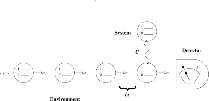
FIG. 1.: This is a schematic diagram of the type of model used in this paper. The system is a single two-level system, or q-bit. It interacts briefly with a series of environment q-bits which pass by with average time intervals of $\delta t$, and the environment bits are subsequently measured.

FIG. 2.: Here is a particular physical system of which the model of this paper is an idealization. The system is an electromagnetic field mode in a cavity with a partially-silvered mirror. There is on average less than a single photon in the mode at a time, so only the lowest two occupation levels contribute significantly to the dynamics. The external electromagnetic field is described in terms of incoming and outgoing wave packets of width $\delta t$, each of which reflects on the outside of the partially-silvered mirror. The incoming packets are all in the vacuum state, but upon reflection they may absorb a photon emitted from the cavity.

FIG. 3.: These two figures show a variety of quantum jump trajectories for different initial states, plotting the squared amplitude $|\beta|^{2}$ for the system to be in state ${|1\rangle}$ versus the time. Figure a) assumes an interaction ${\hat{U}}_{\rm CNOT}$ with the environment, while b) assumes ${\hat{U}}_{\rm SWAP}$. In both cases, $|\beta|^{2}$ decays towards zero. Some trajectories just decay smoothly to 0, while others undergo a jump. In figure a) this jump is to 1, while in b) they jump to 0, as in spontaneous emission. Note that the decays of $|\beta|^{2}$ is not a simple exponential, due to the nonlinearity of the trajectory equations. As $|\beta|^{2}\rightarrow 0$, however, it approaches an exponential.

FIG. 4.: This figure plots $|\beta|^{2}$ against time for the diffusive equation (140), with several different initial states and realizations of the stochastic term. We see that when the trajectories approach 0 or 1 they tend to remain there, while in between they diffuse freely.

REFERENCES

- [1] H.J. Carmichael, An Open Systems Approach to Quantum Optics, (Springer, Berlin, 1993).
- [2] J. Dalibard, Y. Castin and K. Mølmer, Phys. Rev. Lett. 68, 580 (1992).
- [3] R. Dum, P. Zoller and H. Ritsch, Phys. Rev. A 45, 4879 (1992).
- [4] C.W. Gardiner, A.S. Parkins and P. Zoller, Phys. Rev. A 46, 4363 (1992).
- [5] N. Gisin, Phys. Rev. Lett. 52, 1657 (1984); Helv. Phys. Acta. 62, 363 (1989).
- [6] L. Diósi, J. Phys. A 21, 2885 (1988); Phys. Lett. 129A, 419 (1988); Phys. Lett. 132A, 233 (1988).
- [7] N. Gisin and I.C. Percival, J. Phys. A 25, 5677 (1992); J. Phys. A 26, 2233, 2245 (1993).
- [8] R. Schack, T.A. Brun and I.C. Percival, J. Phys. A 28, 5401 (1995).
- [9] H.D. Zeh, Found. Phys. Lett. 12, 197 (1999).
- [10] P. Pearle, Phys. Rev. D 13, 857 (1976); Int. J. Theor. Phys. 18, 489 (1979).
- [11] G.C. Ghirardi, A. Rimini and T. Weber, Phys. Rev. D 34, 470 (1986).
- [12] I.C. Percival, Proc. Roy. Soc. A 447, 189 (1994); ibid. 451, 503 (1995).
- [13] R. Penrose, in Bangalore 1994, Non-accelerator particle physics, 416, edited by R. Cowsik, (World Scientific, River Edge, N.J., 1995).
- [14] M.A. Nielsen and I.L. Chuang, Quantum Computation and Quantum Information (Cambridge University Press, Cambridge, 2000).
- [15] A. Peres, Quantum Theory: Concepts and Methods, (Kluwer, Dordrecht, 1993).
- [16] L. Vaidman, in Advances in quantum phenomena, 357, edited by E.G. Beltrametti and J.-M. Levy-Leblond, (Plenum Press, 1995).
- [17] W.H. Zurek, Phys. Rev. D 24, 1516 (1981); Phys. Rev. D 26, 1862 (1982); Physics Today 44, 36 (1991).
- [18] E. Joos and H.D. Zeh, Z. Phys. B 59, 229 (1985).
- [19] G. Lindblad, Commun. Math. Phys. 48, 119 (1976).
- [20] B. Misra and E.C.G. Sudarshan, J. Math. Phys. 18, 756 (1977).
- [21] H.M. Wiseman and G.J. Milburn, Phys. Rev. A 47, 1652 (1993).
- [22] A.N. Soklakov and R. Schack, J. Mod. Optics 47, 2265 (2000).
- [23] E. Schrödinger, Naturwissenschaften 23, 807, 823, 844 (1935).
- [24] J.S. Bell, Physics 1, 195 (1964).
- [25] D. Bohm, Phys. Rev. 85, 166 (1952).
- [26] I.C. Percival and W.T. Strunz, Proc. Roy. Soc. Lond. A453, 431 (1997); W.L. Power and I.C. Percival, ibid. A456, 955 (2000).
- [27] S.L. Adler and T.A. Brun, submitted to J. Phys. A, quant-ph/0103037.
- [28] R.B. Griffiths, J. Stat. Phys. 36, 219 (1984); Phys. Rev. A 54, 2759 (1996); ibid. 57, 1604 (1998).
- [29] R. Omnès, The Interpretation of Quantum Mechanics, (Princeton University Press, Princeton, 1994); Understanding Quantum Mechanics, (Princeton University Press, Princeton, 1999).
- [30] M. Gell-Mann and J.B. Hartle, in Complexity, Entropy, and the Physics of Information, SFI Studies in the Science of Complexity v. VIII, edited by W. Zurek, 425 (Addison-Wesley, Reading, 1990); in Proceedings of the Third International Symposium on the Foundations of Quantum Mechanics in the Light of New Technology, edited by S. Kobayashi, H. Ezawa, Y. Murayama, and S. Nomura, 321 (Physical Society of Japan, Tokyo, 1990); in Proceedings of the 25th International Conference on High Energy Physics, Singapore, 2–8 August 1990, edited by K.K. Phua and Y. Yamaguchi, (World Scientific, Singapore, 1990).
- [31] L. Diósi, N. Gisin, J.J. Halliwell and I.C. Percival, Phys. Rev. Lett. 21, 203 (1995).
- [32] T.A. Brun, Phys. Rev. Lett. 78, 1833 (1997).
- [33] T.A. Brun, Phys. Rev. A 61, 042107 (2000).