Inverse Quantum Zeno Effect in Quantum Oscillations

Abstract

It is shown that inverse quantum Zeno effect (IZE) may exist in a three-level system with Rabi oscillations between discrete atomic states. The experiment to observe IZE in such a system is proposed.

1 Introduction

It is known that frequently repeated discrete quantum measurements can hinder quantum transitions. This phenomenon is known as quantum Zeno effect (QZE) [1, 2]. This effect was found experimentally in systems with forced Rabi oscillations between discrete atomic levels [3] and in spontaneously decaying systems [4]. It was shown also that there are regimes when repeated discrete measurements can accelerate spontaneous decay [5, 6, 7], and this phenomenon was found experimentally as well [4]. This effect is known as anti Zeno effect or inverse Zeno effect (IZE).

In the present paper the definitions for QZE and IZE are admitted in agreement with that introduced by P. Facchi and S. Pascazio [8] with one modification. Let the initial pure state of a system with Hamiltonian $H$ be $\rho_{0}$ and the survival probability be $P(t)={\rm Tr}[\rho_{0}\rho(t)]$. Consider the evolution of system under the effect of an additional interaction, so that the total Hamiltonian reads

$$H_{K}=H+H_{\rm meas}(K),$$

where $K$ is a set of parameters and $H_{\rm meas}(K=0)=0$. $H$ is a full Hamiltonian of the system containing interaction terms, and $H_{\rm meas}(K)$ should be considered as an additional Hamiltonian performing the measurement. The term $H_{\rm meas}(K)$ may describe a chain of ideal discrete quantum measurements that are represented by reductions (collapses) of state of the system as a special case of interaction. The system displays QZE if there exist an interval $I^{(K)}=[t_{1}^{(K)},t_{2}^{(K)}]$ such that

$$P^{(K)}(t)>P(t),\quad\forall t\in I^{(K)},$$ (1)

and the system displays IZE if there exist an interval $I^{(K)}$ such that

$$P^{(K)}(t)<P(t),\quad\forall t\in I^{(K)}.$$ (2)

Here $P^{(K)}(t)$ and $P(t)$ are the survival probabilities under the action of $H_{K}$ and $H$, respectively, and it is required

$$t^{(K)}_{2}\leq T_{P},$$ (3)

where $T_{P}$ is the Poincaré time. The modification of this definitions is the following. In the addition to the definitions Eqs. (1,2,3) it is required:

• The Hamiltonian of measurement $H_{\rm meas}(K)$ is to be time-independent or periodical with the period less then the Poincaré time of the system.

The meaning of condition (i) is the following. Johann von Neumann proved the following proposition [9, Chapter V.2]. Using a sequence of frequently repeated measurements represented by time-dependent projections it is possible to force the quantum system pass through arbitrary definite sequence of states. Particularly, it is possible to satisfy the conditions of Eqs. (2,3) which define IZE. But such a situation does not appear to be IZE, rather it is a dynamical version of usual quantum Zeno effect (dynamical quantum Zeno effect, DQZE). Though DQZE is considered as “anti-Zeno paradox” some times [10], such interpretation seems to be misleading. The condition (i) is intended to avoid such misunderstands.

It was pointed out many times (see [7] and references herein) that both QZE and IZE can be obtained for a genuinely unstable system, whose Poincaré time is infinite. On the other hand, the possibility of IZE for an oscillating quantum mechanical system, whose Poincaré time is finite, was not reported up to now. Actually, only QZE is possible in two-level quantum mechanical oscillating systems. But it is not generally valid in multilevel systems with the number of levels more than two. In the present paper a three-level oscillating system with finite Poincaré time exhibiting IZE is constructed.

2 Interaction picture for evolution interrupted by measurements

Before discussing of the main subject we introduce the interaction picture formalisms for the problem of quantum evolution interrupted by discrete measurements. Let $H=H_{0}+V$ be a Hamiltonian of a system $S$ and $\rho(t)$ be the density operator of this system. Let $\{P_{i}\}$, $P_{i}^{2}=P_{i}$, $\sum_{i}P_{i}=1$ be a complete set of projection operators. This set of projectors represents an instantaneous reduction of system state following an ideal quantum measurement. The change of state during the measurement is

$$\rho^{\prime}=\sum_{i}P_{i}\rho P_{i}\equiv\hat{R}\rho,$$ (4)

where $\rho$ is the state before the measurement and $\rho^{\prime}$ is the state after the measurement. Let $D(t)\,dt$ be the probability of carrying out the measurement on the system during time interval $(t,t+dt)$. Then, it is easy to prove that the state of system is governed by the Lindblad equation

$$\frac{d\rho}{dt}=-\frac{i}{\hbar}[H_{0}+V,\rho]-\frac{1}{2}D(t)\sum_{i}[P_{i},[P_{i},\rho]].$$ (5)

Let $\rho_{I}(t)$ and $V_{I}(t)$ be the state and the Hamiltonian of the system in interaction picture:

$$\rho_{I}(t) = \exp\left(\frac{i}{\hbar}H_{0}t\right)\rho(t)\exp\left(-\frac{i}{\hbar}H_{0}t\right)$$ (6)

$$V_{I}(t) = \exp\left(\frac{i}{\hbar}H_{0}t\right)V\exp\left(-\frac{i}{\hbar}H_{0}t\right).$$ (7)

Further, let

$$[P_{i},H_{0}]=0\quad\forall i.$$ (8)

By direct substitution of Eqs. (6,7) in Eq. (5) and accounting for Eq. (8) it is not hard to prove that

$$\frac{d\rho_{I}}{dt}=-\frac{i}{\hbar}[V_{I},\rho_{I}]-\frac{1}{2}D(t)\sum_{i}[P_{i},[P_{i},\rho_{I}]].$$ (9)

Equation (9) is a generalization of Lindblad equation (5) for the interaction picture of evolution.

Let consider the evolution of the system during the time interval $(0,t)$. Let $t_{0},t_{1},\dots,t_{n}$ be moments of time such that $t_{0}=0<t_{1}<\dots<t_{n-1}<t_{n}=t$. Then Eq. (5) and Eq. (9) are also valid for the singular distribution $D(t)$:

$$D(t)=\sum_{k=0}^{n}\delta(t-t_{k}).$$

where $\delta()$ is the Dirac’s delta-function. This special distribution $D(t)$ describes the sequence of measurements at the definite moments of time $t_{0},t_{1},\dots,t_{n}$. It is not hard to understand that the solution of Eq. (9) for this special $D(t)$ may be written as

$$\rho_{I}(t)=\hat{R}\hat{U}_{I}(t_{n},t_{n-1})\cdots\hat{R}\hat{U}_{I}(t_{1},t_{0})\hat{R}\rho(t_{0}),$$ (10)

where the superoperator of reduction $\hat{R}$ is defined by Eq. (4) and the superoperator of evolution

$$\hat{U}_{I}(t^{\prime\prime},t^{\prime})\rho=U_{I}(t^{\prime\prime},t^{\prime})\rho U_{I}^{+}(t^{\prime\prime},t^{\prime})$$ (11)

is defined by the solution of Shrödinger equation in the interaction picture without measurements:

$$\frac{d\rho_{I}}{dt}=-\frac{i}{\hbar}[V_{I},\rho].$$

If the system was prepared in the pure eigenstate $|\Psi_{0}\rangle$ of Hamiltonian $H_{0}$ at the initial moment of time $t_{0}=0$, then it is easily shown that the survival probability $P(t)$ would be

$$P(t)=\langle\Psi_{0}|\rho_{I}(t)|\Psi_{0}\rangle,$$ (12)

where $\rho_{I}(t)$ is defined by Eq. (10).

3 Model system

Let consider three-level atom with free Hamiltonian $H_{0}$ and eigenstates $|0\rangle,|1\rangle,|2\rangle$:

$$H_{0}|j\rangle = \hbar\omega_{j}|j\rangle,\quad j=0,1,2$$ (13)

$$\omega_{ij} = \omega_{i}-\omega_{j},\quad i\neq j.$$

Let the initial state of the atom be $|\Psi_{0}\rangle=|0\rangle.$ The atom interacts with the classical electric field consisting of two components being in resonance with the transitions $\omega_{10}$ and $\omega_{21}$, respectively:

$${\rm\bf E}(t)={\rm\bf E}_{10}e^{i\omega_{10}t}+{\rm\bf E}_{10}^{*}e^{-i\omega_{10}t}+{\rm\bf E}_{21}e^{i\omega_{21}t}+{\rm\bf E}_{21}^{*}e^{-i\omega_{21}t},$$ (14)

where ${\rm\bf E}_{10}$ and ${\rm\bf E}_{21}$ are arbitrary complex amplitudes of fields. The interaction of electric field with the atom is

$$V=-{\rm\bf D}{\rm\bf E},$$ (15)

where ${\rm\bf D}$ is the operator of dipole moment of the atom. The following relations are admitted to be valid:

$$|\omega_{ij}| \gg |V_{mn}|\quad\forall i,j,m,n;$$ (16)

$$|\omega_{ij}-\omega_{kl}| \gg |V_{mn}|\quad\forall i,j,k,l:\{i,j\}\neq\{k,l\},\quad\forall m,n,$$ (17)

where $V_{mn}=\langle m|V|n\rangle$.

Let consider the evolution of atom during time interval $(0,t)$. Suppose that the measurement $\hat{R}$ is carried out on the atom at the moments $t_{0},t_{1},\dots t_{n}$ where $t_{k}=k\Delta t,\Delta t=t/n$, $n=1,2,3,\dots$ . The measurement $\hat{R}$ is intended to determine whether the atom is on the level $|2\rangle$ or not. Therefore, the superoperator $\hat{R}$ reads

$$\hat{R}\rho=P_{01}\rho P_{01}+P_{2}\rho P_{2},$$ (18)

where

$$P_{01}={\rm diag}(1,1,0),\quad P_{2}={\rm diag}(0,0,1).$$ (19)

Let find the probability that the atom is at the state $|0\rangle$ at time $t$. This probability is the survival probability $P(t)$ Eq. (12) for $|\Psi_{0}\rangle=|0\rangle$. To determine $\rho_{I}(t)$ one can use Eq. (10). Further, $\hat{R}$ in Eq. (10) is already known from Eq. (18). Consequently, $\hat{U}_{I}(t^{\prime\prime},t^{\prime})$ is to be calculated.

Let $a(t)$ be a three-dimensional complex vector, $a=[a_{0},a_{1},a_{2}]$. Consider the equation

$$\frac{da(t)}{dt}=-\frac{i}{\hbar}V_{I}(t)a(t)$$ (20)

with the initial conditions defined for the time $t^{\prime}$: $a(t^{\prime})=[a^{0}_{0},a^{0}_{1},a^{0}_{2}]$. In Eq. (20) $V_{I}(t)$ is the interaction picture Hamiltonian for the free Hamiltonian Eq. (13) and the interaction Eq. (15). The solution of Eq. (20) for the time $t^{\prime\prime}$ may be written as

$$a(t^{\prime\prime})=U_{I}(t^{\prime\prime},t^{\prime})a(t^{\prime}),$$ (21)

where $U_{I}(t^{\prime\prime},t^{\prime})$ is the evolution operator that is needed for calculation of $\hat{U}_{I}(t^{\prime\prime},t^{\prime})$ by Eq. (11). Using Eqs. (14,15) and the rotating wave approximation (which is right under the conditions (16,17)), one can rewrite Eq. (20) as

$$\frac{d}{dt}\left(\begin{array}[]{ccc}a_{0}\\ a_{1}\\ a_{2}\end{array}\right)=-i\left(\begin{array}[]{ccc}0&\Omega_{01}e^{i\varphi_{01}}&0\\ \Omega_{01}e^{-i\varphi_{01}}&0&\Omega_{12}e^{i\varphi_{12}}\\ 0&\Omega_{12}e^{-i\varphi_{12}}&0\\ \end{array}\right)\left(\begin{array}[]{ccc}a_{0}\\ a_{1}\\ a_{2}\end{array}\right),$$ (22)

where the notations

$$\Omega_{01}e^{i\varphi_{01}}=-\langle 0|{\rm\bf D}|1\rangle{\rm\bf E}_{1}/\hbar,\quad\Omega_{12}e^{i\varphi_{12}}=-\langle 1|{\rm\bf D}|2\rangle{\rm\bf E}_{2}/\hbar,$$

were introduced. The values $\Omega_{01}$ and $\Omega_{12}$ are considered to be positive real numbers. The evolution operator $U_{I}(t^{\prime\prime},t^{\prime})$ may be obtained by solution Eq. (22) and comparison the results with Eq. (21):

$$\begin{array}[]{l}\displaystyle U_{I}(t^{\prime\prime},t^{\prime})=\\ \\ \left(\begin{array}[]{ccc}\displaystyle\frac{\Omega_{12}^{2}+\Omega_{01}^{2}\cos\alpha}{\Omega^{2}}&\displaystyle-i\frac{\Omega_{01}}{\Omega}e^{i\varphi_{01}}\sin\alpha&\displaystyle-\frac{\Omega_{01}\Omega_{12}}{\Omega^{2}}e^{i(\varphi_{01}+\varphi_{12})}(1-\cos\alpha)\\ \displaystyle-i\frac{\Omega_{01}}{\Omega}e^{-i\varphi_{01}}\sin\alpha&\displaystyle\cos\alpha&\displaystyle-i\frac{\Omega_{12}}{\Omega}e^{i\varphi_{12}}\sin\alpha\\ \displaystyle-\frac{\Omega_{01}\Omega_{12}}{\Omega^{2}}e^{-i(\varphi_{01}+\varphi_{12})}(1-\cos\alpha)&\displaystyle-i\frac{\Omega_{12}}{\Omega}e^{-i\varphi_{12}}\sin\alpha&\displaystyle\frac{\Omega_{01}^{2}+\Omega_{12}^{2}\cos\alpha}{\Omega^{2}}\end{array}\right),\end{array}$$ (23)

where

$$\Omega=\sqrt{\Omega_{01}^{2}+\Omega_{02}^{2}}\,;\quad\alpha=\Omega(t^{\prime\prime}-t^{\prime}).$$

Now both values, $\hat{R}$ (from Eqs. (18,19)) and $\hat{U}_{I}(t^{\prime\prime},t^{\prime})$ (from Eqs. (11,23)), are known, and the survival probability for state $|0\rangle$ may be calculated by Eqs. (10,12).

4 Results of calculations and discussion

Firstly, let us discuss the mechanisms of IZE in this system qualitatively. For the beginning suppose that the measurements are absent at all. Since the initial state of system $|\Psi_{0}\rangle=|0\rangle$ was pure at the moment $t_{0}=0$ so it will be pure in future, and the evolution will be governed only by the operator $U_{I}(t^{\prime\prime},t^{\prime})$: $|\Psi_{I}(t)\rangle=U_{I}(t,0)|0\rangle.$ Suppose $\Omega_{12}=0$. It is seen from Eq. (23) that the evolution of the atom is reduced to the usual Rabi oscillations:

$$a_{0}(t)=\cos\Omega_{01}t;\quad a_{1}(t)=-i\sin\Omega_{01}t;\quad a_{2}(t)=0.$$

In the converse case, $\Omega_{12}\gg\Omega_{01}$, Eq. (23) shows that the initial state is ”frozen”:

$$\forall t:\quad a_{0}(t)\approx 1;\quad a_{1}(t)\approx 0;\quad a_{2}(t)\approx 0.$$

Generally speaking, the transition between states $|1\rangle$ and $|2\rangle$ hinders the transition between states $|0\rangle$ and $|1\rangle$. This is well-known phenomenon [11, 12, 8] which is considered as a Zeno-like effect. However, if the transition $|1\rangle\to|2\rangle$ itself is continuously observed by frequent measurements represented by Eq. (18), then the transition $|1\rangle\to|2\rangle$ will be ”frozen” by usual QZE, and the mentioned above Zeno-like effect will be hindered by this usual Zeno effect. Rabi transition $|0\rangle\to|1\rangle$ becomes possible followed by the state $|0\rangle$ ”defreezes”. And this is IZE.

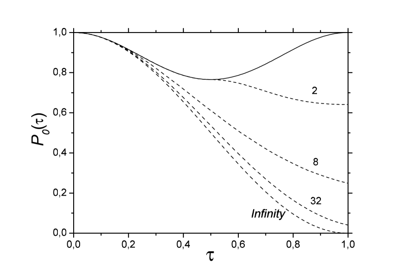
To represent the detailed calculations, $\Omega_{12}=\Omega_{01}\sqrt{15}$ is chosen. Hence $\Omega=4\Omega_{01}$ and it is seen from Eq. (23) that the Poincaré time of the system is

$$T_{P}=2\pi/\Omega=\pi/(2\Omega_{01}).$$ (24)

The solid line on Fig. 1 represents the “free” evolution of the atom during one Poincaré time: both resonant components of electric field is switched on, but measurements is switched off. Dashed lines represent the evolution with different numbers of measurements during the interval $t\in(0,T_{P})$; the number near the line is the number $n$ as in Eq. (10). It is seen from Fig. 1 that IZE takes place in the exact accordance with the definition of IZE by Eqs. (2,3) and condition (i). Moreover, the evolution of the atom tends to the free Rabi transition between levels $|0\rangle$ and $|1\rangle$ with frequency $2\Omega_{01}$ as $n\to\infty$, as one should expect.

The model three-level system with double Rabi transition and measurements described in the present paper may be realized in the experiment similar to Itano and collaborators QZE-experiment with simple Rabi transition [3]. The levels $|0\rangle,|1\rangle,|2\rangle$ of the atom may correspond to fine or hyperfine structure. Rabi transitions between these levels may be forced by ultra high frequency or radio frequency fields. In the addition the forth level $|3\rangle$ should be involved such that it should be higher than level $|2\rangle$ and the transition $|3\rangle\to|2\rangle$ should be a no-forbidden optical transition. The state $|3\rangle$ is to decay onto the state $|2\rangle$ much faster than all Rabi transitions involved to the experiment. A short $\pi$-pulse of laser tuned to the resonance with the transition $|3\rangle\to|2\rangle$ will simulate the measurement $\hat{R}$, Eq. (18). The probability of finding the atom in the state $|0\rangle$ at the end of evolution may be measured by the usual way [3].

The author acknowledges the fruitful discussions with P. Facchi, M. B. Mensky, and S .Pascazio and is grateful to V. A. Arefjev for the help in preparation of the paper.

Figure 1: Inverse Zeno effect in a three-level atom with double Rabi transition. $\tau=t/T_{P}$, where Poincaré time $T_{P}$ is defined by Eq. (24); $P_{0}(\tau)$ is the probability to find the atom in the initial state $|0\rangle$. Solid line reperesents the evolution of atom without measurements, dashed lines represent the evolution of atom with different number of measurements during the interval $\tau\in(0,1)$.

References

- [1] B. Misra and E. C. G. Sudarshan, J. Math. Phys. 18, 756 (1977).
- [2] C. B. Chiu, E. C. G. Sudarshan, and B. Misra, Phys. Rev. D 16, 520 (1977).
- [3] W. M. Itano, D. J. Heinzen, J. J. Bollinger, and D. J. Wineland, Phys. Rev. A 41, 2295 (1990).
- [4] M. C. Fisher, B. Gutiérrez-Medina, and M. G. Raizen, Observation of Quantum Zeno and Anti-Zeno effects in an unstable system, quant-ph/0104035, 2001.
- [5] G. Bernardini, L. Maiani, and M. Testa, Phys. Rev. Lett. 71, 2687 (1993).
- [6] P. Facchi and S. Pascazio, Physics Letters. A 241, 139 (1998).
- [7] P. Facchi, H. Nakazato, and S. Pascazio, Phys. Rev. Lett. 86, 2699 (2001).
- [8] P. Facchi and S. Pascazio, Quantum Zeno and inverse Zeno effects, Review, 2001.
- [9] J. von Neumann, Mathematische Grundlagen der Quantenmechanik (Springer, Berlin, 1932).
- [10] A. P. Balachandran and S. M. Roy, Continuous time-dependent measurements: quantum anti-Zeno paradox with applications, quant-ph/0102019, 2001.
- [11] A. Peres, Am. J. Phys 48, 931 (1980).
- [12] K. Kraus, Found. Phys. 11, 547 (1981).