Beyond the Fokker-Planck equation: Stochastic Simulation of Complete Wigner representation for the Optical Parametric Oscillator

Abstract

We demonstrate a method which allows the stochastic modelling of quantum systems for which the generalised Fokker-Planck equation in the phase space contains derivatives of higher than second order. This generalises quantum stochastics far beyond the quantum-optical paradigm of three and four-wave mixing problems to which these techniques have so far only been applicable. To verify our method, we model a full Wigner representation for the optical parametric oscillator, a system where the correct results are well known and can be obtained by other methods.

I Introduction

Coherent-state, or phase-space, path integrals [1] are so far the only variety of path integrals that can be evaluated numerically for real time problems. For interactions which are no more than quadratic in creation or annihilation operators, the measure over the paths can be described in terms of stochastic differential equations (SDEs, Langevin equations) for the paths [2, 3]. Unlike, e.g., the Feynman path integral, such real-time phase-space path integrals are characterised by a constructively defined positive measure, and can be calculated by simulating the corresponding Langevin equations. These techniques have been most successfully used in quantum optics [2], but have also been applied to the quantum dynamics of condensed bosonic atoms [4]. Mathematically, however, the existence of an SDE for the paths is restricted to problems were the equation for the corresponding pseudo-probability distribution is a genuine Fokker-Planck equation (this is the content of Pawula’s theorem [5]). This imposes the above restriction on the interaction Hamiltonian and thus confines the class of problems for which the measure of the path integral may be characterised in terms of an SDE to three and four-wave mixing problems. (The two-body collisional interaction of bosons has the formal structure of four wave mixing.)

There exist, however, a wide variety of problems where the generalised Fokker-Planck equation is of third or higher order and hence Langevin equations may not be derived. As an example, a description of nonlinear quantum optical processes in terms of the Wigner distribution results in generalised Fokker-Planck equations with third-order derivatives [3]. A common procedure is to truncate the Wigner equation at second order, which is equivalent to using the semiclassical theory of stochastic electrodynamics [6]. This procedure necessarily discards the deeper quantum aspects of the problem and gives answers at odds with quantum mechanics for several systems [7]. There are also situations where even a P-representation Fokker-Planck equation must also be written in generalised form [8], and more are likely to be investigated in the future. It is therefore of considerable interest to generalise methods allowing for a constructive characterisation of the measure of the phase-space path integral beyond the very restrictive quantum-optical paradigm.

Pawula’s theorem would at first sight seem to forbid this generalisation. However, on closer inspection we see that the restrictions imposed can be evaded by discretising time. Full technical details are presented elsewhere [9]; the aim of this letter is to demonstrate the feasibility of this generalisation, using as a demonstrative example the Wigner representation for the optical parametric oscillator (OPO). We chose this system because it is well known and the results can be obtained by other methods. We derive a system of stochastic difference equations in a doubled phase-space, which is related to the Wigner representation in the same way as the well-known positive-P equations [10] are related to the P-representation. By analogy, we shall call this representation the positive-W representation. We show that this representation gives the correct results for quadrature relaxation, whereas the truncated Wigner representation makes noticeably different predictions.

It should be stressed that no continuous time limit exists for the positive-W equations. Unlike the Wiener process, where sampling noise is independent of the time step for a given sample size, here sampling noise diverges in the continuous time limit. This is how Pawula’s theorem is enforced. In practice, however, one is interested in the sampling noise vs time step not for a given sample size, but for a given computational time. From this perspective, the difference we find is much less dramatic. Although, as the time step is decreased, the computational time grows at a faster rate than for conventional stochastic integration, this dependence remains polynomial so that the problem stays in the same class of computational complexity.

II Positive-W representation

Degenerate optical parametric oscillation is an optical process in which a nonlinear medium inside an optical cavity is pumped with light at one frequency and emits light at half that frequency. The free, damping and pumping Hamiltonians for this system may be written in their usual forms [11] while we choose the nonlinear coupling constant between the light modes, $\kappa$, to be real so that the interaction Hamiltonian is

$$H_{{\rm int}}=\frac{i\hbar\kappa}{2}\left[\hat{a}^{{\dagger}\;2}\hat{b}-\hat{a}^{2}\hat{b}^{{\dagger}}\right].$$ (1)

The annihilation (creation) operators $\hat{a}\;(\hat{a}^{{\dagger}})$ and $\hat{b}\;(\hat{b}^{{\dagger}})$ annihilate (create) photons at the lower and higher frequencies respectively. Proceeding via the usual methods, we can map the Hamiltonian onto differential equations for the Wigner and positive-P distributions [2]. The positive-P representation gives a Fokker-Planck equation and can thus be mapped straightforwardly onto a set of coupled SDEs using Itô rules. The equation of motion for the Wigner distribution, however, has third-order derivatives and thus has no mapping onto stochastic differential equations.

The positive-P representation can alternatively be derived [9] by postulating a mapping of time-normal ($T_{N}$) averages [12] of the Heisenberg quantum-field operators, $\hat{\sl a}^{{\dagger}}(t),\hat{\sl b}^{{\dagger}}(t),\hat{\sl a}(t)$, $\hat{\sl b}(t)$, onto classical averages. For example,

$$\left\langle T_{N}\left\{\hat{\sl a}^{{\dagger}}(t)\hat{\sl b}^{{\dagger}}(t^{\prime})\hat{\sl a}(t^{\prime\prime})\hat{\sl b}(t^{\prime\prime\prime})\right\}\right\rangle \equiv \left\langle T_{-}\left\{\hat{\sl a}^{{\dagger}}(t)\hat{\sl b}^{{\dagger}}(t^{\prime})\right\}T_{+}\left\{\hat{\sl a}(t^{\prime\prime})\hat{\sl b}(t^{\prime\prime\prime})\right\}\right\rangle$$ (2)

$$= \overline{\hskip 0.43057pt{a}^{{\dagger}}(t){b}^{{\dagger}}(t^{\prime}){a}(t^{\prime\prime}){b}(t^{\prime\prime\prime})\hskip 0.43057pt}\ .$$ (3)

The upper bar on the RHS of this relation denotes averaging over the statistics of the four stochastic c-number fields, ${a}^{{\dagger}}(t),{b}^{{\dagger}}(t),{a}(t),{b}(t)$ (i.e. phase-space path integration). The essence of the positive-P representation is in defining these statistics constructively. The Heisenberg equations of motion are mapped onto the SDE’s for the fields, while the averaging over the initial state of the quantum field (denoted as $\left\langle\cdots\right\rangle$) is mapped onto the distribution over the initial conditions.

The $T_{N}$ ordering emerges when we generalise the normal ordering of free-field operators to the Heisenberg operators. Generalising the symmetric, or Wigner, ordering of free-field operators results in a time-Wigner ($T_{W}$) ordering of the Heisenberg field operators [9]. Under $T_{N}$, the “most recent” creation (annihilation) operator becomes the leftmost (rightmost) in the product. The $T_{W}$-ordering acts in a similar way except that it is symmetrised with respect to the creation and annihilation operators:

$$T_{W}\left\{\hat{\sl x}(t)\hat{\sl y}(t^{\prime})\cdots\hat{\sl z}(t^{\prime\prime})\right\} = \frac{1}{2}\left[T_{W}\left\{\hat{\sl y}(t^{\prime})\cdots\hat{\sl z}(t^{\prime\prime})\right\}\hat{\sl x}(t)\right.$$ (5)

$$+\,\left.\hat{\sl x}(t)T_{W}\left\{\hat{\sl y}(t^{\prime})\cdots\hat{\sl z}(t^{\prime\prime})\right\}\right].$$

Here, $\hat{\sl x},\hat{\sl y},\cdots,\hat{\sl z}$ stand for field operators (i.e. $\hat{\sl a}$ or $\hat{\sl a}^{{\dagger}}$), and $t$ should exceed all other time arguments in the product so that $t>t^{\prime},\cdots,t^{\prime\prime}$. Equation (5) is a recurrence relation which defines $T_{W}$ for the case of different time arguments. The full definition may be found in [9].

Following the example of the positive-P mapping (2), we postulate a positive-W mapping relating $T_{W}$-ordered operator averages to classical averages of four stochastic c-number fields, $\alpha(t),\alpha^{{\dagger}}(t),\beta(t),\beta^{{\dagger}}(t)$, so that, e.g.,

$$\left\langle T_{W}\left\{\hat{\sl a}^{{\dagger}}(t)\hat{\sl b}^{{\dagger}}(t^{\prime})\hat{\sl a}(t^{\prime\prime})\hat{\sl b}(t^{\prime\prime\prime})\right\}\right\rangle=\overline{\hskip 0.43057pt{\alpha}^{{\dagger}}(t){\beta}^{{\dagger}}(t^{\prime}){\alpha}(t^{\prime\prime}){\beta}(t^{\prime\prime\prime})\hskip 0.43057pt}.$$ (6)

We emphasise that this mapping is distinct from that of Eq. (2) by changing the notation of the c-number fields. In full detail, the quantum-field-theoretical (QFT) techniques which we used in order to characterise the mapping (6) constructively are described elsewhere [9, 13]. For the purposes of this letter, we note that these are a straightforward adaptation of similar QFT techniques described in Refs. [14, 15]. In [14], Matsubara-style quantum dynamics were mapped onto an imaginary-time SDE; in [15], Feynman diagram techniques were mapped onto a real-time SDE. Here, we consider dynamics on the Schwinger-Keldysh C-contour [16]. To include the Wigner representation, one needs a generalisation of Wick’s theorem to the case of symmetric ordering. This generalisation is quite straightforward and results in a Keldysh-style diagram series for the $T_{W}$-ordered averages. As in [14, 15], propagators in this diagram series are then expressed by the retarded Green’s function of the free Schrödinger equation, and the whole series is restructured so as to make this Green’s function a propagator in a new series. This yields a Wyld-type series [17], also termed causal series [13]. By applying multiple Hubbard-Stratonovich transformations [18], we eventually arrive at a classical stochastic problem for which this series is a solution. This final step of the derivation is of independent interest and is discussed in more detail below.

In the strict mathematical sense, this derivation fails: no continuous-time process exists satisfying Eq. (6). The way around this problem is to allow the mapping (6) to hold only approximately, and consider stochastic processes in discretised time. We then find the following set of stochastic difference equations, (dropping the $t$-dependence for notational simplicity)

$$\Delta\alpha = \left(-\gamma_{1}\alpha+\kappa\alpha^{{\dagger}}\beta\right)\Delta t+\sqrt{\gamma_{1}}\eta_{1}\Delta t^{1/2}+\sigma_{1}\Delta t^{1/3},$$ (7)

$$\Delta\alpha^{{\dagger}} = \left(-\gamma_{1}\alpha^{{\dagger}}+\kappa\alpha\beta^{{\dagger}}\right)\Delta t+\sqrt{\gamma_{1}}\eta_{1}^{\ast}\Delta t^{1/2}+\sigma_{1}^{{\dagger}}\Delta t^{1/3},$$ (8)

$$\Delta\beta = \left(\epsilon-\gamma_{2}\beta-\frac{\kappa}{2}\alpha^{2}\right)\Delta t+\sqrt{\gamma_{2}}\eta_{2}\Delta t^{1/2}+\sigma_{2}\Delta t^{1/3},$$ (9)

$$\Delta\beta^{{\dagger}} = \left(\epsilon^{\ast}-\gamma_{2}\beta^{{\dagger}}-\frac{\kappa}{2}\alpha^{{\dagger}\;2}\right)\Delta t+\sqrt{\gamma_{2}}\eta_{2}^{\ast}\Delta t^{1/2}+\sigma_{2}^{{\dagger}}\Delta t^{1/3},$$ (10)

where $\Delta t$ is the step of time discretisation, $\Delta\alpha(t)=\alpha(t+\Delta t)-\alpha(t)$ (likewise for the other field variables) and $\eta_{1,2}(t)$ are independent complex standardised Gaussian noises such that

$$\overline{\hskip 0.43057pt\eta_{1}(t)\hskip 0.43057pt}=\overline{\hskip 0.43057pt\eta_{2}(t)\hskip 0.43057pt}=0,\ \ \overline{\hskip 0.43057pt\eta_{1}(t)\eta_{1}(t^{\prime})\hskip 0.43057pt}=\overline{\hskip 0.43057pt\eta_{2}(t)\eta_{2}(t^{\prime})\hskip 0.43057pt}=0,\ \ \overline{\hskip 0.43057pt\eta_{1}(t)\eta_{1}^{*}(t^{\prime})\hskip 0.43057pt}=\overline{\hskip 0.43057pt\eta_{2}(t)\eta_{2}^{*}(t^{\prime})\hskip 0.43057pt}=\delta_{tt^{\prime}}.$$ (11)

It should be noted that the $\eta$’s are $\delta_{tt^{\prime}}$ (Kronecker) correlated, not $\delta(t-t^{\prime})$ (Dirac) correlated and that we have explicitly taken care of the proper powers of $\Delta t$. The $\gamma_{j},\ j=1,2$, are the cavity loss rates at each frequency and $\epsilon$ represents the classical pump. For the $\sigma$’s we have

$$\sigma_{1}=q\xi_{2}+s\,\xi_{1}^{{\dagger}*}\sqrt{p^{{\dagger}}\xi_{2}^{*}}\,,\ \ \sigma_{1}^{{\dagger}}=q^{{\dagger}}\xi_{2}^{{\dagger}}+s^{{\dagger}}\,\xi_{1}^{*}\sqrt{p\xi_{2}^{{\dagger}*}}\,,\ \ \sigma_{2}=r\xi_{1}\sqrt{p\xi_{2}^{{\dagger}*}}\,,\ \ \sigma_{2}^{{\dagger}}=r^{{\dagger}}\xi^{{\dagger}}_{1}\sqrt{p^{{\dagger}}\xi_{2}^{*}}\,,$$ (12)

where $\xi_{1},\xi_{1}^{{\dagger}},\xi_{2},\xi_{2}^{{\dagger}}$ are independent complex standardised Gaussian noises (with the same properties as $\eta_{1},\eta_{2}$). The other parameters obey the relations

$$pq^{{\dagger}}=p^{{\dagger}}q=-\frac{\kappa}{8},\ \ rs^{{\dagger}}=r^{{\dagger}}s=1.$$ (13)

Within these constraints they can be chosen at will and may in fact even be field and/or time-dependent. This freedom can be used to control sampling noise in simulations.

Comparing equations (10) to the partial differential equation for the $W$-function,

$$\frac{\partial W(\alpha,\beta,t)}{\partial t} = \left[\frac{\partial}{\partial\alpha}\left(\gamma_{1}\alpha-\kappa\alpha^{\ast}\beta\right)+\frac{\partial}{\partial\alpha^{\ast}}\left(\gamma_{1}\alpha^{\ast}-\kappa\alpha\beta^{\ast}\right)\right.$$ (17)

$$\left.+\frac{\partial}{\partial\beta}\left(\gamma_{2}\beta+\frac{\kappa}{2}\alpha^{2}-\epsilon\right)+\frac{\partial}{\partial\beta^{\ast}}\left(\gamma_{2}\beta^{\ast}+\frac{\kappa}{2}\alpha^{\ast\;2}-\epsilon^{\ast}\right)\right.$$

$$\left.+\left(\gamma_{1}\frac{\partial^{2}}{\partial\alpha\partial\alpha^{\ast}}+\gamma_{2}\frac{\partial^{2}}{\partial\beta\partial\beta^{\ast}}\right)\right.$$

$$\left.+\frac{\kappa}{8}\left(\frac{\partial^{3}}{\partial\alpha^{2}\partial\beta^{\ast}}+\frac{\partial^{3}}{\partial\alpha^{\ast\;2}\partial\beta}\right)\right]W(\alpha,\beta,t),$$

we see that there is an obvious one-to-one correspondence between $n$-th order derivatives in (17) and terms $\propto\Delta t^{1/n}$ on the RHS’s of Eqs. (10). More precisely stated, each term in (17) corresponds to a particular cumulant [19] of increments in (10). This means that, for example, $\frac{\partial}{\partial\alpha}\left(\gamma_{1}\alpha-\kappa\alpha^{\ast}\beta\right)W$ specifies $\overline{\overline{\hskip 0.43057pt\Delta\alpha\hskip 0.43057pt}}=\left(-\gamma_{1}\alpha+\kappa\alpha^{\ast}\beta\right)\Delta t$, resulting in the contribution $\left(-\gamma_{1}\alpha+\kappa\alpha^{\ast}\beta\right)\Delta t$ to $\Delta\alpha$. Note that the double upper bar is used as a notation to signify cumulants. We can now also see that $\gamma_{1}\frac{\partial^{2}}{\partial\alpha\partial\alpha^{\ast}}W$ specifies $\overline{\overline{\hskip 0.43057pt\Delta\alpha\Delta\alpha^{{\dagger}}\hskip 0.43057pt}}=\gamma_{1}\Delta t$ and thus yields the contributions $\eta_{1}\sqrt{\gamma_{1}\Delta t}$ to $\Delta\alpha$ and $\eta_{1}^{*}\sqrt{\gamma_{1}\Delta t}$ to $\Delta\alpha^{{\dagger}}$. Finally, the third order derivatives are represented by the $\sigma$’s, with the latter defined in such a way as to have only two nonzero third-order cumulants of the increments,

$$\overline{\overline{\hskip 0.43057pt\Delta\alpha^{2}\Delta\beta^{{\dagger}}\hskip 0.43057pt}}=\overline{\overline{\hskip 0.43057pt\Delta\alpha^{{\dagger}2}\Delta\beta\hskip 0.43057pt}}=-\frac{\kappa\Delta t}{4}.$$ (18)

The one-to-one correspondence between (10) and (17) suggests that rules may be devised for finding coefficients in the positive-W equations, starting from the equation for the W-function. (This would however not constitute their derivation: whereas the $W$-function applies only to same-time symmetrically ordered operator averages, (6) and (10) cover a much wider class of multi-time, time-Wigner ordered averages.) QFT methods may then be of much assistance when factorising “noise tensors” such as (18). Consider, for example, the way in which the $\sigma$’s were found from the cumulants (18) (while the latter were actually obtained using the QFT techniques). Comparing Eqs. (18) to Eqs. (10), we see that the (same-time) $\sigma$’s may be specified by postulating the characteristic function:

$$\Phi(\zeta_{1},\zeta_{1}^{{\dagger}},\zeta_{2},\zeta_{2}^{{\dagger}})=\overline{\hskip 0.43057pt{\rm e}^{\zeta_{1}\sigma_{1}^{{\dagger}}+\zeta_{1}^{{\dagger}}\sigma_{1}+\zeta_{2}\sigma_{2}^{{\dagger}}+\zeta_{2}^{{\dagger}}\sigma_{2}}\hskip 0.43057pt}={\rm e}^{-\kappa\zeta_{1}^{{\dagger}2}\zeta_{2}/8-\kappa\zeta_{1}^{2}\zeta_{2}^{{\dagger}}/8}.$$ (19)

Although real-valued noises certainly cannot exist which satisfy this definition [19], they are easily constructed as complex noises. To this end, consider a complex Hubbard-Stratonovich transformation [18]: ($x,y$ are arbitrary numbers)

$${\rm e}^{xy}=\displaystyle\int\frac{d^{2}\xi}{\pi}\,{\rm e}^{x\xi+y\xi^{*}-|\xi|^{2}}=\overline{\hskip 0.43057pt{\rm e}^{x\xi+y\xi^{*}}\hskip 0.43057pt}\ \ \ \ \left[xy\stackrel{{\scriptstyle\xi}}{{\Longrightarrow}}x\xi+y\xi^{*}\right].$$ (20)

Here, $\xi$ is a standardised complex Gaussian noise, with the probability density ${\rm e}^{-|\xi|^{2}}/{\pi}$. The formula in square brackets defines a convenient shorthand; using it, we may write:

$$-\kappa\zeta_{1}^{{\dagger}2}\zeta_{2}/8\stackrel{{\scriptstyle\xi_{2}}}{{\Longrightarrow}}\zeta_{1}^{{\dagger}}q\xi_{2}+\zeta_{1}^{{\dagger}}\zeta_{2}p^{{\dagger}}\xi_{2}^{*}\stackrel{{\scriptstyle\xi_{1}^{{\dagger}}}}{{\Longrightarrow}}\zeta_{1}^{{\dagger}}q\xi_{2}+\zeta_{1}^{{\dagger}}s\,\xi_{1}^{{\dagger}*}\sqrt{p^{{\dagger}}\xi_{2}^{*}}+\zeta_{2}r^{{\dagger}}\xi^{{\dagger}}_{1}\sqrt{p^{{\dagger}}\xi_{2}^{*}}.$$ (21)

We have thus recovered the expressions for the $\sigma_{1},\sigma_{2}^{{\dagger}}$ pair; the $\sigma_{1}^{{\dagger}},\sigma_{2}$ pair is derived similarly.

The $\sigma$ noises successfully mimic genuine (non-classical) third-order noises, given that averages involving their complex conjugates never occur. The latter is indeed the case for equations (10). With the complex conjugates included, we find nonzero cumulants of arbitrary order, exactly as expected for non-Gaussian statistics. Note that the necessity of eliminating complex-conjugate noises is exactly the reason why introducing various nonclassical noises requires a doubling of the phase space; this is no different from the positive-P representation.

In order for equations (10) to match the mapping (6), the values of cumulants mixing the increments in (10) with their complex-conjugates are irrelevant, but from a practical perspective they do in fact turn out to be very relevant as they affect the sampling noise. Consequently the sampling errors can be minimised by using the freedom in the definitions of the noises. In the present case minimisation of the quantity $\overline{\left|\sigma_{1}\right|^{2}}+\overline{\left|\sigma_{1}^{{\dagger}}\right|^{2}}+\chi\left(\overline{\left|\sigma_{2}\right|^{2}}+\overline{\left|\sigma_{2}^{{\dagger}}\right|^{2}}\right)$ has a noticeably beneficial effect on the numerical integration, with $\chi$ being a free parameter which can be used to redistribute noise between the two modes. Noting that $\overline{|\xi|}=\sqrt{\pi}$, we find the minimum at

$$p=p^{{\dagger}}=\frac{\kappa^{1/3}}{4\left(\chi\pi\right)^{1/6}}\,,\ \ s=s^{{\dagger}}=\chi^{1/4},$$ (22)

which via (13) also fixes the values of $r$’s and $q$’s.

III Numerical Results

By numerical experiments we found that, for values of $\kappa=\gamma_{j}=1$ and $\epsilon=1.5\epsilon_{c}$, where $\epsilon_{c}=\gamma^{2}/\kappa$, a value of $\chi=0.33$ gave the most stable results. We should note here that we are working in a very strong-interaction regime because this is where it is easiest to see the differences between the positive-P and truncated Wigner results. This regime is however not necessarily unphysical [20]. We begin our integration with initial conditions taken as the symmetry-broken semiclassical steady state solutions above threshold [11], with $\alpha$ positive. The true physical average is however zero, as $\alpha$ may also be negative. Hence, starting with this initial condition, we see a decay of the value of the quadrature average $\langle X_{a}\rangle=\overline{\alpha+\alpha^{{\dagger}}}$ due to quantum tunneling from positive to negative values. As stated above, it is well known that the positive-P and truncated Wigner representations give different predictions for this tunnelling.

We have numerically integrated the equations of motion in the three representations, using a standard Euler technique. We find excellent agreement between the positive-P and positive-W results, as can be seen in Fig. 1, which shows the short time results for the quadrature relaxation in the OPO. The positive-W was averaged over $1.2\times 10^{7}$ trajectories, with $2.7\times 10^{6}$ for the positive-P, and $1.7\times 10^{6}$ for the truncated Wigner. This was sufficient to ensure excellent convergence over the range plotted. Although the positive-W eventually falls victim to enormous sampling errors, where it converges, it reproduces the positive-P results almost exactly. The truncated Wigner makes noticeably different predictions.

In summary, we have developed and described a computational method for numerical modelling of processes which result in generalised Fokker-Planck equations with third-order derivatives. Although we cannot define a continuous limit of our method as a stochastic process, this is not operationally important as interesting systems requiring representation with third order noises are likely to be treated numerically. We have successfully demonstrated our method for the example of quantum tunneling in the OPO, where the neglect of third-order terms in the Wigner representation is known to give erroneous results. The success with this method gives confidence that the technique may be used to model processes where a P-representation may require third-order derivatives. The real importance of our method is that it may be used to extend the use of stochastic integration via the phase-space representations beyond the field of quantum optics, allowing the deeply quantum aspects of a wider range of systems to be investigated.

***

This research was supported by the Marsden Fund of the Royal Society of New Zealand, the New Zealand Foundation for Research, Science and Technology (UFRJ0001), the Israeli Science Foundation and the Deutsche Forshungsgemeinshaft.

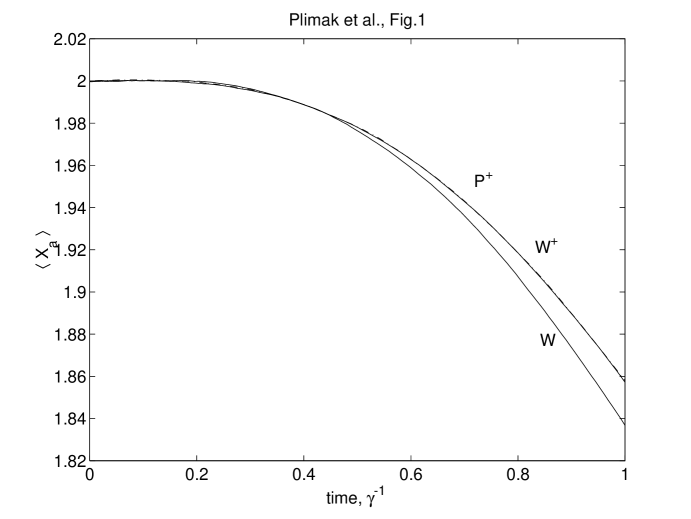
FIG. 1.: Predictions of the positive-W (upper solid line), positive-P (dashed line) and truncated Wigner (solid line) representations for quadrature relaxation in the OPO. We can see that the positive-P and positive-W solutions are almost indistinguishable.

REFERENCES

- [1] J.R. Klauder, in Proceedings of the Sixth International Conference on Path Integrals from peV to TeV, p. 65 (World Scientific, Singapore-New Jersey-London-Hong Kong, 1998)
- [2] C.W. Gardiner, Quantum Noise, Springer-Verlag, Berlin, (1991).
- [3] C.W. Gardiner, Handbook of Stochastic Methods, Springer-Verlag, Berlin, (1985).
- [4] M.J. Steel et al., Phys. Rev. A 58, 4824 (1998); P.D. Drummond and J.F. Corney, Phys. Rev. A 60, R2661 (1999); J.J. Hope and M.K. Olsen, Phys. Rev. Lett. 86, 3220 (2001); U. Poulsen and K. Molmer, Phys. Rev. A 63, 023604, (2001).
- [5] R.F. Pawula, Phys. Rev. 162, 186, (1967).
- [6] T.W. Marshall, Proc. R. Soc. London, Ser. A 276, 475, (1963).
- [7] P.D. Drummond and P. Kinsler, Phys. Rev. A 40, 4813, (1989); P. Kinsler and P.D. Drummond, Phys. Rev. A 43, 6194, (1991); Phys. Rev. A 44, 7848 (1991); D.T. Pope, P.D. Drummond and W.J. Munro, Phys. Rev. A 62, 042108 (2000); M.K. Olsen, K. Dechoum and L.I. Plimak, Opt. Commun. 190, 261, (2001); G.J. Milburn, Phys. Rev. A 33, 674, (1986).
- [8] M.K. Olsen, J.J. Hope and L.I. Plimak, Phys. Rev. A 64, 013601, (2001).
- [9] L.I. Plimak, M. Fleischhauer, M.K. Olsen and M.J. Collett, preprint cond-mat/0102483 (2001).
- [10] P.D. Drummond, C.W. Gardiner, J. Phys. A 13, 2353, (1980).
- [11] D.F. Walls and G.J. Milburn, Quantum Optics, Springer-Verlag, Berlin, (1995).
- [12] R.J. Glauber, Phys. Rev. 130, 2529, (1963); P.L. Kelly and W.H. Kleiner, Phys. Rev. 136, 316, (1964).
- [13] L.I. Plimak, M. Fleischhauer, M.J. Collett, and D.F. Walls, preprint cond-mat/9712192.
- [14] L.I. Plimak, M. Fleischhauer and D.F. Walls, Europhysics Letters 43, 641 (1998).
- [15] L.I. Plimak, M.J. Collett, D.F. Walls and M. Fleischhauer, in Proceedings of the Sixth International Conference on Path Integrals from peV to TeV, p. 241 (World Scientific, Singapore-New Jersey-London-Hong Kong, 1998).
- [16] O.V. Konstantinov and V.I. Perel, Zh.Eksp.Teor.Fiz. 39, 197 (1960) [Sov.Phys.JETP 12, 142 (1961)]; L.V. Keldysh, Zh.Eksp.Teor.Fiz. 47, 1515 (1964) [Sov.Phys.JETP 20, 1018 (1964)].
- [17] H.W. Wyld, Ann.Phys. 14, 143 (1961).
- [18] J.W. Negerle and H. Orland, Quantum Many-Particle Systems, (Addison Wesley, Reading, Mass., 1978).
- [19] H. Risken, The Fokker-Planck Equation, (Springer-Verlag, Berlin, 1984).
- [20] J.J. Longdell, MSc thesis, University of Auckland, unpublished.