The one-way quantum computer – a non-network model of quantum computation

Abstract

A one-way quantum computer ($\mbox{QC}_{\cal{C}}$) works by only performing a sequence of one-qubit measurements on a particular entangled multi-qubit state, the cluster state. No non-local operations are required in the process of computation. Any quantum logic network can be simulated on the $\mbox{QC}_{\cal{C}}$. On the other hand, the network model of quantum computation cannot explain all ways of processing quantum information possible with the $\mbox{QC}_{\cal{C}}$. In this paper, two examples of the non-network character of the $\mbox{QC}_{\cal{C}}\,\,$are given. First, circuits in the Clifford group can be performed in a single time step. Second, the $\mbox{QC}_{\cal{C}}$-realisation of a particular circuit –the bit-reversal gate– has no network interpretation.

1 Introduction

Recently, we introduced the concept of the “one-way quantum computer” in [1]. In this scheme, the whole quantum computation consists only of a sequence of one-qubit projective measurements on a given entangled state, a so called cluster state [2]. We called this scheme the “one-way quantum computer” since the entanglement in a cluster state is destroyed by the one-qubit measurements and therefore the cluster state can be used only once. In this way, the cluster state forms a resource for quantum computation. The set of measurements form the program. To stress the importance of the cluster state for the scheme, we will use in the following the abbreviation $\mbox{QC}_{\cal{C}}\,\,$for “one-way quantum computer”.

As we have shown in [1], any quantum logic network [3] can be simulated on the $\mbox{QC}_{\cal{C}}$. On the other hand, the quantum logic network model cannot explain all ways of quantum information processing that are possible with the $\mbox{QC}_{\cal{C}}$. Circuits that realise transformations in the Clifford group –which is generated by all the CNOT-gates, Hadamard-gates and $\pi/2$ phase shifts– can be performed by a $\mbox{QC}_{\cal{C}}\,\,$in a single step, i.e. all the measurements to implement such a circuit can be carried out at the same time. The best networks that have been found have a logical depth logarithmic in the number of qubits [4]. In a simulation of a quantum logic network by a one-way quantum computer, the temporal ordering of the gates of the network is transformed into a spatial pattern of the measurement directions on the resource cluster state. For the temporal ordering of the measurements there seems to be no counterpart in the network model. Further, not every measurement pattern that implements a larger circuit can be decomposed into smaller units, as can be seen from the example of the bit-reversal gate given in Section 3.2.

The purpose of this paper is to illustrate the non-network character of the $\mbox{QC}_{\cal{C}}\,\,$using two examples – first, the temporal complexity of circuits in the Clifford group, and second, the bit-reversal gate on the $\mbox{QC}_{\cal{C}}\,\,$which has no network interpretation.

2 Summary of the one-way quantum computer

In this section, we give an outline of the universality proof [1] for the $\mbox{QC}_{\cal{C}}\,\,$. For the one-way quantum computer, the entire resource for the quantum computation is provided initially in the form of a specific entangled state –the cluster state [2]– of a large number of qubits. Information is then written onto the cluster, processed, and read out from the cluster by one-particle measurements only. The entangled state of the cluster thereby serves as a universal “substrate” for any quantum computation. Cluster states can be created efficiently in any system with a quantum Ising-type interaction (at very low temperatures) between two-state particles in a lattice configuration. More specifically, to create a cluster state $|\phi\rangle_{\cal{C}}$, the qubits on a cluster ${\cal{C}}$ are at first all prepared individually in a state $|+\rangle=1/\sqrt{2}(|0\rangle+|1\rangle)$ and then brought into a cluster state by switching on the Ising-type interaction $H_{\mbox{\tiny{int}}}$ for an appropriately chosen finite time span $T$. The time evolution operator generated by this Hamiltonian which takes the initial product state to the cluster state is denoted by $S$.

The quantum state $|\phi\rangle_{\cal{C}}$, the cluster state of a cluster $\cal C$ of neighbouring qubits, provides in advance all entanglement that is involved in the subsequent quantum computation. It has been shown [2] that the cluster state $|\phi\rangle_{\cal C}$ is characterised by a set of eigenvalue equations

$$\sigma_{x}^{(a)}\bigotimes_{a^{\prime}\in ngbh(a)}\sigma_{z}^{(a^{\prime})}|\phi\rangle_{\cal C}=\pm|\phi\rangle_{\cal C},$$ (1)

where $ngbh(a)$ specifies the sites of all qubits that interact with the qubit at site $a\in{\cal C}$. The eigenvalues are determined by the distribution of the qubits on the lattice. The equations (1) are central for the proposed computation scheme. It is important to realise here that information processing is possible even though the result of every measurement in any direction of the Bloch sphere is completely random. The reason for the randomness of the measurement results is that the reduced density operator for each qubit in the cluster state is $\frac{1}{2}{\bf{1}}$. While the individual measurement results are irrelevant for the computation, the strict correlations between measurement results inferred from (1) are what makes the processing of quantum information possible on the $\mbox{QC}_{\cal{C}}$.

For clarity, let us emphasise that in the scheme of the $\mbox{QC}_{\cal{C}}\,\,$we distinguish between cluster qubits on ${\cal{C}}$ which are measured in the process of computation, and the logical qubits. The logical qubits constitute the quantum information being processed while the cluster qubits in the initial cluster state form an entanglement resource. Measurements of their individual one-qubit state drive the computation.

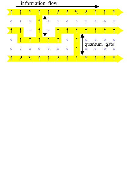
Figure 1: Quantum computation by measuring two-state particles on a lattice. Before the measurements the qubits are in the cluster state $|\phi\rangle_{\cal{C}}$ of (1). Circles $\odot$ symbolise measurements of $\sigma_{z}$, vertical arrows are measurements of $\sigma_{x}$, while tilted arrows refer to measurements in the x-y-plane.

To process quantum information with this cluster, it suffices to measure its particles in a certain order and in a certain basis, as depicted in Fig. 1. Quantum information is thereby propagated through the cluster and processed. Measurements of $\sigma_{z}$-observables effectively remove the respective lattice qubit from the cluster. Measurements in the $\sigma_{x}$-eigenbasis are used for “wires”, i.e. to propagate logical quantum bits through the cluster, and for the CNOT-gate between two logical qubits. Observables of the form $\cos(\varphi)\,\sigma_{x}\pm\sin(\varphi)\,\sigma_{y}$ are measured to realise arbitrary rotations of logical qubits. For cluster qubits to implement rotations, the basis in which each of them is measured depends on the results of preceding measurements. This introduces a temporal order in which the measurements have to be performed. The processing is finished once all qubits except a last one on each wire have been measured. The remaining unmeasured qubits form the quantum register which is now ready to be read out. At this point, the results of previous measurements determine in which basis these “output” qubits need to be measured for the final readout, or if the readout measurements are in the $\sigma_{x}$-, $\sigma_{y}$- or $\sigma_{z}$-eigenbasis, how the readout measurements have to be interpreted. Without loss of generality, we assume in this paper that the readout measurements are performed in the $\sigma_{z}$-eigenbasis.

Here, we review two points of the universality proof for the $\mbox{QC}_{\cal{C}}$: the realisation of the arbitrary one-qubit rotation as a member of the universal set of gates, and the effect of the randomness of the individual measurement results and how to account for them. For the realisation of a CNOT-gate see Fig. 2 and [1].

An arbitrary rotation $U_{R}\in SU(2)$ can be achieved in a chain of 5 qubits. Consider a rotation in its Euler representation

$$U_{R}(\xi,\eta,\zeta)=U_{x}(\zeta)U_{z}(\eta)U_{x}(\xi),$$ (2)

where the rotations about the $x$- and $z$-axis are $U_{x}(\alpha)=\displaystyle{\mbox{exp}\left(-i\alpha\frac{\sigma_{x}}{2}\right)}$ and $U_{z}(\alpha)=\displaystyle{\mbox{exp}\left(-i\alpha\frac{\sigma_{z}}{2}\right)}$. Initially, the first qubit is in some state $|\psi_{\mbox{\footnotesize{in}}}\rangle$, which is to be rotated, and the other qubits are in $|+\rangle$. After the 5 qubits are entangled by the time evolution operator $S$ generated by the Ising-type Hamiltonian, the state $|\psi_{\mbox{\footnotesize{in}}}\rangle$ can be rotated by measuring qubits 1 to 4. At the same time, the state is also transfered to site 5. The qubits $1\dots 4$ are measured in appropriately chosen bases, viz.

$${\cal{B}}_{j}(\varphi_{j})=\left\{\frac{|0\rangle_{j}+e^{i\varphi_{j}}|1\rangle_{j}}{\sqrt{2}},\,\frac{|0\rangle_{j}-e^{i\varphi_{j}}|1\rangle_{j}}{\sqrt{2}}\right\}$$ (3)

whereby the measurement outcomes $s_{j}\in\{0,1\}$ for $j=1\dots 4$ are obtained. Here, $s_{j}=0$ means that qubit $j$ is projected into the first state of ${\cal{B}}_{j}(\varphi_{j})$. In (3) the basis states of all possible measurement bases lie on the equator of the Bloch sphere, i.e. on the intersection of the Bloch sphere with the $x-y$-plane. Therefore, the measurement basis for qubit $j$ can be specified by a single parameter, the measurement angle $\varphi_{j}$. The measurement direction of qubit $j$ is the vector on the Bloch sphere which corresponds to the first state in the measurement basis ${\cal{B}}_{j}(\varphi_{j})$. Thus, the measurement angle $\varphi_{j}$ is equal to the angle between the measurement direction at qubit $j$ and the positive $x$-axis. For all of the gates constructed so far, the cluster qubits are either –if they are not required for the realisation of the circuit– measured in $\sigma_{z}$, or –if they are required– measured in some measurement direction in the $x-y$-plane. In summary, the procedure to implement an arbitrary rotation $U_{R}(\xi,\eta,\zeta)$, specified by its Euler angles $\xi,\eta,\zeta$, is this: 1. measure qubit 1 in ${\cal{B}}_{1}(0)$; 2. measure qubit 2 in ${\cal{B}}_{2}\left((-1)^{s_{1}+1}\xi\right)$; 3. measure qubit 3 in ${\cal{B}}_{3}\left((-1)^{s_{2}}\eta\right)$; 4. measure qubit 4 in ${\cal{B}}_{4}\left((-1)^{s_{1}+s_{3}}\zeta\right)$. In this way the rotation $U_{R}^{\prime}$ is realised:

$$U_{R}^{\prime}(\xi,\eta,\zeta)=U_{\Sigma}U_{R}(\xi,\eta,\zeta).$$ (4)

The random byproduct operator

$$U_{\Sigma}=\sigma_{x}^{s_{2}+s_{4}}\sigma_{z}^{s_{1}+s_{3}}$$ (5)

can be corrected for at the end of the computation, as explained next.

The randomness of the measurement results does not jeopardise the function of the circuit. Depending on the measurement results, extra rotations $\sigma_{x}$ and $\sigma_{z}$ act on the output qubits of every implemented gate, as in (4), for example. By use of the propagation relations

$$U_{R}(\xi,\eta,\zeta)\,\sigma_{z}^{s}\sigma_{x}^{s^{\prime}} = \sigma_{z}^{s}\sigma_{x}^{s^{\prime}}\,U_{R}((-1)^{s}\xi,(-1)^{s^{\prime}}\eta,(-1)^{s}\zeta),$$ (6)

$$\mbox{CNOT}(c,t)\,{\sigma_{z}^{(t)}}^{s_{t}}{\sigma_{z}^{(c)}}^{s_{c}}{\sigma_{x}^{(t)}}^{s_{t}^{\prime}}{\sigma_{x}^{(c)}}^{s_{c}^{\prime}} = {\sigma_{z}^{(t)}}^{s_{t}}{\sigma_{z}^{(c)}}^{s_{c}+s_{t}}{\sigma_{x}^{(t)}}^{s_{c}^{\prime}+s_{t}^{\prime}}{\sigma_{x}^{(c)}}^{s_{c}^{\prime}}\,\mbox{CNOT}(c,t),$$ (7)

these extra rotations can be pulled through the network to act upon the output state. There they can be accounted for by properly interpreting the $\sigma_{z}$-readout measurement results.

To summarise, any quantum logic network can be simulated on a one-way quantum computer. A set of universal gates can be realised by one-qubit measurements and the gates can be combined to circuits. Due to the randomness of the results of the individual measurements, unwanted byproduct operators are introduced. These byproduct operators can be accounted for by adapting measurement directions throughout the process. In this way, a subset of qubits on the cluster ${\cal{C}}$ is prepared as the output register. The quantum state on this subset of qubits equals that of the quantum register of the simulated network up to the action of an accumulated byproduct operator. The byproduct operator determines how the measurements on the output register are to be interpreted.

3 Non-network character of the $\mbox{QC}_{\cal{C}}\,\,$

3.1 Logical depth $D=1$ for circuits in the Clifford group

The Clifford group of gates is generated by the CNOT-gates, the Hadamard-gates and the $\pi/2$-phase shifts. In this section it is proved that the logical depth of circuits belonging to the Clifford group is $D=1$ on the $\mbox{QC}_{\cal{C}}$, irrespective of the number of logical qubits $n$. For a subgroup of the Clifford group, the group generated by the CNOT- and Hadamard gates we can compare the result to the best known upper bound for quantum logic networks where the logical depth scales like $O(\log n)$ [4].

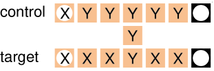
CNOT-gate	Hadamard-gate	$\pi/2$-phase gate

Figure 2: Realisation of the required gates on the $\mbox{QC}_{\cal{C}}$. CNOT-gate between neighbouring qubits, the Hadamard gate and the $\pi/2$ phase gate.

The Hadamard- and the $\pi/2$-phase gate are, compared to general $SU(2)$-rotations, special with regard to the measurements which are performed on the cluster to implement them. The Euler angles (2) that implement a Hadamard- and a $\pi/2$-phase gate are, depending on the byproduct operator on the input side, given by $\xi=\pm\pi/2,\,\,\eta=\pm\pi/2,\,\,\zeta=\pm\pi/2$ and $\xi=0,\,\,\eta=\pm\pi/2,\,\,\zeta=0$, respectively. See Fig. 2. A measurement angle of 0 corresponds to a measurement of the observable $\sigma_{x}$ and both measurement angles $\pi/2$ and $-\pi/2$ correspond to a measurement of $\sigma_{y}$. A change of the measurement angle from $\pi/2$ to $-\pi/2$ has only the effect of interchanging the two states of the measurement basis in (3), but it does not change the basis itself.

In general, cluster qubits which are measured in the eigenbasis of $\sigma_{x}$, $\sigma_{y}$ or $\sigma_{z}$ can be measured at the same time. The adjustment of their measurement basis does not require classical information gained by measurements on other cluster qubits. As described in [1], $\sigma_{z}$-measurements are used to eliminate those cluster qubits which are not essential for the circuit. As shown in Fig. 2, the cluster qubits essential for the implementation of the CNOT-gate between neighbouring qubits, the Hadamard- and the $\pi/2$-phase gate are all measured in the $\sigma_{x}$- or $\sigma_{y}$-eigenbasis. The general CNOT can be constructed from CNOT-gates between neighbouring qubits. This can be done in the standard manner using the swap-gate composed of three CNOT-gates. Hence also the general CNOT-gate requires only $\sigma_{x}$- and $\sigma_{y}$-measurements. Therefore, all circuits in the Clifford group can be realised in a single step of parallel measurements.

3.2 The bit-reversal gate

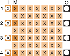
Figure 3: This measurement pattern implements a bit-reversal gate. Each square represents a lattice qubit. The squares in the extreme left column marked with white circles denote the input qubits, they on the right-most column denote the output qubits. Note that blank squares can represent either $\sigma_{z}$ measurements or empty lattice sites.

The measurement pattern shown in Fig. 3 realises a bit-reversal gate. In this example, it acts on four logical qubits, reversing the bit order, $|x_{3}x_{2}x_{1}x_{0}\rangle\to|x_{0}x_{1}x_{2}x_{3}\rangle$. Reconsidering the circuit of CNOT-gates and one-qubit rotations depicted in Fig. 1, the network structure –displayed in gray underlay– is clearly reflected in the measurement pattern. One finds the wires for logical qubits “isolated” from each other by areas of qubits measured in $\sigma_{z}$ and “bridges” between the wires which realise two-qubit gates.

For the bit-reversal gate in Fig. 3 the situation is different. To implement this gate on $n$ logical qubits, the cluster qubits on a square block of size $2n-1\,\times 2n-1$ all have to be measured in the $\sigma_{x}$-eigenbasis. The circuit which is realised via this measurement pattern cannot be explained by decomposing it into smaller parts. There is no network interpretation –as there is for Fig. 1– for the measurement pattern displayed in Fig. 3.

The bit reversal gate can be understood in a similar way to teleportation. Here we give an explanation for the bit-reversal gate on four qubits, but the argument can be straightforwardly generalised to an arbitrary number $n$ of logical qubits. In Fig. 3 we have the set of input qubits $I=\{i_{1},\dots,i_{4}\}$, their neighbouring qubits $M=\{m_{1},\dots,m_{4}\}$ and the set of output qubits $O=\{o_{1},\dots,o_{4}\}$. All the qubits required for the gate form the set $Q$. Further, we define the “body” G of the gate as the set $G=Q\backslash(I\cup M\cup O)$. As in [1], the standard setting to discuss a gate is the following: 1.) Prepare the input qubits $I$ in an input state $|\psi_{\mbox{\footnotesize{in}}}\rangle$ and the remaining qubits each in $|+\rangle$. 2.) Entangle the qubits in $Q$ by $S$, the unitary transformation generated by the Ising-interaction $H_{\mbox{\tiny{int}}}$. 3.) Measure the qubits in $I\cup M\cup G$, i.e. all but the output qubits, in the $\sigma_{x}$-eigenbasis. Due to linearity we can confine ourselves to input states of product form $|\psi_{\mbox{\footnotesize{in}}}\rangle=|\alpha\rangle_{i_{1}}\otimes|\beta\rangle_{i_{2}}\otimes|\gamma\rangle_{i_{3}}\otimes|\delta\rangle_{i_{4}}.$ The output state we get after step 3 in the above protocol is $|\psi_{\mbox{\footnotesize{out}}}\rangle=U_{\Sigma}\,\,|\delta\rangle_{o_{1}}\otimes|\gamma\rangle_{o_{2}}\otimes|\beta\rangle_{o_{3}}\otimes|\alpha\rangle_{o_{4}}$. There, the multi-local byproduct operator $U_{\Sigma}$ belongs to a discrete set and depends only on the results of the measurements.

The entanglement operation $S$ on the qubits in $Q$ can be written as a product $S=S_{MGO}\,S_{IM}$ where $S_{MGO}$ entangles the qubits in $M$,$G$ and $O$ and $S_{IM}$ entangles the input qubits in $I$ with their neighbours in $M$. $S_{MGO}$ and $S_{IM}$ commute. Further, let $P$ denote the projection operator which describes the set of measurements in step 2 of the above protocol. Then, the projector $P$ can be written as a product as well, $P=P_{G}\,P_{IM}$. There, $P_{G}$ denotes the projector associated with the measurements on the set $G$ of qubits, and $P_{IM}$ the projector associated with the measurements on $I$ and $M$. Now note that $P_{G}$ commutes with $S_{IM}$, because the two operators act non-trivially only on different subsets of qubits. Therefore, the above protocol is mathematically equivalent to the following one: $1^{\prime}$.) Prepare the input qubits $I$ in an input state $|\psi_{\mbox{\footnotesize{in}}}\rangle$ and the remaining qubits each in $|+\rangle$. $2^{\prime}$.) Entangle the qubits in $M$, $G$ and $O$ by $S_{MGO}$. $3^{\prime}$.) Measure the qubits in $G$. $4^{\prime}$.) Entangle the qubits in $I$ and $M$ by $S_{IM}$. And $5^{\prime}$.) Measure the qubits in $I$ and $M$.

The quantum state of the qubits in $I$, $M$ and $O$ after step $3^{\prime}$ in the second protocol is of the form $|\Psi\rangle_{IMO}=|\psi_{\mbox{\footnotesize{in}}}\rangle_{I}\otimes|\Phi\rangle_{MO}$. As a consequence of the eigenvalue equations (1) of the unmeasured state of the qubits in $M$, $G$ and $O$, the state $|\Phi\rangle_{MO}$ obeys the following set of eight eigenvalue equations: $\sigma_{x}^{(m_{1})}\sigma_{z}^{(o_{4})}\,|\Phi\rangle_{MO}=\pm|\Phi\rangle_{MO}$, $\sigma_{z}^{(m_{1})}\sigma_{x}^{(o_{4})}\,|\Phi\rangle_{MO}=\pm|\Phi\rangle_{MO}$, and the three remaining pairs of equations with $(m_{1},o_{4})$ replaced by $(m_{2},o_{3})$, $(m_{3},o_{2})$ and $(m_{4},o_{1})$. The sign factors in these equations depend on the results measured in step $3^{\prime}$ of the second protocol. The eigenvalue equations determine the state $|\Phi\rangle_{MO}$ completely. It is the product of four Bell states $|\mbox{B}\rangle$: $|\Phi\rangle_{MO}=_{\mbox{\scriptsize l.u.}}|\mbox{B}\rangle_{m_{1}o_{4}}\otimes|\mbox{B}\rangle_{m_{2}o_{3}}\otimes|\mbox{B}\rangle_{m_{3}o_{2}}\otimes|\mbox{B}\rangle_{m_{4}o_{1}}$, where $|\mbox{B}\rangle=1/\sqrt{2}(|+\rangle|1\rangle+|-\rangle|0\rangle)$ and “$=_{\mbox{\scriptsize l.u.}}$” means equal up to possible local unitarities $\sigma_{x},\sigma_{z}$ on the output qubits in $O$. The entanglement operation $S_{IM}$ in step $4^{\prime}$ together with the local measurements $P_{IM}$ in step $5^{\prime}$ has the effect of four Bell measurements on the qubit pairs $(i_{k},m_{k}),\;k=1\dots 4$, in the basis $\{1/\sqrt{2}(|0\rangle_{i_{k}}|\pm\rangle_{m_{k}}\pm|1\rangle_{i_{k}}|\mp\rangle_{m_{k}})\}$.

The second protocol –which is mathematically equivalent to the first– is thus a teleportation scheme. In steps $2^{\prime}$ and $3^{\prime}$ Bell pairs between intermediate qubits $m_{k}\in M$ and the output qubits are created. The first qubit in $M$ forms a Bell state with the last qubit in $O$, and so on:

In steps $4^{\prime}$ and $5^{\prime}$ a Bell measurement on each pair of qubits $(i_{k},m_{k})$ is performed. In this way, the input state $|\psi_{\mbox{\footnotesize{in}}}\rangle$ is teleported from the input to the output qubits, with the order of the qubits reversed. As in teleportation, the output state is equivalent to the input state only up to the action of a multi-local unitary operator which is specified by two classical bits per teleported qubit. In the case of the bit-reversal gate the role of this operator is taken by the byproduct operator $U_{\Sigma}$.

Please note that there is no temporal order of measurements here. All measurements can be carried out at the same time. The apparent temporal order in the second protocol was introduced only as a pedagogical trick to explain the bit-reversal gate in terms of teleportation.

4 Conclusion

In this paper, we have shown that the network picture cannot describe all ways of quantum information processing that are possible with a one-way quantum computer. First, circuits which realise unitary transformations in the Clifford group can be performed on the $\mbox{QC}_{\cal{C}}\,\,$in a single time step. This includes in particular all circuits composed of CNOT- and Hadamard gates, for which the best known network has a logical depth that scales logarithmically in the number of qubits. Second, we presented an example of a circuit on the $\mbox{QC}_{\cal{C}}$, the bit-reversal gate, which cannot be interpreted as a network composed of gates. These observations motivate a novel computational model underlying the $\mbox{QC}_{\cal{C}}$, which is described in [5].

References

- [1] R. Raussendorf and H.-J. Briegel, Phys. Rev. Lett. 86, 5188 (2001).
- [2] H.-J. Briegel and R. Raussendorf, Phys. Rev. Lett. 86, 910 (2001).
- [3] D. Deutsch, Proc. R. Soc. London Ser. A 425, 73 (1989).
- [4] C. Moore and M. Nilsson, quant-ph/9808027 (1998).
- [5] R. Raussendorf and H.-J. Briegel, quant-ph/0108067 (2001).