Present address: ]Harvard University, Maxwell Dworkin Laboratory, 33 Oxford Street, Cambridge, Massachusetts 02138

Polynomial-Time Simulation of Pairing Models on a Quantum Computer

Abstract

We propose a polynomial-time algorithm for simulation of the class of pairing Hamiltonians, e.g., the BCS Hamiltonian, on an NMR quantum computer. The algorithm adiabatically finds the low-lying spectrum in the vicinity of the gap between ground and first excited states, and provides a test of the applicability of the BCS Hamiltonian to mesoscopic superconducting systems, such as ultra-small metallic grains.

The potential of quantum computers (QCs) to provide exponential speed-up in the simulation of quantum physics problems was originally conjectured by Feynman Feynman:QC , confirmed by Lloyd Lloyd:96 , and later studied theoretically by a number of authors, e.g., Meyer:96Wiesner:96Zalka:98Boghosian:97aLidar:98RC ; Abrams:99 ; Abrams:97Ortiz:00 ; Bravyi:00 ; Dodd:01Wocjan:01 . NMR-QC experiments performing quantum physics simulations were reported in Somaroo:99Tseng:00 . Current QC technology is limited to fewer than 10 qubits and the testing of simple algorithms Knill:00a . QCs of the next generation, with 10-100 qubits, have the potential to solve hard problems in quantum many-body theory. We show here how this observation can be applied to the problem of simulating the class of pairing Hamiltonians with general, i.e., arbitrary long-range interactions. The pairing Hamiltonians are of wide interest in condensed matter and nuclear physics Mahan:bookRing:book . An important example of a pairing Hamiltonian is the BCS model of low-T_c superconductivity. We provide an algorithm for testing the validity of the general BCS Hamiltonians of finite particle-number systems, pertinent to nuclear systems and mesoscopic condensed-phase systems, such as ultra-small metallic grains Ralph:97 ; Mastellone:98 ; BraunDelft:98 ; Dukelsky:99 . These grains provide a fertile testing ground for the BCS ansatz for the ground state wave function. The BCS wave function is a superposition of different Fermion numbers and is expected to be exact in the thermodynamic limit Anderson:58 . In contrast, in ultra-small metallic grains the number of states $N$ within the Debye frequency cutoff from the Fermi energy is only $\sim 100$. A similar estimate holds for the number of states within a few major shells for medium or heavy nuclei. In systems with finite particle number the BCS ansatz is doubtful, and at the same time exact numerical diagonalization of the general BCS Hamiltonian is impractical beyond a few tens of electron pairs Mastellone:98 . Various approximations have been proposed Braun:98 , but it would clearly be desirable to have an exact numerical solution for the problem. In Abrams:97Ortiz:00 ; Bravyi:00 efficient QC algorithms were presented for simulating a many-body fermionic system. While the BCS Hamiltonian describes a system of interacting fermions, it does so at the level of an effective field theory. This can be expressed in terms of an interacting spin system Anderson:58 , or parafermions WuLidar1:01 . Therefore the fermionic simulation algorithms Abrams:97Ortiz:00 are not directly applicable. Further, while a number of authors have recently considered simulation of one Hamiltonian in terms of another Dodd:01Wocjan:01 , the connection of these phenomenological Hamiltonians to those of many-body condensed matter and nuclear physics is not a priori clear. Here we clarify the correspondence by proposing an explicit and numerically exact diagonalization algorithm that is suitable for general pairing Hamiltonians, and is directly implementable in NMR-type quantum computers Cory:00 . More generally, with minor modifications our algorithm is applicable to all QCs with short-range exchange-type interactions, such as quantum dots Burkard:00 . Using an adiabatic procedure, we show how to obtain only the low-lying energy spectrum, e.g., in the vicinity of the superconducting gap, with an algorithm that takes $\sim N^{4}$, instead of exponential, computational steps. The number of qubits we require equals the effective number of states $N$, so that a QC with $\sim 100$ qubits (neglecting overhead due to error correction) could solve a problem that is well out of the reach of current classical computers.

Mapping of Bosons and Fermions to Qubits.— Pairing Hamiltonians are typically expressed in terms of fermionic or bosonic creation (annihilation) operators, $c_{m}^{\dagger}$ ($c_{m}$) and $b_{m}^{\dagger}$ ($b_{m}$), respectively, where $|m|=1,2,\ldots,N$ denotes all relevant quantum numbers. E.g., the general BCS pairing Hamiltonian has the form:

$$H_{\mathrm{BCS}}=\sum_{m=1}^{N}\frac{\epsilon_{m}}{2}(n_{m}^{F}+n_{-m}^{F})+\sum_{m,l=1}^{N}V_{ml}^{+}c_{m}^{\dagger}c_{-m}^{\dagger}c_{-l}c_{l}$$

where $n_{\pm m}^{F}\equiv c_{\pm m}^{\dagger}c_{\pm m}$ is the number operator, and the matrix elements $V_{ml}^{+}\equiv\left\langle m,-m\right|V\left|l,-l\right\rangle$ (we impose no restriction on $m,l$) are real and can be calculated, e.g., for superconductors, in terms of the Coulomb force and the electron-phonon interaction Mahan:bookRing:book . Pairs of fermions are labeled by the quantum numbers $m$ and $-m$, according to the Cooper pair situation where paired electrons have equal energies but opposite momenta and spins: $m=(\mathbf{p},\uparrow)$ and $-m=(-\mathbf{p},\downarrow)$. These are degenerate, time-reversed partners whose energies are considered phenomenological parameters Braun:98 . The same idea is applicable to nuclei, where effective pairings occur between nucleons in time-reversed partners Mahan:bookRing:book . $N$ is an effective state number, which equals the number of qubits in the algorithm below. E.g., in the case of metallic grains $N$ is twice the the Debye frequency in units of the average level spacing (inversely proportional to volume of the grain). For nuclear pairing models, $N$ could be the number of states in one or more major energy shells.

To make a connection to quantum algorithms we map the fermionic or bosonic operators to qubit operators. We denote the raising and lowering operators for the $m^{\mathrm{th}}$ qubit by the Pauli matrices $\sigma_{m}^{\pm}$, acting non-trivially only on the $m^{\mathrm{th}}$ qubit. A “number operator” is $n_{m}=(\sigma_{m}^{z}+1)/2$, where $n_{m}=1$ ($0$) if the $m^{\mathrm{th}}$ qubit is in state $|1\rangle$ ($|0\rangle$); $n=\sum_{m}n_{m}$ is the number of 1’s in a computational basis state (a ket of a single bit-string), and will correspond, e.g., to the number of Cooper pairs in our applications below. The computational ground state $\left|\mathtt{0}\right\rangle=\left|0_{1}0_{2}\cdots 0_{N}\right\rangle$ acts as a vacuum state: $n\left|\mathtt{0}\right\rangle=\sigma_{m}^{-}\left|\mathtt{0}\right\rangle=0$. Now we can consider three generic pairing cases and map them to qubits. In each case we identify fermionic or bosonic operator pairs that satisfy the commutation rules of $sl(2)=\{\sigma_{m}^{+},\sigma_{m}^{-},\sigma_{m}^{z}\}$ (see WuLidar1:01 for details). These cases are: (i) Fermionic particle-particle pairs (e.g., Cooper pairs): $sl(2)=\{c_{-m}c_{m},c_{m}^{\dagger}c_{-m}^{\dagger},n_{m}^{F}+n_{-m}^{F}-1\}$, provided $n_{m}^{F}=n_{-m}^{F}$ (a condition satisfied by $H_{\mathrm{BCS}}$), and $\left|\mathtt{0}\right\rangle=\left|\mathtt{0}\right\rangle_{F}$. (ii) Fermionic particle-hole pairs (e.g., excitons):$\ sl(2)=\{c_{-m}^{\dagger}c_{m},c_{m}^{\dagger}c_{-m},n_{m}^{F}-n_{-m}^{F}\}$, provided $n_{m}^{F}+n_{-m}^{F}=1$ and $\left|\mathtt{0}\right\rangle=c_{-N}^{\dagger}\cdots c_{-2}^{\dagger}c_{-1}^{\dagger}\left|\mathtt{0}\right\rangle_{F}$ . (iii) Bosonic ‘particle-hole’ pairs (e.g., dual-rail photons in the optical quantum computer proposal Knill:00 ): $sl(2)=\{b_{-m}^{\dagger}b_{m},b_{m}^{\dagger}b_{-m},n_{m}^{B}-n_{-m}^{B}\}$, provided $n_{m}^{B}+n_{-m}^{B}=1$ and $\left|\mathtt{0}\right\rangle=b_{-N}^{\dagger}\cdots b_{-2}^{\dagger}b_{-1}^{\dagger}\left|\mathtt{0}\right\rangle_{B}$. The three conditions above each restrict the dynamics to a different subspace of the entire Hilbert space. The conditions play the role of conserved quantities and only Hamiltonians that satisfy them preserve such subspaces.

It is now clear how to express $H_{\mathrm{BCS}}$ in terms of qubit operators. In fact, a more general Hamiltonian, that is applicable to all cases (i)-(iii) is:

$$H_{\mathrm{p}}=\sum_{m=1}^{N}\frac{\varepsilon_{m}}{2}\sigma_{m}^{z}+\sum_{r=\pm}\sum_{l>m=1}^{N}\frac{V_{ml}^{r}}{2}(\sigma_{m}^{x}\sigma_{l}^{x}+r\sigma_{m}^{y}\sigma_{l}^{y}),$$ (1)

where $\varepsilon_{m}=\epsilon_{m}+V_{mm}^{+}$ and $V_{ml}^{-}=0$ for $H_{\mathrm{BCS}}$; $l,m$ now denote both state indices and qubit indices. Further, in the BCS case the qubit state space $\mathcal{H}_{P}=\mathrm{Span}\{\left|\mathtt{0}\right\rangle,\sigma_{m}^{+}\left|\mathtt{0}\right\rangle,\sigma_{l}^{+}\sigma_{m}^{+}\left|\mathtt{0}\right\rangle,\cdots\}$ is mapped into a subspace of the total fermionic Hilbert space where $n_{m}^{F}=n_{-m}^{F}$. $H_{\mathrm{BCS}}$ conserves the total number operator $n$ (the number of Cooper pairs). In terms of qubits, this means that the number of $|1\rangle$’s in a general $N$-qubit state is fixed by $H_{\mathrm{BCS}}$. Thus the Hilbert space splits into invariant subspaces with dimension ${\ {\binom{N}{n}}}$ for fixed $n$. The problem is reduced to diagonalizing separate blocks of size ${\ {\binom{N}{n}}}$. For half-filled states in a system with $N=100$, an exact solution could require diagonalizing a $10^{29}\times 10^{29}$-dimensional matrix. Such a task is clearly unfeasible on a classical computer.

Simulation of $H_{\mathrm{p}}$.— For concreteness and direct contact with feasible experiments, we limit our discussion of the simulation of $H_{\mathrm{p}}$ to the nearest-neighbor Ising-type Hamiltonian of NMR: $H_{\mathrm{NMR}}=\sum_{l=1}^{N}\frac{\omega_{l}}{2}\sigma_{l}^{z}+\sum_{l=1}^{N-1}J_{l}\sigma_{l}^{z}\sigma_{l+1}^{z}$, supplemented with external single qubit operations $F=\sum_{l=1}^{N}f_{l}^{x}\sigma_{l}^{x}+f_{l}^{y}\sigma_{l}^{y}$. The same Hamiltonian describes, e.g., a QC implementation using coupled Josephson junctions Blais:00 . We emphasize that this simulation is also directly implementable in systems that use exchange-type interactions, since the logical operations for those systems are equivalent (up to polynomial overhead) to those using the Ising coupling Dodd:01Wocjan:01 ; WuLidar1:01 . We shall for simplicity only explicitly discuss the case $V_{ml}^{-}=0$, but the same procedure will apply also to the case of $V_{ml}^{-}\neq 0$ (since the two cases are related by a simple unitary transformation). From now on we denote $V_{ml}^{+}\equiv V_{ml}$.

Below, we develop an explicit polynomial-time algorithm for simulating $\{U_{\mathrm{p}}(k\tau)=\exp(-iH_{\mathrm{p}}k\tau)\}_{k=1}^{T/\tau}$ ($\tau$, $T$ are defined later). This sequence can be Fourier-transformed and the spectrum of $H_{\mathrm{p}}$ found Abrams:99 . However, although this may be achieved directly using NMR methods, we are primarily interested in the low-lying spectrum (e.g., in the BCS case, near the superconducting gap). Our algorithm therefore includes an adiabatic component, that allows us to probe just this part of the spectrum. Let us now outline the main steps in our algorithm for simulating $H_{\mathrm{p}}$ using $H_{\mathrm{NMR}}$ and $F$. (i) Prepare a computational basis state $|x_{n}\rangle$ with fixed $n$ (number of $|1\rangle$’s). This step is well-known and needs no further explanation Cory:00 . (ii) Quasi-adiabatically evolve $|x_{n}\rangle$ to $|\psi(0)\rangle_{0}=|g_{n}\rangle+\theta|e_{n}\rangle$: an approximate ground state of $H_{\mathrm{p}}$ ($|g_{n}\rangle$ is an exact ground state, $|e_{n}\rangle$ is a first excited state and $\theta\ll 1$), with the same $n$ as $|x_{n}\rangle$. (iii) Rotate $|\psi(0)\rangle_{0}$ to $|\psi(0)\rangle=|g_{n,n\pm 1}\rangle+\theta^{\prime}|e_{n,n\pm 1}\rangle$, a state that includes contributions from $n\pm 1$ as well. (iv) Implement $U_{\mathrm{p}}(t)=\exp(-iH_{\mathrm{p}}t)$ on $|\psi(0)\rangle$. (v) Measure. Repeat steps (i)-(v) while increasing $t$ in step (v). We describe each of these steps in detail, starting for simplicity from step (iv).

Step (iv): Implementation of $\exp(-iH_{\mathrm{p}}t)$.— In NMR one can only control $f_{l}^{x}$ (or $f_{l}^{y}$) directly, while all $\omega_{l},J_{l}$ are always on Cory:00 . Also, $J_{l}$ usually is positive. A powerful method that allows us to deal with such constraints (that are not unique to NMR) is recoupling (e.g., Leung:00 ). The idea is based on elementary angular momentum theory. We define $C_{A}^{\varphi}\circ e^{i\theta B}\equiv e^{i\varphi A}e^{i\theta B}e^{-i\varphi A}$, where $A,B$ are generators of $su(2)$ (e.g., two Pauli matrices), and/or $\{A,B\}=0$ while $A^{2}=\mathbf{1}$. This recoupling sequence can be interpreted as the application of time-reversed pulses ($e^{\pm i\varphi A}$) before and after periods of free evolution $e^{i\theta B}$. Special cases of interest are (i) $C_{A}^{\pi/2}\circ e^{i\theta B}=e^{-i\theta B}$, (ii) $C_{A}^{\pi/4}\circ e^{i\theta B}=e^{i\theta(iBA)}$. Thus, to obtain evolution under $\frac{\omega_{l}}{2}\sigma_{l}^{z}$ we apply the (unoptimized) recoupling sequence $\exp(-\frac{i\omega_{l}}{2}\sigma_{l}^{z}t)=(e^{-iH_{\mathrm{NMR}}t/4}T_{l}e^{-iH_{\mathrm{NMR}}t/4}T_{l}^{\prime})^{2}$, where $T_{l}=\otimes_{j\neq l}\sigma_{j}^{x}$, $T_{l}^{\prime}=\otimes_{j\neq l}^{\prime}\sigma_{j}^{x}$ where the prime indicates that $j$ is even (odd) if $l$ is even (odd). This takes $3N$ pulses. Fig. 1(a) illustrates an optimized circuit for $N=2$. Similarly, we can evolve under any term $\sigma_{j}^{z}\sigma_{j+1}^{z}$ using $\sim 7N$ recoupling steps.

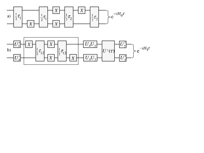
Figure 1: Quantum circuits to simulate $e^{-iH_{0}\tau}$ (a) and $e^{-iH_{I}\tau}$ (b) for the two qubit case. Time flows from left to right. $X\equiv\sigma^{x}$. The recoupling procedure yielding $U^{z}(\tau)=\exp(-iJ_{1}\tau_{12}\sigma_{1}^{z}\sigma_{2}^{z})$ is in the box in (b), and is repeated without detail. We set $\omega_{i}\tau_{i}=\varepsilon_{i}\tau$ ($i=1,2$) and $2J_{1}\tau_{12}=\left|V_{12}\right|\tau$. Rectangular boxes connecting two qubits denote evolution under $H_{\text{{NMR}}}$ for the indicated time.

Next, we need to show how to simulate long-range interactions using $H_{\mathrm{NMR}}$ and $F$. The set $\{X_{lm}\equiv\frac{1}{2}\left(\sigma_{l}^{x}\sigma_{m}^{x}+\sigma_{l}^{y}\sigma_{m}^{y}\right),Y_{lm}\equiv\frac{1}{2}\left(\sigma_{l}^{y}\sigma_{m}^{x}-\sigma_{l}^{x}\sigma_{m}^{y}\right),Z_{lm}\equiv\frac{1}{2}\left(\sigma_{l}^{z}-\sigma_{m}^{z}\right)\}$ forms an $su(2)$ algebra, and commutes with $\sigma_{m}^{z}+\sigma_{l}^{z}$ for any $l,m$ WuLidar:01 . Thus $C_{X_{ll+1}}^{\pi/2}\circ Z_{l,l+1}=-Z_{l,l+1}$, while $C_{X_{ll+1}}^{\pi/2}\circ(\sigma_{l}^{z}+\sigma_{l+1}^{z})=(\sigma_{l}^{z}+\sigma_{l+1}^{z})$. Adding yields $C_{X_{ll+1}}^{\pi/2}\circ\left(\sigma_{l-1}^{z}\sigma_{l}^{z}\right)=\sigma_{l-1}^{z}\sigma_{l+1}^{z}$, so that $C_{X_{ll+1}}^{\pi/2}\circ e^{i\theta\sigma_{l-1}^{z}\sigma_{l}^{z}}=e^{i\theta\sigma_{l-1}^{z}\sigma_{l+1}^{z}}$. Thus $C_{X_{ll+1}}^{\pi/2}$ acts as a nearest-neighbor exchange operator. In order to implement $C_{X_{ll+1}}^{\pi/2}$ using $H_{\mathrm{NMR}}$ and $F$ note that:

$$e^{-i\frac{\pi}{2}X_{ll+1}}=C_{\sigma_{l}^{x}+\sigma_{l+1}^{x}}^{-\pi/4}\circ e^{{-i\frac{\pi}{4}\sigma_{l}^{z}\sigma_{l+1}^{z}}}\,C_{\sigma_{l}^{y}+\sigma_{l+1}^{y}}^{\pi/4}\circ e^{{-i\frac{\pi}{4}\sigma_{l}^{z}\sigma_{l+1}^{z}}}.$$

It is simple to check that to create all possible couplings $\sigma_{l}^{z}\sigma_{m}^{z}$ in this manner requires $O(N^{3})$ steps. This procedure allows us to use the short-range NMR Hamiltonian to simulate $J_{l}\sigma_{l}^{z}\sigma_{m}^{z}$ with $|l-m|$ arbitrary. Let us now show how to turn this into a simulation of $H_{I}\equiv\frac{1}{2}\sum_{l>m=1}^{N}V_{ml}(\sigma_{m}^{x}\sigma_{l}^{x}+\sigma_{m}^{y}\sigma_{l}^{y})$. Suppose that $H_{\mathrm{p}}$ evolves for time $\tau$. We can turn on $-J_{l}\sigma_{l}^{z}\sigma_{m}^{z}$ for a time $\tau_{ml}$ such that $2J_{l}\tau_{ml}=|V_{ml}|\tau$ (for a BCS Hamiltonian $V_{ml}<0$). Doing this for all couplings separately (in series) shows that the evolution operator $U^{z}(\tau)=\exp(-\frac{i}{2}\sum_{l>m}V_{lm}\sigma_{l}^{z}\sigma_{m}^{z}\tau)$ is obtained using the same $O(N^{3})$ steps. By adjusting single-qubit operation times, we can implement $U^{\alpha}=\exp(i\frac{\pi}{4}\sum_{l}\sigma_{l}^{\alpha})$, to yield: $\exp(-iH_{I}\tau)=\left(U^{x\dagger}U^{z}(\tau)U^{x}\right)\left(U^{y}U^{z}(\tau)U^{y\dagger}\right)$, using $O(N^{3})$ steps. However, $H_{\mathrm{p}}$ also contains the term $H_{0}\equiv$$\sum_{l=1}^{N}\frac{\varepsilon_{l}}{2}\sigma_{l}^{z}$, which does not commute with $H_{I}$. Clearly, by turning on single qubit NMR $\sigma_{l}^{z}$ terms for times $\tau_{l}$ so that $\omega_{l}\tau_{l}=\varepsilon_{l}\tau$, we can simulate $H_{0}$ directly using $N$ steps. The non-commutativity implies that we need a short-time approximation in order to simulate the full $U_{\mathrm{p}}(\tau)=\exp(-iH_{\mathrm{p}}\tau)$:

$$U_{\mathrm{p}}(\tau)=e^{-iH_{0}\tau}e^{-iH_{I}\tau}+O(\tau^{2}).$$ (2)

When the additional recoupling steps needed to turn off unwanted interactions (which we ignored above) are taken into account, using the method of Leung:00 , we find that $U_{\mathrm{p}}(\tau)$ requires a total of $\allowbreak s(N)=-\frac{4}{3}N^{2}+\frac{32}{3}N-\frac{47}{3}N^{3}+\frac{28}{3}N^{4}$ steps. This result may be improved somewhat if parallel operations are allowed. E.g., in Fig. 1 we show optimized circuits implementing $e^{-iH_{0}\tau}$ and $e^{-iH_{I}\tau}$ for $N=2$ qubits. If $H_{\mathrm{NMR}}$ contains beyond-nearest-neighbor interactions then at most $O(N^{5})$ steps are needed. The effect of the $O(\tau^{2})$ errors in quantum algorithms due to the short-time approximation has been analyzed, e.g., in Dodd:01Wocjan:01 . By concatenating short-time evolution segments one can then obtain the finite time ($k\tau=t$) evolution operator $U_{\mathrm{p}}(t)\approx(U_{\mathrm{p}}(\tau))^{k}$ Abrams:99 , in a total of $k\,s(N)$ steps.

Step (ii): Adiabatic Evolution.— Let $2\Delta$ be the gap between the ground and the first excited states, and let $0\leq c(t)\leq 1$, $c(0)=0$, $c(T)=1$, be a slowly varying function, i.e., $2\pi/T\ll 2\Delta$ (e.g., $c(t)=t/T$). Consider the time-ordered evolution $U_{\mathrm{ad}}(t)=\mathcal{T}\exp(-i\int_{0}^{t}H(s)ds)$ under a time-dependent Hamiltonian $H(t)=H_{0}+c(t)H_{I}$. For sufficiently small $\tau$ this factors into a product

$$U_{\mathrm{ad}}(k\tau)\approx e^{-iH(k\tau)\tau}\cdots e^{-iH(2\tau)\tau}e^{-iH(\tau)\tau}+O(\tau^{2}),$$ (3)

where $\exp(-iH(j\tau)\tau)\approx\exp(-iH_{0}\tau)\exp(-ic(j\tau)H_{I}\tau)$ ($j=1,...,k$), and now we choose times $\tau_{ml}(j)$ (for turning on $-J_{l}\sigma_{l}^{z}\sigma_{m}^{z}$) such that $2J_{l}\tau_{ml}()=|V_{ml}|\tau\,c(j\tau)$. Since $c(t)$ is slow, $U_{\mathrm{ad}}(k\tau)$ will represent an adiabatic evolution. The adiabatic theorem then ensures that the system will be in an eigenstate of $H_{\mathrm{p}}=H(T)$ at $T=k\tau$, provided the initial state is in an eigenstate of $H_{0}$. Moreover, this will be a ground state $|g_{n}\rangle$ of $H_{\mathrm{p}}$ (a state with fixed $n$) if the initial state is the ground state of $H_{0}$ (a computational basis state $|x_{n}\rangle$) comment . In order to probe the low-lying spectrum we may slightly relax the adiabatic condition $\pi/T\ll\Delta$, or $k\gg\pi/(\tau\Delta)$. This can be defined in terms of the adiabatic expansion where the first order constraint is the usual adiabatic assumption. Here we only wish to satisfy the second order condition Wu:89 . Then we obtain a state $|\psi(0)\rangle_{0}\approx|g_{n}\rangle+\theta|e_{n}\rangle$ which contains a small ($\theta\ll 1$) component $|e_{n}\rangle$ of some of the low-lying excited states of $H_{\mathrm{p}}$ (with the same $n$).

Steps (iii),(v): Measuring the Spectrum.— In NMR one measures the free-induction-decay (FID) signal, given by $V_{\alpha}(t)\propto\mathrm{Tr}(\rho(t)\sigma_{\alpha}^{-})$, where $\rho(t)$ is the system density matrix and $\alpha$ is the index of the measured spin (qubit) Cory:00 . To probe states with different $n$, we rotate to $|\psi(0)\rangle=e^{-i\omega\sigma_{\alpha}^{y}}|\psi(0)\rangle_{0}\approx|g_{n,n\pm 1}\rangle+\theta^{\prime}|e_{n,n\pm 1}\rangle$, where $\theta^{\prime},\omega\ll 1$, a state that includes contributions from $n\pm 1$ as well [step (iii)]. This is simple to do using the method of step (iv). Combining steps (ii)-(iv), we have $\rho(t)=U_{\mathrm{p}}(t)|\psi(0)\rangle\langle\psi(0)|U_{\mathrm{p}}^{\dagger}(t)$. To relate $V_{\alpha}(t)$ to the spectrum of the pairing Hamiltonian we introduce an appropriate basis. A complete set of conserved quantum numbers are the number of Cooper pairs $n$ (= the number of $1$’s in a computational basis state, lowered by $\sigma_{\alpha}^{-}$), the energy $E_{n,i}$ for fixed $n$, and a state degeneracy index $\beta_{i}$. Thus our basis states are labeled by $|n,i,\beta_{i}\rangle$ and $\rho(t)$ can be expanded as $\sum B_{n,i,\beta_{i}}B_{m,j,\beta_{j}}^{\ast}|n,i,\beta_{i}\rangle e^{i(E_{m,j}-E_{n,i})t}\langle m,j,\beta_{j}|$ with $|\psi(0)\rangle=\sum_{n,i,\beta_{i}}B_{n,i,\beta_{i}}|n,i,\beta_{i}\rangle$. We have

$$V_{\alpha}(t)\propto\sum_{m,n}\sum_{i,j}C_{m,j;n,i}^{(\alpha)}e^{i(E_{m,j}-E_{n,i})t},$$ (4)

where $C_{m,j;n,i}^{(\alpha)}\equiv\sum_{\beta_{i}\beta_{j}}B_{n,i,\beta_{i}}B_{m,j,\beta_{j}}^{\ast}\langle m,j,\beta_{j}|\sigma_{\alpha}^{-}|n,i,\beta_{i}\rangle$ $\propto$$\delta_{m,n-1}$. Fourier transforming, we obtain the energy spectrum $S(\omega)=\sum_{n,i,j}\tilde{C}_{n-1,j;n,i}^{(\alpha)}\delta(\omega-(E_{n-1,j}-E_{n,i}))$, with the gap defined as $2\Delta_{n}\equiv E_{n,1}-E_{n,0}$. Ideally, $\Delta_{n}$ can be found from a few runs with different initial $n$. There are two complications in practice: (i) Finding $\Delta_{n}$ in this manner depends on the coefficients $\tilde{C}_{n-1,j;n,i}^{(\alpha)}$ not vanishing. By measuring all qubits $\alpha$, it is likely that sufficiently many non-zero coefficients will be available. (ii) The sharpness of the $\delta$ functions depends on how densely the signal $V_{\alpha}(t)$ is sampled. To resolve the gap, we will need to sample with a resolution $\Delta\omega=2\pi/T<\Delta_{n}$. Recall that $H_{\mathrm{BCS}}$ conserves $n$. Thus the number of $\tau$-intervals required for fixed $n$ is $k(n)\gg\pi/(\tau\Delta_{n})$, which is just the adiabatic condition again. A total of $\frac{1}{2}k(n)^{2}$ elementary evolutions steps, each simulating evolution under $H_{\mathrm{p}}$ for length $\tau$, will thus be needed to simulate $\{U_{\mathrm{p}}(k\tau)\}_{k=1}^{T/\tau}$, and each such step takes $s(N)$ logic gates. The longest single run takes $k(n)s(N)$ steps, while $\frac{1}{2}k(n)^{2}s(N)$ is the total run-time of the algorithm. if the algorithm is to succeed in the absence of error correction, then we must have $k(n)s(N)<T_{2}/\tau_{\mathrm{\log ic}}$, the ratio of decoherence to logic gate time. For NMR, $T_{2}/\tau_{\mathrm{\log ic}}$ can be $\sim 10^{5}$. To estimate $k(n)$ we need $\tau$ and $\Delta_{n}$. The gap can be estimated experimentally, for nuclear and BCS systems using material dependent parameters Mahan:bookRing:book ; Ralph:97 . Recall that $\tau$ is related to the short-time approximation which allowed us to neglect commutator terms in the expansion of $U_{\mathrm{ad}}(t)$. Since $e^{\left(A+B\right)\tau}\approx e^{A\tau}e^{B\tau}e^{-\frac{1}{2}[A,B]\tau^{2}}$, we need to estimate when $|[A,B]\tau|\ll\min(|A|,|B|)$. To obtain a rough estimate we consider a reduced BCS model Dukelsky:99 : $V_{ml}\equiv-V<0$, $\varepsilon_{l}=\varepsilon_{0}+ld$. In the BCS case the level spacing $d\ll V$, but $\varepsilon_{0}\gg V$. Letting $A=\varepsilon_{l}\sigma_{l}^{z}$, $B=VX_{lm}$, we have $|[A,B]|=|V\left(\varepsilon_{l}-\varepsilon_{m}\right)Y_{lm}|>Vd$, while $\min(|A|,|B|)=V$. Thus the short-time approximation is valid when $\tau\ll 1/d.$ Using $k(n)\gg\pi/(\tau\Delta_{n})$ and $s(N)\approx 9N^{4}$ we thus have $k(n)\,s(N)\gg 30\frac{d}{\Delta_{n}}N^{4}$. In the BCS case $d/\Delta_{n}\ll 1$. Assuming $d/\Delta_{n}=0.1$ we find $k(n)\,s(10)\gg 3\times 10^{4}$, so that a simulation with $N\leq 10$ qubits seems to be within the reach of present day NMR simulations Cory:00 .

In order to illustrate the algorithm, consider a simple example, the circuit for which is given in Fig. 1. When $N=2$ the computational basis states are: $\{\left|00\right\rangle,\left|01\right\rangle,\left|10\right\rangle,\left|11\right\rangle\}$, with $n=0,1,1,2$ Cooper pairs, respectively. Diagonalizing $H_{\mathrm{p}}$ yields the energy spectrum: $\{E_{n}\}=\{E_{0}=-(\varepsilon_{1}+\epsilon_{2})/2,E_{1}^{\pm}=\pm\sqrt{\epsilon^{2}+V^{2}},E_{2}=(\varepsilon_{1}+\epsilon_{2})/2\}$. Steps (ii)-(v) of the algorithm can be carried out analytically. Fourier transforming the FID signal yields four spectral lines from which, e.g., the $n=1$ gap can be found as $2\Delta_{1}=E_{1}^{+}-E_{1}^{-}$.

Conclusions.— We have proposed an efficient algorithm for finding the low-lying spectrum of pairing models with arbitrary long-range interactions, such as the BCS Hamiltonian. This establishes a link between quantum computers (QCs) of the next generation (10-100 qubits) and outstanding problems in finite-system quantum physics, such as the applicability of the BCS model to mesoscopic solid-state and nuclear systems. It would be interesting to implement the algorithm using current NMR-QC know-how, thus extending the experimental repertoire of QC physics simulations Somaroo:99Tseng:00 .

D.A.L. gratefully acknowledges financial support from PREA, NSERC, and the Connaught Fund.

References

(1) R.P. Feynman, Intl. J. Theor. Phys. 21, 467
(1982).
(2) S. Lloyd, Science 273, 1073 (1996).
(3) D.A. Meyer, J.
Stat. Phys. 85, 551 (1996); S. Wiesner, eprint quant-ph/9603028; C. Zalka
, Proc. Roy. Soc. London Ser. A 454, 313 (1998); D.A. Lidar and H.
Wang, Phys. Rev. E 59, 2429 (1998).
(4) D.S. Abrams and S. Lloyd, Phys. Rev. Lett. 83,
5162 (1999).
(5) D.S. Abrams and S. Lloyd, Phys. Rev. Lett.
79, 2586 (1997); G. Ortiz et al., Phys. Rev. A 64,
022319 (2001).
(6) S. Bravyi and A. Kitaev, eprint quant-ph/0003137.
(7) J.L. Dodd et al., eprint
quant-ph/0106064; P. Wocjan et al., eprint quant-ph/0106077.
(8) S. Somaroo et al., Phys. Rev.
Lett. 82, 5381 (1999); C.H. Tseng et al., Phys. Rev. A. 61 , 012302 (2000).
(9) E. Knill et al., Nature 404, 368 (2000).
(10) G.D. Mahan, Many-Particle Physics,
3rd ed. (Kluwer, New York, 2000); P. Ring and P. Schuck, The
Nuclear Many-Body Problem (Springer, New York, 1980).
(11) D.C. Ralph et al., Phys. Rev. Lett. 78,
4087 (1997).
(12) A. Mastellone et al., Phys. Rev. Lett. 80, 4542 (1998).
(13) F. Braun and J. von Delft, Phys. Rev. Lett. 81 , 4712 (1998).
(14) J. Dukelsky and G. Sierra, Phys. Rev. Lett. 83,
172 (1999).
(15) P.W. Anderson, Phys. Rev. 112, 1900 (1958).
(16) P.A. Braun et al., Eur. Phys. J. D 2, 165
(1998).
(17) L.-A. Wu and D.A. Lidar, eprint quant-ph/0109078.
(18) D.G. Cory et al., Forts. Phys. 48, 875 (2000).
(19) G. Burkard et al., Forts. Phys. 48
965 (2000).
(20) E. Knill et al., Nature 409, 46 (2001).
(21) A. Blais and A.M. Zagoskin, Phys. Rev. A 61,
042308 (2000).
(22) D.W. Leung et al., Phys. Rev. A 61, 042310
(2000).
(23) L.-A. Wu and D.A. Lidar, Phys. Rev. A 65, 042318 (2002).
(24) A similar
adiabatic approach has been proposed recently as an alternative to the
standard circuit model of quantum computation, by
E. Farhi et al., eprint quant-ph/0001106.