Classicality of quantum information processing

Abstract

The ultimate goal of the classicality program is to quantify the amount of quantumness of certain processes. Here, classicality is studied for a restricted type of process: quantum information processing (QIP). Under special conditions, one can force some qubits of a quantum computer into a classical state without affecting the outcome of the computation. The minimal set of conditions is described and its structure is studied. Some implications of this formalism are the increase of noise robustness, a proof of the quantumness of mixed state quantum computing and a step forward in understanding the very foundation of QIP.

I Introduction

It is known thanks to Bernstein and Vazirani BV1993 that, in a realistic context where errors occur and finite probability of success is accepted, quantum mechanics offers greater computational power than classical mechanics for some oracle types of problem. It was then shown by Simon simon1994 that this gain can be exponential. While these results are of great fundamental significance, it is the factoring algorithm by Shor shor1994_1997 that has attracted the most interest even though it lacks a proof for the lower bound of its classical counterpart. Indeed, it is still an open question whether the laws of quantum mechanics can increase our computational power in the absence of an oracle.

On the other hand, physical implementation of these quantum algorithms is extremely challenging due to the impossibility of perfectly isolating a quantum system from the rest of the universe zurek1991_landauer1995_unruh1995 . The accuracy threshold theorem AB1997_kitaev1997_preskill1998 ; KLZ1998 indicates that quantum error correction codes shor1995_KL1997_steane1996 ; gottesman1996 and fault tolerant quantum computing shor1996 ; KLZ1998 ; gottesman1996 offer a theoretical solutions to the decoherence problem, but the technical challenge remains.

Hence, when using quantum mechanics for computation, one would wish to make sure that no classical system can achieve the same task short of necessitating an infeasible amount of resources—either time, space, or energy. It therefore seems natural to ask the question “are we wasting quantum resources while computing?” given a certain algorithm. A negative answer would provide an answer for the previously mentioned open question. A positive answer is more subtle since it is possible to waste part of the quantum resources and judiciously use the rest, hence achieving a speeding up over classical computing. The part of a quantum algorithm that can be substituted by classical information processing (CIP) without appreciably slowing down the computation is what we here refer to as its classicality. If no such substitution can be performed, we would be forced to conclude that the algorithm is fully quantum, once again answering the open question.

Different approaches can be used to substitute quantum information processing (QIP) by CIP. Feynman anticipated that the straightforward way—that is, to simply simulate the quantum dynamics with a classical computer—would fail feynman1982 . Indeed, this seems reasonable since the matrices we use to describe the evolution and the state of the system grow exponentially. Nevertheless, this intuition still has not been proved; keeping track of these huge matrices might not be necessary. However, D. Aharonov and Ben-Or have shown that the classical simulation of a quantum system can become efficient when decoherence is brought into the picture AB1996 . This transition between a best known exponential and a polynomial simulation cost depends on the decoherence rate $\eta$. Roughly speaking, decoherence restricts the state of the system to a very small part of the accessible states. The system collapses at a rate $\eta$ to the (classical) pointer states zurek1981 ; there is no large scale coherence. Therefore, the classical simulation becomes efficient since it has to deal with only polynomial-size submatrices (representing the space “close” to the pointer states). These facts suggest a measure of classicality based on the “volume” of the total state space that is exploited by the system during the computation. The smaller this volume, the easier it will be to classically simulate the system.

A second approach to the classicality problem is complexity theory BV1997 . One can try to reduce the complexity of a quantum algorithm by using a hybrid classical-quantum computer. Shor’s algorithm is an example of such a hybrid computer. Cleve and Watrous have further exploited this idea and reduced the depth of the factoring algorithm from polynomial to logarithmic CW2000 . This depth is achieved at the price of polynomial pre- and post-CIP. A measure of the quantumness—as opposed to classicality—would then be the complexity of the quantum part of the algorithm optimized for a hybrid computer.

The approach I present here is radically different. Parts of the system—some qubits of the quantum computer—are forced to classical states. This “forcing” is done in a way that will not affect the result of the computation. Hence, the quantum information conveyed by these qubits can be replaced by classical information, until a new transformation makes them quantum again. Thus, the computer becomes a classical-quantum hybrid. Nevertheless, it is on a smaller scale than the Cleve-Watrous example since this procedure is applied at every step of the computation. In contrast with the approach of Aharonov and Ben-Or—where the environment would decrease the performance of QIP so it could be simulated by CIP—my approach does not affect the computation even if it forces parts of the computer to become classical.

While the above was presented informally, the next section introduces the formalism used to specify how and when one can force the state of some qubits to become classical. Unfortunately, the conditions yielded by this formalism are very cumbersome, so Sec. III deals with lemmas and theorems that might help simplify the analysis. I present in Sec. IV an academic example where the formalism is applied. I also relate the concept of classicality to noise robustness and computing with mixed states. I conclude in Sec. V with some consequences of this work.

II Formalism

The formalism used to describe classicality is the one of consistent histories (CH’s), first introduced in the foundation of quantum mechanics by Griffiths griffiths1984 , later investigated and modify by Omnès omnes1988 and Gell-Mann and Hartle GH1990 . While this theory is still much debated, its use in QIP does not suffer from any of the usual criticism. The theory was originally intended as an interpretation of quantum mechanics where the relation between the classical and the quantum world would be clear. The main obstacle to such a formalism is the lack of a precise description of the classical world. It is indeed quite difficult to write down the equations that characterize something we cannot describe. Since CIP has a precise description, this obstacle will be avoided.

II.1 General formalism

The goal of the formalism is to select the quantum histories—time ordered sequences of projection operators—to which a good probability distribution can be assigned. We call $\hat{\sigma}=\{\hat{P}_{\alpha}\}_{\alpha=1,\ldots,m}$ an exhaustive set of exclusive projectors if it satisfies

$$\sum_{\alpha=1}^{m}\hat{P}_{\alpha}=1\!\mathrm{l}\ \ \ \text{and}\ \ \ \hat{P}_{\alpha}\hat{P}_{\beta}=\delta_{\alpha\beta}\hat{P}_{\alpha}.$$ (1)

Such decompositions of the identity operator are independently made at $n$ different times $t_{1}<t_{2}<\ldots<t_{n}$, hence defining $n$ sets of projectors $\sigma^{(j)}(t_{j})=\{P^{(j)}_{\alpha_{j}}(t_{j})\}_{\alpha_{j}=1,\ldots,m_{j}}$ that are now written in the Heisenberg picture, $P^{(j)}_{\alpha_{j}}(t_{j})=U^{\dagger}(t_{j},0)\hat{P}^{(j)}_{\alpha_{j}}U(t_{j},0)$, where $U$ is the evolution operator. The explicit time label will henceforth be dropped since this causes no possible confusion. Notice that the cardinality of each set is independent, so the rank of every projector is arbitrary as long as eq.(1) is satisfied. The basic ingredient of the CH formalism is, of course, a quantum history. A history is constructed by picking one projector from each of the $n$ sets. With every history is associated a history operator $C_{\alpha}=P^{(1)}_{\alpha_{1}}P^{(2)}_{\alpha_{2}}\ldots P^{(n)}_{\alpha_{n}}$ where the label $\alpha$ stands for $(\alpha_{1},\alpha_{2},\ldots,\alpha_{n})$. An exhaustive family of disjoint histories is obtained by choosing one projector in each of the $n$ sets in every possible way. We will denote such a family ${\mathcal{S}}=\{\rho,\sigma^{(1)},\sigma^{(2)},\ldots,\sigma^{(n)}\}$ where $\rho$ is the initial state of the system. ${\mathcal{S}}$ contains

$$N=\prod_{j=1}^{n}m_{j}$$ (2)

histories. It is said to be exhaustive because the $N$ history operators sum to identity. The histories making up ${\mathcal{S}}$ are said to be disjoint because they all differ at least at one time by construction.

The probability of a history $\alpha$—the probability that the physical system starting in state $\rho$ at time $0$ is in the spectrum of $P^{(1)}_{\alpha_{1}}$ at time $t_{1}$ and in the spectrum of $P^{(2)}_{\alpha_{2}}$ at time $t_{2}$ and so on.—is given by

$$Pr(\alpha) = Pr(\alpha_{1},\alpha_{2},\ldots,\alpha_{n})$$ (3)

$$= Tr\left\{P^{(n)}_{\alpha_{n}}\ldots P^{(2)}_{\alpha_{2}}P^{(1)}_{\alpha_{1}}\rho P^{(1)}_{\alpha_{1}}P^{(2)}_{\alpha_{2}}\ldots P^{(n)}_{\alpha_{n}}\right\}$$

$$= Tr\left\{C_{\alpha}^{{\dagger}}\rho C_{\alpha}\right\},$$

which can easily be derived from the standard Copenhagen interpretation. Another fact that has been learned from elementary quantum mechanics is that it is usually forbidden to assign probabilities to quantum histories (recall Young’s slit experiment). The CH formalism yields conditions under which the selected histories—the consistent histories—can be assigned probabilities without any risk of logical contradiction.

The coherence function that maps $history\times history\mapsto\mathbb{C}$ is defined by

$$D(\alpha;\beta)=Tr\left\{C_{\alpha}^{{\dagger}}\rho C_{\beta}\right\}.$$ (4)

Roughly speaking, $D(\alpha;\beta)$ is the average interference between the Feynman paths following history $\alpha$ and those of history $\beta$ GH1990 . The necessary and sufficient condition for which a family of histories can be used to describe the evolution of a quantum system without logical contradictions is griffiths1984

$$Re\left[D(\alpha;\beta)\right]=\delta_{\alpha\beta}Pr(\alpha)\ \ \ \forall\ \alpha,\beta\in{\mathcal{S}}$$ (5)

where $Re$ is the real part and $\delta_{\alpha\beta}$ stands for $\delta_{\alpha_{1}\beta_{1}}\delta_{\alpha_{2}\beta_{2}}\ldots\delta_{\alpha_{n}\beta_{n}}$. Eq.(5) is known as the weak consistency condition. One can think of this condition as an insensibility of the system to the measurements described by the $\sigma$’s making up the consistent family. Whether the measurement $\sigma^{(k)}$ is carried out at time $t_{k}$ or not will not influence the statistical outcome of the measurement $\sigma^{({k^{\prime}})}$ at time $t_{k^{\prime}}$. This does not mean that the measurements leave the state of the system unchanged. In general, the system will collapse to a different state but in a way that does not affect the statistical results.

Obviously, depending on the context, the strict imposition of this condition might not be necessary. One can be satisfied if the real parts of the off-diagonal terms of the coherence function are sufficiently small, something known as the $\epsilon$-consistency. In this case, classical logic would be valid up to some finite accuracy.

Since logic can be applied to the classical world, weak consistency is a necessary condition for classicality. Nevertheless, one can find many examples that are obviously in a quantum regime while satisfying condition eq.(5). For this reason and to facilitate some analysis, more restrictive conditions have been introduced, such as the medium consistency condition GH1990 :

$$D(\alpha;\beta)=\delta_{\alpha\beta}Pr(\alpha)\ \ \ \forall\ \alpha,\beta\in{\mathcal{S}}$$ (6)

where we have simply dropped the $Re$. Once again, it was soon realized that this condition is not sufficient to separate the classical regime. To my knowledge, no counterexample has been found to the strong consistency condition GH1995 which is defined as

$$\forall\alpha\in{\mathcal{S}},\ \exists R_{\alpha}\ :\ \ C_{\alpha}\rho=R_{\alpha}\rho$$ (7)

where the $R_{\alpha}$ are projection operators. This last definition is intimately related to decoherence since it implies the existence of a record of the system’s history GH1993 .

Suppose that ${\mathcal{S}}=\{\rho,\sigma^{(1)},\ldots,\sigma^{(n)}\}$ forms a family of CH’s . The family ${\mathcal{S}^{\prime}}=\{\rho,\sigma^{(1)},\ldots,\sigma^{(k)},\tau,\sigma^{({k+1})}\ldots,\sigma^{(n)}\}$ will be called a consistent extension of ${\mathcal{S}}$ by the set of projectors $\tau=\{Q_{i}\}_{i=1,\ldots,m}$ if $\tau$ satisfy condition (1) and ${\mathcal{S}^{\prime}}$ is consistent. Here, we will consider only the case $k<n$; the final measurements are fixed. A consistent extension will be said to be trivial when for every history $(P^{(1)}_{\alpha_{1}},\ldots,P^{(n)}_{\alpha_{n}})$ in ${\mathcal{S}}$ there is at most one history $(P^{(1)}_{\alpha_{1}},\ldots,P^{(k)}_{\alpha_{k}},Q_{i},P^{(k+1)}_{\alpha_{k+1}},\ldots,P^{(n)}_{\alpha_{n}})$ in ${\mathcal{S}^{\prime}}$ that has a nonzero probability. One could say that the measurement $\tau$ does not yield any new information since $Pr(Q_{i}|\alpha_{1},\alpha_{2},\ldots,\alpha_{n})$ is a deterministic process.

When all projectors in $\sigma^{\prime}$ are sums of projectors in $\sigma$, we say that $\sigma^{\prime}$ is a coarse graining of $\sigma$. One can easily verify that coarse graining preserves consistency, a consequence of the classical probability sum rules. The set $\sigma$ will be said fine grained if it is not the coarse graining of any set, i.e. if all its projectors have rank 1.

II.2 Applying CH formalism to QIP

A quantum algorithm is the specification of an initial state $\rho$, an evolution operator $U(t)$, and a final measurement $\sigma^{(f)}$. Hence, it can be seen as a one-event ($n=1$) family of consistent histories ${\mathcal{S}}=\{\rho,\sigma^{(f)}\}$ . Since CH’s are good candidates to describe the classical world, our goal will be to make consistent extensions of this one-event family, hence describing the quantum algorithm in classical terms as much as possible. Since a quantum algorithm is described using discrete unitary evolutions (gates), the set of discrete times $t_{i}$ has a very natural definition.

The difficulty of defining a consistency condition that is sufficient for classicality will be avoided in QIP by adding an extra condition :

The consistent extensions must be made in a local basis.

Furthermore, the condition eq.(5) is indeed quite weak, but in the context of QIP it is natural to consider a weaker one. This new condition, although it has not yet found a concrete application, is the weakest one that allows for an efficient classical simulation. This condition is based on the fact that the outcome of the intermediate measurements—the ones used to force parts of the quantum computer to classical states—is of no interest. Only the statistical outcome of the final measurement is relevant. I call the consistency condition obtained from such a requirement the computing-consistency condition:

$$\sum_{\begin{subarray}{c}\alpha\\ \alpha_{n}=k\end{subarray}}\sum_{\begin{subarray}{c}\beta<\alpha\\ \beta_{n}=k\end{subarray}}Re\left[D(\alpha;\beta)\right]=0\ \ \ \forall\ k=1,\ldots,m_{n}.$$ (8)

This reduces the number of conditions from $N(N+1)/2$ [eq.(2)] to $m_{n}$. It is straightforward to verify that the consistency conditions form a hierarchy

$$Strong\ \Rightarrow\ Medium\ \Rightarrow\ Weak\ \Rightarrow\ Computing.$$ (9)

The restriction to local sets of projectors together with (eq. 8) yields a necessary and sufficient set of conditions for CIP. Indeed, if complete local sets of projectors $\sigma^{(k)}$ can be inserted consistently between each gate $U_{k}$ and $U_{k+1}$ of a quantum circuit, the effective dynamics of the quantum system can be simulated by classical spins undergoing stochastic evolution. Note that the dynamics of the quantum system is not the same as that of the classical spins; it is only the dynamics as seen from the measurements making up the family of histories that is the same, and hence a simulation of the “effective” dynamics.

To illustrate this, assume that a quantum algorithm is of the form

$${\mathcal{Q}}=U_{n}\ldots U_{2}U_{1}$$ (10)

with initial state $|\psi_{0}\rangle$ and final measurement $|\phi_{i}^{(n)}\rangle$, where $U_{i}$ is the unitary operator applied at step $i$. If $\mathcal{Q}$ admits complete local computational consistent extensions $\hat{\sigma}^{(k)}=\{|\phi^{(k)}_{j}\rangle\langle\phi^{(k)}_{j}|\}$, we get the following equality:

$$|\langle\phi^{(n)}_{i}|U_{n}\ldots U_{2}U_{1}|\psi_{0}\rangle|^{2}$$ (11)

$$= \sum_{\alpha}\langle\psi_{0}|U_{1}^{\dagger}P_{\alpha_{1}}^{(1)}\ldots P_{\alpha_{n-1}}^{(n-1)}U_{n}^{\dagger}|\phi_{i}^{(n)}\rangle$$

$$\times \sum_{\beta}\langle\phi_{i}^{(n)}|U_{n}P_{\beta_{n-1}}^{(n-1)}\ldots P_{\beta_{1}}^{(1)}U_{1}|\psi_{0}\rangle$$

$$= (\phi^{(n)}_{i}|{\mathcal{T}}_{n}\ldots{\mathcal{T}}_{2}{\mathcal{T}}_{1}|\phi^{(0)}_{j})\ |(\phi^{(0)}_{j}|\psi_{0}\rangle|^{2},$$

where $(\mathcal{T}_{k})_{ij}=|(\phi^{(k)}_{i}|U_{k}|\phi^{(k-1)}_{j})|^{2}$ are stochastic transition matrices and the $|\cdot)$ notation is to emphasize that these are classical states. The first equality is a consequence of the exhaustiveness of the family of histories while the second equality simply follows from eq.(8). Therefore, the final result can be obtained by replacing each quantum unitary evolution on a quantum superposition by a stochastic evolution on a classical mixture.

Another resource that can be exploited to facilitate the substitution of QIP by CIP is feed-back. We can formalize this idea with branch-dependent CH’s omnes1988 . To force some qubits into classical states, we have measured them in an appropriate basis. The acquired information can allow us to make the quantum algorithm even more classical. Indeed, Paz and Żurek PZ1993 have illustrated a physical system whose evolution could be described classically in a consistent fashion only in the presence of feedback. In this setting, the set of projector $\sigma^{(j)}$ at time $t_{j}$ is chosen according to the outcome of the previous measurements $\alpha_{1},\alpha_{2},\ldots,\alpha_{j-1}$. We thus write

$$\sigma^{(j,\alpha_{1},\alpha_{2},\ldots\alpha_{j-1})}=\left\{P_{\alpha_{j}}^{(j,\alpha_{1},\alpha_{2},\ldots,\alpha_{j-1})}\right\}.$$ (12)

It is interesting to note for future analysis that branch-dependent CH’s are equivalent to “normal” CH’s with ancillary qubits . In the context of QIP, the processing required for the feedback should be restricted to polynomial time and space for obvious reasons.

III Classicality analysis

We now have a very clear statement of the classicality problem: Given a quantum algorithm, we must find sets of local projectors that, when applied between the gates, constitute a consistent extension of the original one-event family. This task is in no sense trivial. In this section, I present new results on the structure of CH’s. The goal is twofold. On one hand, they might help in finding bounds on the classicality of a quantum algorithm, that is, the maximum amount of QIP that can be substituted by CIP. I do not claim that this goal is attained, but the following results give good starting points. On the other hand, these results suggest a simplified way of analyzing an algorithm from a CH point of view. This section should be seen as a complement to a similar study by Dowker and Kent DK1996 .

The first result concerns the number of nontrivial consistent extensions that can be made for a general system using the medium consistency condition eq.(6). Part one of this result was first proven by Diósi diosi1994 .

Lemma 1

Given an initial density matrix $\rho$ of rank $r$, there can be no more than $r\Omega$ medium CH’s with nonzero probability in a family, where $\Omega$ is the dimension of the Hilbert space. On the other hand, there are infinitely many families that attain this bound.

Proof. Part one of the lemma is Diósi’s bound. To construct a family that attains this bound, choose $\sigma^{(1)}$ as the set of rank 1 projectors that commute with $\rho$—that is, $\rho=\sum p_{i}|\psi_{i}\rangle\langle\psi_{i}|$ and $\sigma^{(1)}=\{|\psi_{i}\rangle\langle\psi_{i}|\}$—and $\sigma^{(2)}=\{|\phi_{i}\rangle\langle\phi_{i}|\}$ with $\langle\phi_{i}|\psi_{j}\rangle\neq 0\ \forall\ i,j$. For example, this can be done by letting $|\phi_{j}\rangle$ be the Fourier transform

$$\mathcal{F}|x\rangle=\frac{1}{\sqrt{\Omega}}\sum_{y=0}^{\Omega-1}e^{i2\pi xy/\Omega}|y\rangle$$ (13)

of $|\psi_{j}\rangle$. Then, $S=\{\rho,\sigma^{(1)},\sigma^{(2)}\}$ is consistent and has exactly $r\Omega$ nonzero probability histories. From this example, it is obvious that infinitely many families can be constructed. $\square$

The reason why Diósi’s bound was reached in Lemma 1 is that $\langle\phi_{i}|\psi_{j}\rangle\neq 0\ \forall\ i,j$. Without this condition, it is clear that Diósi’s bound is not attained. The next result shows that in that case no consistent extension will ever reach Diósi’s bound either.

Lemma 2

Let ${\mathcal{S}}=\{\rho,\sigma^{({1})},\sigma^{({2})}\}$ where $\sigma^{(1)}$ is chosen to be the set of rank-1 projectors diagonal in the eigenbasis of $\rho$ and $\sigma^{(2)}$ is any set of rank-1 projectors. Then, ${\mathcal{S}}$ is medium consistent and there are no sets of projectors $\tau^{(1)},\ldots,\tau^{(n)}$ that make ${\mathcal{S}^{\prime}}=\{\rho,\sigma^{({1})},\tau^{(1)},\ldots,\tau^{(n)},\sigma^{({2})}\}$ a nontrivial consistent extension of ${\mathcal{S}}$.

Proof. First, we must show that ${\mathcal{S}}$ is consistent. This can be done directly by writing $\sigma^{(1)}=\{|\psi_{i}\rangle\langle\psi_{i}|\}$ with $\rho=\sum_{i}\lambda_{i}|\psi_{i}\rangle\langle\psi_{i}|$ and $\sigma^{(2)}=\{|\phi_{j}\rangle\langle\phi_{j}|\}$. We get

$$D(i,j;k,l)=\lambda_{i}\left|\langle\phi_{j}|\psi_{i}\rangle\right|^{2}\delta_{ik}\delta_{jl},$$ (14)

which is exactly the medium consistency condition. Second, suppose that $\tau^{(j)}=\{P^{(j)}_{\alpha_{j}}\}$ are sets of projectors that make ${\mathcal{S}^{\prime}}$ consistent. For a given couple $(|\psi_{i}\rangle,|\phi_{j}\rangle)$ the consistency condition eq.(6) reads

$$D(i,\alpha_{1},\ldots,\alpha_{n},j;i,\beta_{1},\ldots,\beta_{n},j)$$

$$= \langle\phi_{j}|P^{(n)}_{\alpha_{n}}\ldots P^{(1)}_{\alpha_{1}}|\psi_{i}\rangle\langle\psi_{i}|P^{(1)}_{\beta_{1}}\ldots P^{(n)}_{\beta_{n}}|\phi_{j}\rangle\lambda_{i}$$

$$= \delta_{\alpha_{1}\beta_{1}}\ldots\delta_{\alpha_{n}\beta_{n}}Pr(i,\alpha_{1},\ldots,\alpha_{n},j)$$

$$\varpropto \sqrt{Pr(i,\alpha_{1},\ldots,\alpha_{n},j)}\times\sqrt{Pr(i,\beta_{1},\ldots,\beta_{n},j)}$$

so for this given couple there is just one extension that has nonzero probability, proving the lemma. $\square$

The next result is the adaptation of Diósi’s bound to the weak consistency condition. One must keep in mind that when CH’s are applied to QIP one should always use the weakest condition possible. Interestingly, this bound imposes a limitation on the amount of information that can be extracted on the evolution of a quantum system and on the number of Everett branches everett1957 in the universe. Indeed, since every branch has to obey its own logic, one can argue that the branching must be made in a consistent fashion DK1996 . Paz and Żurek’s “decoherence defines branches” PZ1993 can be reformulated as consistency defines branches since decoherence implies consistency.

Lemma 3

Given an initial density matrix $\rho$ of rank $r$, there can be no more than $2r\Omega$ weak CH’s with nonzero probability in a family. On the other hand, there are infinitely many families that attain this bound.

Proof. Part one of the proof is very similar to Diósi’s proof. Let $\{p_{i},|\psi_{i}\rangle\}$ be the eigenvalues and eigenstates of $\rho$. Define the purification of $\rho$

$$|\Psi\rangle=\sum_{i=1}^{r}\sqrt{p_{i}}|\psi_{i}\rangle\otimes|\psi^{\prime}_{i}\rangle$$ (15)

where the states $|\psi^{\prime}_{i}\rangle$ form a basis of a Hilbert space $\mathcal{E}$ of dimension $r$, so $\rho=Tr_{\mathcal{E}}\{|\Psi\rangle\langle\Psi|\}$. Now, define the non-normalized states $|\Psi\rangle_{\alpha}=(C_{\alpha}\otimes 1\!\mathrm{l})|\Psi\rangle$. The weak consistency condition becomes $Re\langle\Psi_{\alpha}|\Psi_{\beta}\rangle=\delta_{\alpha\beta}Pr({\alpha})$. Since these states lie in a Hilbert space of dimension $\Omega r$, there can be no more than $2\Omega r$ nonzero such vectors. For the second part of the proof, we will assume that $\Omega$ is even, the odd case being more technical and nonpertinent for QIP. Choose $\sigma^{(1)}$ as above and $\sigma^{(2)}$ as the Fourier transform of $\sigma^{(1)}$; $\sigma^{(3)}$ is obtained by applying the transformation

$$|j\rangle\mapsto\frac{i\ |j\rangle+|(j+\Omega/2){\mathsf{mod}}\Omega\rangle}{\sqrt{2}}$$ (16)

to every element of $\sigma^{(2)}$ (for systems composed of qubits, this is simply the gate

$$\frac{1}{\sqrt{2}}\left(\begin{array}[]{cc}i&1\\ 1&i\end{array}\right)$$ (17)

on the most significant qubit). The consistency of this family will easily be verified after the main result of this section is established. The rest of the proof is identical to lemma 1. $\square$

I have not found an adaptation of lemma 2 to the weak consistency condition. One should always try to adapt the results to the weakest condition—the computing-consistency condition—which would make them general. Unfortunately, this is not always simple.

One of the main difficulties of the classicality problem stated at the beginning of this section is the infinite number of sets of projectors that are candidates for consistent measurements. The following result considerably restricts these candidates. Indeed, it shows that searching among the sets of rank-1 projectors is general, at least for the medium consistency condition.

Theorem 1

Let ${\mathcal{S}}=\{\rho,\sigma^{(1)},\sigma^{(2)},\ldots,\sigma^{(n)}\}$ be a family of medium CH’s with $\rho=|\psi\rangle\langle\psi|$ a pure state. There exists a consistent family ${\mathcal{S}^{\prime}}=\{\rho,\sigma^{\prime(1)},\sigma^{\prime(2)},\ldots,\sigma^{\prime(n)}\}$ with $\sigma^{\prime(i)}=\{|\phi^{(i)}_{j}\rangle\langle\phi^{(i)}_{j}|\}$ being a fine graining of $\sigma^{(i)}$.

Proof. The proof is by induction. We first show that, given ${\mathcal{S}}$, we can replace the last set of projectors $\sigma^{(n)}$ by one of its fine graining $\sigma^{\prime(n)}$ in a consistent manner. Then we show that if $\sigma^{(i)}$ are all fine grained for $i>k$ we can replace $\sigma^{(k)}$ by one of its fine graining $\sigma^{\prime(k)}$.

Define $|\psi_{\alpha_{1},\ldots,\alpha_{n}}\rangle\equiv P^{(n)}_{\alpha_{n}}\ldots P^{(1)}_{\alpha_{1}}|\psi\rangle$. The consistency condition 6 asserts that $\langle\psi_{\alpha_{1},\ldots,\alpha_{n}}|\psi_{\beta_{1},\ldots,\beta_{n}}\rangle=\delta_{\alpha_{1}\beta_{1}}\ldots\delta_{\alpha_{n}\beta_{n}}Pr(\alpha_{1},\ldots,\alpha_{n})$ so these vectors are orthogonal and have norm $\sqrt{Pr(\alpha_{1},\ldots,\alpha_{n})}$. We change the multi-index notation $(\alpha_{1},\ldots,\alpha_{n-1})$ to a single index $i$ that are given by decreasing order of probability $Pr(i,\alpha_{n})$. Now, condition (1) tells us that $P^{(n)}_{\beta_{n}}|\psi_{i,\alpha_{n}}\rangle=\delta_{\alpha_{n}\beta_{n}}|\psi_{i,\alpha_{n}}\rangle$: the $|\psi_{i,\alpha_{n}}\rangle$ are orthogonal vectors contain in the $\alpha_{n}\!-$subspace spanned by the projector $P^{(n)}_{\alpha_{n}}$. The dimension of this subspace being $rank\{P^{(n)}_{\alpha_{n}}\}=r^{(n)}_{\alpha_{n}}$, we get the inequality $cardinality\{i:|\psi_{i,\alpha_{n}}\rangle\neq 0\}=\omega^{(n)}_{\alpha_{n}}\leq r^{(n)}_{\alpha_{n}}$, so for each $\alpha_{n}$ we define the normalized kets $|\nu_{i,\alpha_{n}}\rangle$

$$|\nu_{i,\alpha_{n}}\rangle=\left\{\begin{array}[]{cc}\frac{|\psi_{i,\alpha_{n}}\rangle}{\sqrt{Pr(i,\alpha_{n})}}&for\ i\leq\omega_{\alpha_{n}}^{(n)}\\ |\mu_{i-\omega^{(n)}_{\alpha_{n}}}\rangle&for\ \omega^{(n)}_{\alpha_{n}}<i<r^{(n)}_{\alpha_{n}}\end{array}\right.$$ (18)

with $\{|\mu_{i}\rangle\}_{i=1,\ldots,r^{(n)}_{\alpha_{n}}-\omega^{(n)}_{\alpha_{n}}}$ being any set of kets that completes the $\alpha_{n}\!-$subspace. Using the fact that $\langle\nu_{i,\beta_{n}}|\psi_{\alpha_{1},\ldots,\alpha_{n}}\rangle=0\ \forall i\geq\omega^{\beta_{n}}$, one can easily verify that

$$P^{(n)}_{\alpha_{n}}=\sum_{i=1}^{r^{(n)}_{\alpha_{n}}}|\nu_{i,\alpha_{n}}\rangle\langle\nu_{i,\alpha_{n}}|$$ (19)

and that ${\mathcal{S}^{\prime}}=\{\rho,\sigma^{(1)},\ldots,\sigma^{({n-1})},\sigma^{\prime({n})}\}$ with $\sigma^{\prime(n)}=\{|\nu_{i,\alpha_{n}}\rangle\langle\nu_{i,\alpha_{n}}|\}$ is a consistent family.

To complete the proof, assume that the consistent family is of the form ${\mathcal{S}}=\{\rho,\sigma^{(1)},\ldots,\sigma^{(n)},\tau^{(n+1)},\ldots,\tau^{(f)}\}$ with $\tau^{(j)}=\{|\phi^{(j)}_{i}\rangle\langle\phi^{(j)}_{i}|\}$. The consistency condition asserts that $\langle\psi|P^{(1)}_{\alpha_{1}}\ldots P^{(n)}_{\alpha_{n}}P^{(n)}_{\beta_{n}}\ldots P^{(1)}_{\beta_{1}}|\psi\rangle=\delta_{\alpha_{1}\beta_{1}}\ldots\delta_{\alpha_{n}\beta_{n}}Pr(\alpha_{1},\ldots,\alpha_{n})$ so we can define $|\psi_{\alpha_{1},\ldots,\alpha_{n}}\rangle$, and $|\nu_{i,\alpha_{n}}\rangle$ in the same way we did previously. For the same reason, one can see that

$$P^{(n)}_{\alpha_{n}}=\sum_{i=1}^{r^{(n)}_{\alpha_{n}}}|\nu_{i,\alpha_{n}}\rangle\langle\nu_{i,\alpha_{n}}|$$ (20)

and that ${\mathcal{S}^{\prime}}=\{\rho,\sigma^{(1)},\ldots,\sigma^{({n-1})},\sigma^{\prime(n)},\tau^{(n+1)},\ldots,\tau^{(f)}\}$ with $\sigma^{\prime(n)}=\{|\nu_{i,\alpha_{n}}\rangle\langle\nu_{i,\alpha_{n}}|\}$ is a consistent family, completing the proof. $\square$

A different way of stating this result is to say that every family of medium CH’s starting in a pure state can be obtained from coarse graining a fine grained family. For fined grained histories, Griffiths has introduced the notion of consistent trajectories griffiths1993 , in analogy with a trajectory in the classical phase space. I present this concept here because it will be very useful to analyze QIP. The basic idea is to replace the condition eq.(6) with a graph analysis. The graph is constructed in the following way. Since we are only considering rank-1 projectors, every $\hat{\sigma}^{(j)}$ now represents a choice of basis $\{|\phi^{(j)}_{i}\rangle\}$, written in the Schrödinger picture. With every basis vector is associated a vertex in the graph. Two vertices are connected by an edge if and only if they are separated by one time interval and

$$G^{ij}(t_{k+1},t_{k})=\langle\phi^{(k+1)}_{i}|U(t_{k+1},t_{k})|\phi^{(k)}_{j}\rangle\neq 0;$$ (21)

this last quantity is called the Green function.

To illustrate this concept, we construct the graph associated with the family used in the last part of the proof of Lemma 3 (with $\Omega=6$).

Figure 1: Graph analysis of Lemma 3.

$\hat{\sigma}^{(0)}$ is the set of initial states $|\psi_{i}\rangle$—if each of these states generates a consistent family, their statistical mixture will also, by linearity—and so is $\hat{\sigma}({1)}$ so $G_{jk}(t_{1},t_{0})=\delta_{jk}$ (full line). There is a Fourier transform between $t_{1}$ and $t_{2}$ so $G_{jk}(t_{2},t_{1})=\frac{1}{\sqrt{\Omega}}e^{i2\pi jk/\Omega}$ (double lines) according to eq.(13). Finally, by definition of the transformation separating $t_{2}$ and $t_{3}$ [eq.(16)], the Green functions represented by heavy lines are purely imaginary $\frac{i}{\sqrt{2}}$ while those represented by full lines are real $\frac{1}{\sqrt{2}}$.

Griffiths has shown that when we are restricted to fine grained sets of projectors, the medium consistency condition eq.(6) is equivalent to the following. Given a vertex at time $0$ and a vertex at time $t_{f}$, there is at most one path going forward in time connecting them. Theorem 1 indicates that this formulation is also valid for coarse grained sets. For example, we see that the family of figure 1 is not medium consistent since there are two paths joining each end of the graph. These paths form loops in the graph so the weak consistency condition is equivalent to the absence of loops in the graph.

To serve the purpose of QIP, I have adapted this result to the weak consistency condition eq.(5).

Theorem 2

The family of fine grained histories is weakly consistent if the product of the Green function around all loops in the associated graph is purely imaginary. [Note that $G^{ij}(t_{k},t_{k+1})=(G^{ij}(t_{k+1},t_{k}))^{*}$. Also, $0$ is imaginary so no loops yields consistency.]

Proof. In order to prove this theorem, we only need to point out that, when all histories are fine grained, the product of the Green function around a loop is equal to the coherence function for the two histories making up the loop. $\square$

In the example of figure 1, we can compute this product:

$$\frac{1}{\sqrt{\Omega}}\exp\left\{\frac{i2\pi jk}{\Omega}\right\}\left(\frac{1}{\sqrt{2}}\right)\left(\frac{i}{\sqrt{2}}\right)^{*}$$

$$\times \frac{1}{\sqrt{\Omega}}\left(\exp\left\{\frac{i2\pi j(k+\Omega/2)}{\Omega}\right\}\right)^{*}$$

$$= \frac{i}{2\Omega}$$

which is purely imaginary and so weakly consistent. It would be of great interest if this technique could be generalized to the computing-consistency condition.

Theorem 1 applies only to systems with an initial pure state. Hence, if the initial state of the computer is mixed, looking among the fine grained measurements may not be applicable. Nevertheless, if the initial state is pseudopure CFH1997 as one usually has in NMR quantum computing CLKVHBBFLMNPSTWZ2000 , one can use the associated pure state to verify the consistency.

Lemma 4

Let ${\mathcal{S}}=\{|\psi\rangle\langle\psi|,\sigma^{(1)},\ldots,\sigma^{(n)}\}$ be a family of CH’s (any consistency condition will do). Then ${\mathcal{S}^{\prime}}=\{\rho,\sigma^{(1)},\ldots,\sigma^{(n)}\}$ is computing-consistent with

$$\rho=\frac{1-\nu}{\Omega}1\!\mathrm{l}+\nu|\psi\rangle\langle\psi|.$$ (23)

Proof. To prove this, it is general to assume that the family ${\mathcal{S}}$ is computing-consistent [eq.(9)]. It is then straightforward to verify that ${\mathcal{S}^{\prime}}$ satisfies eq.(8). $\square$

As the last example illustrates, graphs can be very useful to analyze the classicality of a circuit but are unfortunately not always applicable. Even if the graphs can be used to analyze the weak consistency, there might exist weak consistent families that cannot be fine grained, and hence that cannot be constructed from a graph. It was also postulated by Gell-Mann and Hartle that there exist medium consistent families that cannot be fine grained; from our analysis, such systems must initially be in mixed states. I believe that systems with initial mixed states can always be described with fine grained histories if feedback is allowed but I have not found a proof. The intuition behind this comes from the fact that a mixed state can be purified with ancilla states and that branch-dependent CH’s can be described without feedback if one has access to a larger Hilbert space.

IV Discussion

In this section, two types of conclusion will be drawn from the application of the CH formalism to QIP. The first type concerns the consequences that a complete classicality analysis would have on quantum computing; it mainly consists of novel error prevention techniques. Since such a complete analysis is at this time infeasible, these considerations are mostly speculative. The second type proposes new techniques to address fundamental questions concerning the computational power of quantum mechanics. Since these questions are purely theoretical, the fact that no systematic consistency analysis yet exists will not affect the validity of our conclusions. Unfortunately, the lack of such an analysis will be reflected by the simplicity of our examples which, nonetheless, clearly illustrate the new concepts.

We begin by showing that nontrivial consistent extensions exist. Consider the quantum circuit of fig.2

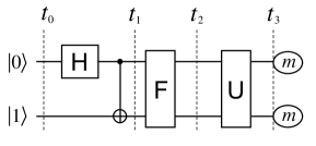
Figure 2: Quantum circuit; the gates are described in the text.

where $\mathsf{H}$ is the Hadamard gate, $\mathsf{F}$ is the $2$ qubits quantum Fourier transform, $\mathsf{U}$ is defined by

$${\mathsf{U}}:\left\{\begin{array}[]{lc}|00\rangle\mapsto|00\rangle\\ |01\rangle\mapsto\left(|01\rangle+\sqrt{2}|10\rangle+|11\rangle\right)/2\\ |10\rangle\mapsto\left(|01\rangle-\sqrt{2}|10\rangle+|11\rangle\right)/2\\ |11\rangle\mapsto\left(|01\rangle-|11\rangle\right)/\sqrt{2}\end{array}\right.$$ (24)

and the last measurements are made in the $0-1$ basis. A trivial consistent extension of this family would consist of a measurement that distinguishes the four Bell states

$$\begin{array}[]{ll}|\Phi^{\pm}\rangle=\frac{1}{\sqrt{2}}(|00\rangle\pm|11\rangle)\\ |\Psi^{\pm}\rangle=\frac{1}{\sqrt{2}}(|01\rangle\pm|10\rangle)\end{array}$$ (25)

at time $t_{1}$. This would obviously leave the final result unchanged because at time $t_{1}$ the system is in the state $|\Psi^{+}\rangle$. This measurement does not contribute to the classicality of the circuit because it is not local so the quantum information could not be substituted by classical information: entangled states cannot be represented on classical spins.

A nontrivial local consistent extension is given by measuring both qubits in the computational basis at time $t_{2}$ (this defines $\sigma^{(2)}$). To convince oneself, one should consider the graph of fig.3 constructed from the family ${\mathcal{S}}=\{|01\rangle\langle 01|,\sigma^{(1)},\sigma^{(2)},\sigma^{(3)}\}$ where we have kept the Bell measurement $\sigma^{(1)}$ for sake of analysis (if ${\mathcal{S}}$ is consistent with $\sigma^{(1)}$, it is also without since this is coarse graining).

Figure 3: Graph analysis of the quantum circuit of fig.2. The products of the Green functions around the loops are imaginary; hence, ${\mathcal{S}}=\{|0\rangle\langle 0|,\sigma^{(1)},\sigma^{(2)},\sigma^{(3)}\}$ is consistent.

Also for sake of clarity, we have indicated only the Green functions that are connected in some way to $|\phi^{(0)}_{2}\rangle=|01\rangle$ since they are the only ones that might cause problems. There are two loops in this graph, but the product of the Green functions around these loops is imaginary. Indeed, all the Green functions are real except $G_{11}(t_{2},t_{1})=\frac{-1+i}{\sqrt{8}}$ and $G_{13}(t_{2},t_{1})=\frac{-1-i}{\sqrt{8}}$ which are indicated by double lines on the graph; furthermore, $G_{11}(t_{2},t_{1})G_{13}(t_{2},t_{1})^{*}=\frac{-i}{4}$; hence the measurement $\sigma^{(2)}$ is a weakly consistent extension.

To understand what is going on, it is convenient to write the state of the system at time $t_{2}$: $|\psi(t_{2})\rangle=[2|00\rangle+(-1+i)|01\rangle+(-1-i)|11\rangle]/\sqrt{8}$. This state has 0.4165 $ebits$ of entanglement that are destroyed by the measurement $\sigma^{(2)}$. Hence, this demonstrates that it is possible to destroy entanglement in a quantum computer without affecting the final result. One could argue that the final measurement will destroy entanglement so $\sigma^{(2)}$ is only doing what would later be done by $\sigma^{(3)}$. This is the case of the semiclassical quantum Fourier transform of Griffiths and Niu GN1996 , where the final measurements were performed ahead of time, thus allowing the substitution of QIP by CIP. This is not the case here. To convince oneself, apply $\mathsf{U}^{-1}$ to the states of the final measurement—the computational states—and verify that the result is entangled. Therefore, in both directions of time, we are destroying entanglement without affecting the final result.

The skeptics can be convinced that the measurement is indeed consistent by verifying that the probability sum rules are satisfied. [Recall that the weak consistency condition that was verified with the help of the graph of fig.3 is stronger than the computing consistency condition eq.(9) which itself implies the validity of the classical probability sum rules eq.(11).] To do this, construct the transition probability matrix ${\mathcal{T}}=(t_{ij})$ where $t_{ij}$ is the probability that the system is measured in state $i$ at time $t_{3}$ after it is observed in state $j$ at time $t_{2}$ as in eq.(11). Obviously, $t_{ij}=|u_{ij}|^{2}$, the square norm of elements of matrix $\mathsf{U}$ of eq.(24). If $P_{i}(t_{k})$ denotes the probability of observing the system in state $i$ at time $t_{k}$ [i.e., $P_{i}(t_{k})=|\langle i|\psi(t_{k})\rangle|^{2}$ ], the probability sum rules should read $P_{i}(t_{4})=\sum_{j}t_{ij}P_{j}(t_{3})$. Indeed, we get

$$\left(\begin{array}[]{c}1/2\\ 3/16\\ 1/8\\ 3/16\end{array}\right)=\left(\begin{array}[]{cccc}1&0&0&0\\ 0&1/4&1/4&1/2\\ 0&1/2&1/2&0\\ 0&1/4&1/4&1/2\end{array}\right)\left(\begin{array}[]{c}1/2\\ 1/4\\ 0\\ 1/4\end{array}\right)$$ (26)

as claimed. Therefore, the effect of gate $U$ as seen from the final measurement can be simulated by a stochastic classical model.

IV.1 Classically controlled operations

At first sight, forcing the state of the computer to be classical at time $t_{2}$ might not seem so exciting. Nevertheless, Dowker and Kent have shown that if a measurement $\sigma$ appears twice in a consistent family, say at times $t_{a}$ and $t_{b}$ with $t_{a}<t_{b}$, then it can be repeated anywhere between $t_{a}$ and $t_{b}$ DK1996 . Let me translate this result in terms of quantum computing: If qubit $k$ ($q_{k}$) can be made classical at time $t_{a}$ and all operations between $t_{a}$ and $t_{b}$ are diagonal in the consistent basis of $q_{k}$, then all quantum operations between $t_{a}$ and $t_{b}$ can be replaced by classically controlled operations. This is the generalization of the observation by Griffiths and Niu GN1996 that measuring a control qubit at the end of the computation is equivalent to measuring it before the controlled operations.

IV.2 Noise robustness

The classicality analysis can be used to enhance the noise robustness of a computer for a given algorithm. Assume that $q_{k}$ can consistently be measured at time $t_{j}$. Obviously, performing this measurement would protect it against decoherence (uncontrolled measurement by an exterior environment) since its information could be encoded classically. Unfortunately, projective measurements cannot be performed in a NMR setting EBW1994 . Nevertheless, if the decoherence is in a known local basis, there is still hope. One can apply a rotation on $q_{k}$ so that the consistent basis agrees with the decoherence basis (rotating $q_{k}$ is like changing the basis in which decoherence occurs). Hence, decoherence will perturb the state of the computer but in a consistent way. This procedure can be seen as bringing the information of the quantum computer into a decoherence free-subspace; its purpose is to protect not the state but the outcome of the computation. For example, if known local decoherence takes place between gates $\mathsf{F}$ and $\mathsf{U}$ of fig.2, rotating both qubits will protect the output of the computation, no matter what state the computer is in at that time.

Now assume that the decoherence at time $t_{2}$ is still local but in an unknown basis. Entanglement will then be destroyed in an uncontrolled fashion and the refocusing scheme is of no help. Intuition tells us that the damage should be less if we first destroy the entanglement in a consistent fashion and then let decoherence perturb the system. In other words, before local decoherence takes place, we force the system into a local state, hoping to reduce its effect. (This is like preventing forest fires by burning them down!) This intuition can be verified using our toy model of fig.2. Decoherence will result in a probability distribution $\tilde{P}$ over the final outcomes that is different from the original unperturbed distribution $P$. The error due to decoherence can be measured by the relative entropy $H(P||\tilde{P})$ (Kullback-Leibler distance CT1991 ). This entropy is calculated in two situations: $H_{0}$ measures the error caused by decoherence in the absence of the consistent measurement at time $t_{2}$; $H_{m}$ is the error due to decoherence when the system is forced into local state at time $t_{2}$. Since the local basis in which decoherence occurs is unknown, we must average the entropies over all local bases—integrate over two Bloch sphere surfaces—we obtain a reduction of relative entropy of about $25\%$ when consistent measurements are applied. (A statistician’s $\chi^{2}$ approach gives very similar results.)

IV.3 Mixed states

Whether mixed state quantum computing can increase one’s computational power over classical computing is a question of great interest. The main objection to such an increase is that, when the state is highly mixed, it can always be written as a mixture of unentangled states. Hence, it is possible that a mixed state algorithm can be decomposed into a mixture of pure state algorithms that are in local states throughout the computation PP2001 . This would suggest that the mixed state algorithm can be simulated efficiently by a classical probabilistic computer. On the other hand, recent work by Knill and Laflamme KL1998 gives indications that the answer is positive, but does not provide a proof.

When the initial state of the quantum computer is pure, the absence of entanglement throughout the computation implies that all gates in the circuit are classical and therefore can trivially be simulated on a classical device BCJLPS1999 . When the initial state is highly mixed, even fundamentally quantum operations will not create entanglement. At first sight, this seems to imply that these systems behave classically. Here, I show that, while the state of the quantum computer is stroboscopically classical, no classical dynamics can logically explain its evolution.

Consider a state of the the form eq.(23). For a two-event family, the coherence function eq.(4) reads

$$Tr\left\{P^{(2)}_{\alpha_{2}}P^{(1)}_{\alpha_{1}}\rho P^{(1)}_{\beta_{1}}P^{(2)}_{\beta_{2}}\right\}$$

$$= \frac{(1-\nu)}{\Omega}\delta_{\alpha_{1}\beta_{1}}\delta_{\alpha_{2}\beta_{2}}Tr\left\{P^{(2)}_{\alpha_{2}}P^{(1)}_{\alpha_{1}}\right\}$$

$$+ \nu\delta_{\alpha_{2}\beta_{2}}Tr\left\{P^{(2)}_{\alpha_{2}}P^{(1)}_{\alpha_{1}}|\psi\rangle\langle\psi|P^{(1)}_{\beta_{1}}\right\}$$

so the family is consistent if and only if the family with initial pure state $|\psi\rangle$ is consistent. To complete the argument, choose your favorite two-event family whose evolution cannot be explained in a local fashion when the initial state is pure (I suggest Young’s slit experiment). This does not answer the question concerning the computational power of mixed states but it indicates that there is something fundamentally quantum in their evolution, so the main objection does not hold.

In fact, one can build a strong intuition about this result using Young’s slit experiment. Assume that the experiment is performed using a “pseudocoherent” light source. For example, one could point a laser and a regular (incoherent) light at the slits both at the same time. Without the regular light, one observes the usual interference pattern. This implies that most photons from the laser go through both slits. When the regular light is added, the observed pattern is the classical superposition of a smooth pattern (no interference) and the original interference pattern. This cannot be explained without admitting that some photons still go through both slits. Hence, even if a great number of photons are not in a coherent phase, some fundamentally quantum phenomenon is still taking place.

IV.4 Uniformity

When analyzing a quantum circuit, one should be concerned with the notion of uniformity. A quantum algorithm is represented by a family of quantum circuits, one for each input size. The construction rule for circuit of size $\ell+1$ given the one of size $\ell$ must be simple. Therefore, a consistency analysis should be uniform, otherwise it is useless in practice. The semiclassical quantum Fourier transform of Griffiths and Niu is an example of a uniform consistency analysis.

From this point of view, the analysis of the circuit shown in figure 2 is not quite illuminating since it does not belong to a family of circuits. Nevertheless, this example was not intended as a practical one, but was used to illustrate a crucial point: the dynamics generated by gate $\mathsf{U}$ on state $|\psi(t_{2})\rangle$, while highly nonclassical for the reasons mentioned earlier, is classical as seen from the measurements. In other words, there are fundamentally quantum effects happening in the circuit, but the fixed final measurement is blind to this quantumness. This would be impossible if we required the extensions to be consistent for all choices of final measurement; fortunately, the final measurements are fixed in a quantum circuit.

The notion of uniformity allows us to weaken the locality restriction on the sets of projectors. By restraining the measurement to single qubit, we can simulate the effective dynamics of the quantum system by classical spins, or equivalently by keeping track of two angles and a radius of a Bloch sphere vector per qubit. By going to higher dimensional classical simulators, we can perform joint measurements on many qubits. Nevertheless, in order to have the size of the classical simulator growing polynomially, one should restrict the size of these joint measurements to be logarithmic. Here the notion of uniformity is crucial.

This is a generalization of the result of Aharonov and Ben-Or AB1996 mentioned in the introduction. They established that the absence of large scale coherence in a quantum system allows an efficient classical simulation. Here I show that it is not the absence of coherence that is crucial but the absence of effective coherence—the one that affects the coherence function.

V Conclusion

I have shown that not all the information processed by a quantum computer is required to be quantum for the success of the algorithm. The CH formalism together with an extra condition indicates how and when one can substitute quantum information by classical information. Classicality has helped increase the noise robustness of a quantum computer. It has also given new indications on the controversial question of computing with mixed states.

Quantum systems seem to be hard to simulate classically. Feynman’s argument—the exponentially growing size of the matrices—misses an important point: only a linear fraction of this information is accessible by fixed measurement. To be fair, classical simulation of quantum systems should be concerned only with effective dynamics—the dynamics seen by the measurements. The CH formalism is the appropriate tool to describe this dynamics.

Classicality also allows the use of different implementations of quantum computers within the same computation. Since the information conveyed by the computer is made classical at different stages of the computation, it can easily be transferred to a different system. This new possibility might also have implications in multiparty quantum computing.

The most exciting feature of classicality is that a complete CH analysis of an algorithm would pinpoint what is fundamentally quantum in it, hence answering the question “What gives the extra computing power to quantum mechanics, if any?” Unfortunately, a complete analysis is at this time impossible since the right tools have not been found. The results of section 3 and DK1996 provide new hints in this direction but further studies are required. It is encouraging to notice that what is probably the most promising tool—feedback—has not even been explored up to now.

References

- (1) Bernstein E. and Vazirani U., Proc. 25th Annual ACM Symp. on Theory of Comp., ACM, 11 (1993).
- (2) Simon D.R., IEEE FOCS’94, 116 (1994).
- (3) Shor P.W., IEEE FOCS’94, 124 (1994); Shor P.W., SIAM J. comput. 26 1484 (1997).
- (4) Żurek W.H., Phys. Today October 1991, 36; Landauer R., Phil. Trans. Roy. Soc. of London 853 367, (1995); Unruh W.G., Phys. Rev. A 51 992 (1995).
- (5) Aharonov D. and Ben-Or M., Proc. of the 29th Annual ACM Symposium on Theory of Computing, (1997); Kitaev A.Y., Uspekhi Mat. Nauk. 52 53 (1997); Preskill J., Proc. Roy. Soc. of London A 454 385 (1998).
- (6) Knill E., Laflamme, R. and Żurek W.H., Science 279 342 (1998).
- (7) Shor P.W., Phys. Rev. A 52 2493 (1995); Knill E. and Laflamme R., Phys. Rev. A 55 900 (1997); Steane A.M., Phys. Rev. Lett. 77 793 (1996).
- (8) Gottesman D., Phys. Rev. A 54 1862 (1996).
- (9) Shor P.W., IEEE FOCS’96, 56 (1996).
- (10) Feynman R.P., Int. J. Theoretical Phys. 21 467 (1982)
- (11) Aharonov D. and Ben-Or M., IEEE FOCS’96, 46 (1996).
- (12) Żurek W.H., Phys. Rev. D 24 1516 (1981).
- (13) Bernstein E. and Vazirani U., SIAM J comput. 26 1411 (1997).
- (14) Cleve R. and Watrous J., IEEE FOCS’00, 526 (2000).
- (15) Griffiths R.B., J. Stat. Phys. 36 219 (1984).
- (16) Omnès R., J Stat. Phys. 53 893 (1988); Rev. Mod. Phys. 64 339 (1992).
- (17) Gell-Mann M. and Hartle J.B., in Complexity, Entropy and the Physics of Information, Santa Fe Institute Studies in the Science of Complexity, Vol VIII, ed. Żurek W H, 425 (1990).
- (18) Gell-Mann M. and Hartle J.B., in Physical Origins of Time Asymmetry, ed. Halliwell, J.J. and Pérez-Mercader, J. and Żurek, W.H., 311 (1994).
- (19) Gell-Mann M and Hartle J.B., lanl e-print gr-qc/9509054 (1995).
- (20) Gell-Mann M. and Hartle J.B., Phys. Rev. D 47 3345 (1993).
- (21) Dowker F. and Kent A., J Stat. Phys. 82 1575 (1996).
- (22) Paz J.P. and Żurek W.H., Phys. Rev. D 48 2728 (1993).
- (23) Diósi L., Phys. Lett. A 203 267 (1995).
- (24) Everett H. III, Rev. Mod. Phys. 29 454 (1957).
- (25) Griffiths R.B., Phys. Rev. Lett. 70 2201 (1993).
- (26) Cory D.G., Fahmy A.F. and Havel T., Proc. Natl Acad. Sci. USA, 94 1634 (1997).
- (27) For a survey, see Cory D.G, et al., lanl e-print quant-ph/0004104 (2000).
- (28) Griffiths R.B. and Niu C.-S., Phys. Rev. Lett. 76 3228 (1996).
- (29) Ernst R.R, Bodenhausen G. and Wokaun A., Principles of Nuclear Magnetic Resonance in One and Two Dimensions, Oxford University Press, Oxford (1994).
- (30) Cover T.M., Thomas J.A., Elements of Information Theory, John Wiley & Sons, (1991).
- (31) Knill E. and Laflamme R., Phys. Rev. Lett. 81 5672 (1998).
- (32) Jozsa R. cited in Parker S. and Plenio M.B., lanl e-print quant-ph/0102136 (2001).
- (33) Braunstein S.L., Caves C.M., Jozsa R., Linden N., Popescu S. and Schack R. Phys. Rev. Lett 83 1054 (1999).