Entropy production due to coupling to a heat bath in the kicked rotor problem

Abstract

Considering a kicked rotor coupled to a model heat bath both the classical and quantum entropy productions are calculated exactly. Starting with an initial wave packet, the von Neuman entropy as a function of time is determined from the reduced density matrix while the Liouville evolution of the corresponding Husimi distribution provides us with the classical entropy. It is found that both these entropies agree reasonably satisfying the same asymptotic growth law and more importantly both are proportional to the classical Liapounov exponent.

PACS numbers:03.65.Bz,05.40.+j,05.45.+b keywords: quantum open system, entropy

The question of quantum classical correspondence in the context of open systems is an interesting one. It has been argued, for instance by Zurek and Paz[1], that even a weak interaction with a random environment leads to the loss of quantum coherence and that classical behaviour may then be an emergent property of such systems. In other words, environmental effects may have a significant role to play in quantum classical correspondence in general and in the quantum dynamics of classically chaotic systems in particular. The von Neumann entropy production of an unstable oscillator interacting with a heat bath has been shown [1] to depend monotonically on the classical local Lyapunov exponent. A more extensive study of the kicked rotor in a bath by Miller and Sarkar [2] brings out in greater detail this correspondence between quantum entropy production and classical Lyapunov exponent. The quantum evolution of classically chaotic open systems has been shown to possess a sensitive dependence on initial conditions [3] and provides another interesting indication of the role of the environment. As a further instance one may mention the high degree of sensitivity of quantum dynamic localization [4] to the presence of noise found in a study on the kicked rotor [5].Extensive studies of the kicked rotor coupled to a bath were carried out by Dittrich and Graham[6] and by Cohen[7]. These authors were interested in reducing the problem and showing its equivalence to a classical stochastic map in the semiclassical limit with the aid of the Wigner function representation of the density matrix.

In the present paper we look into a few aspects of quantum classical correspondence in open systems by focussing on the kicked rotor interacting with a bath of harmonic oscillators through what is termed a nondemolition coupling. The latter involves an interaction Hamiltonian commuting with the system Hamiltonian as a result of which the reduced density matrix can be obtained exactly [8]. This feature has been used in [2] in computing the von Neumann entropy production rate of the kicked rotor. We show that the special nature of the coupling allows one to obtain the classical reduced distribution function [9] as well and then to compare the diffusion rate and the entropy production at the classical and quantum levels under similar initial conditions. Numerical computations show that in the semiclassical limit the asymptotic von Neuman entropy follows the same classical growth law as obtains for a diffusion process viz. $s(t)=A+B\ln t$ and that this regime is established smoothly after a very few kicks even for relatively weak bath couplings. Of more interest is the fact that in the asymptotic region the quantum entropy is proportional to the classical Liapounov exponent which may perhaps be looked upon as a signature of quantum chaos in semiclassical quantum mechanics.

We take a cylindrical phase space ($0<q\leq 2\pi;-\infty<p<\infty$) and define the kicked rotor Hamiltonian to be,

$$H_{rotor}=p^{2}/2+K\cos q\sum_{n=-\infty}^{+\infty}\delta(t-n).$$ (1)

The classical dynamics is defined by the standard map,

$$p_{n+1} = p_{n}+K\sin q_{n+1},$$ (2)

$$q_{n+1} = q_{n}+p_{n}\;\;\;\;\;\;\;\;\;mod\>2\pi,$$ (3)

where $q_{n}$ and $p_{n}$ are the values just after the $n$th kick. Below a critical kick strength $K_{c}(\sim.97)$ KAM tori prevent the indefinite growth in energy while above $K_{c}$, one has a mixed phase space of islands surrounded by a chaotic sea and the diffusive growth law holds viz. $\langle(p_{n}-p_{0})^{2}\rangle=D(K)n,$ where the average is over a distribution of initial points and the diffusion coefficient tends to $K^{2}/2$ for large $K$. In quantum mechanics the evolution is governed by the single step unitary evolution operator which takes the state from just after the $n$th kick to just after the $(n+1)$th kick and is given by,

$$U(n+1,n)\equiv U_{k}U_{f}=\exp[{iK\over\hbar}\cos q]\exp[-ip^{2}/(2\hbar)].$$ (4)

In the momentum representation $U_{f}$ is just a phase factor and the matrix element for $U_{k}$ is given by,

$$\langle l\mid U_{k}\mid m\rangle=(i)^{l-m}J_{l-m}(K/\hbar).$$ (5)

Numerical computation with an initial wave packet shows a diffusive growth in energy for a finite time determined by the values of $K$ and $\hbar$ after which the energy oscillates quasiperiodically about an average value [4, 10].

The total Hamiltonian for a system with a nondemolition coupling to an oscillator bath is chosen to be,

$$H = H_{0}(p)+{1\over 2}\sum_{k}(p_{k}^{2}+\omega_{k}^{2}q_{k}^{2})$$ (6)

$$+\phi(H_{0})\sum_{k}c_{k}\sqrt{\omega_{k}}q_{k}+{1\over 2}\sum_{k}{c_{k}^{2}\over\omega_{k}}\phi^{2}(H_{0}),$$

where the first two terms are the system and bath Hamiltonians respectively. The third term is the interaction with $c_{k}$ being the coupling constant to the $k$th mode, $\phi$ being an arbitrarily chosen function, while the fourth one is a renormalization term. We will work out the time evolution for a general Hamiltonian $H_{0}(p)$ and then specialize to the case of the rotor. Notice that the interaction is a function of the system Hamiltonian and therefore momentum will be conserved. Making a canonical transformation with the generating function,

$$F(q,q_{k};P,P_{k})=qP+\sum_{k}q_{k}P_{k}+\phi(P)\sum_{k}{c_{k}\over\omega_{k}^{3/2}}P_{k},$$ (7)

the Hamiltonian is reduced to the uncoupled form,

$$H=H_{0}(P)+{1\over 2}\sum_{k}(P_{k}^{2}+\omega_{k}^{2}Q_{k}^{2}).$$ (8)

Solving the equations of motion obtained from  (8) and reverting back to original variables we get our required solutions viz. $q(0)\text{ and }p(0)$ in terms of $q,p,q_{k}(0)\text{ and }p_{k}(0)$. As an initial point $\{q(0),p(0)\}$ evolves in time $t$ to $\{q,p\}$ the distribution function evolves from $f^{0}[q(0),p(0)]$ to $f[q,p]$ maintaining its value at the corresponding points. However, since the evolution depends on the bath variables, the reduced distribution function is obtained by integrating over the bath quantities which are assumed initially to have values pertaining to thermal equilibrium. Thus,

$$f_{red.}(q,p,t)=\int f^{0}[q(0),p(0)]\prod_{k}{g_{k}\over z_{k}}dp_{k}(0)dq_{k}(0),$$ (9)

where in the r.h.s. $[q(0),p(0)]$ are understood to be written in terms of $[q,p]$. The factor $g_{k}$ is the thermal probability for the $k$th bath mode at temperature $T(=1/\beta)$ and it is normalized by the partition function $z_{k}$. We carry out the integration in equation (9) and go to the continuum limit whereby the sum over modes is replaced by an integration over frequency with an ohmic spectral density function given by,

$$\sum_{k}\rightarrow\int f(\omega)d\omega,~{}~{}~{}~{}f(\omega)=\eta{\omega\over c^{2}(\omega)}e^{-{\omega/\omega_{c}}}.$$ (10)

The reduced distribution function is given by,

$$f_{red.}(q,p,t) = \sqrt{\frac{\beta}{2\pi s(t)}}\int drf^{0}[q-({\partial H_{0}\over\partial p})t+r$$ (11)

$$-\phi\phi^{\prime}\eta\arctan\omega_{c}t,p]\exp(-\frac{\beta r^{2}}{2s(t)}),$$

$$s(t) = 2\eta{\phi^{\prime}}^{2}[t\arctan\omega_{c}t-\frac{1}{2\omega_{c}}\ln(1+\omega_{c}^{2}t^{2})].$$ (12)

If we look at the fundamental solution of  (11) when $f^{0}$ is a $\delta$-function we find $f_{red.}$ to be a gaussian . For $\omega_{c}t\ll 1,$ $s(t)\propto t^{2}$ and the gaussian spreads fast but after some time depending on $\omega_{c}$, $\arctan\omega_{c}t$ saturates at $\pi/2$ and $s(t)\propto t$, so that equation (11) describes a normal diffusion process. In the case of the rotor $(\partial H_{0}(p)/\partial p)=p$, and for the coupling we take $\phi(p)=p$, so that $\phi^{\prime}=1$. The fourth term in (6) therefore renormalizes the rotor mass. Because of the nondemolition nature of the coupling the $p$-distribution remains the same in the absence of the kicking term whereas the $q$-distribution suffers a shift and a gaussian local averaging. However, as it turns out, the bath brings about a mixing in the $p$-distribution on a fine scale when the kicks couple $q$ and $p$. .

For the quantized form of the Hamiltonian (6) the matrix elements of the reduced density operator for the rotor at time $t$ are given by [2, 8],

$$\langle m\mid\rho_{red.}(t)\mid n\rangle = \exp[-i\hbar(m^{2}-n^{2})t/2]$$ (13)

$$\langle m\mid\rho(0)\mid n\rangle\>\exp[-iA^{1}_{mn}-A^{2}_{mn}],$$

where,

$$A^{1}_{mn} = \eta\hbar(m^{2}-n^{2})\tan^{-1}\omega_{c}t,$$ (14)

$$A^{2}_{mn} = {\eta\hbar\over 2}(m-n)^{2}\ln(1+\omega_{c}^{2}t^{2})$$ (15)

$$+\eta\hbar(m-n)^{2}\ln\prod_{k=1}^{\infty}\{1+({\omega_{c}t\over 1+k\beta\omega_{c}})^{2}\}.$$

Notice that the diagonal matrix elements are unaffected by the interaction with the bath when the kicking term is absent.

In analysing the quantum evolution we take an initial normalized wave packet of the form, $\mid\psi\rangle=\sum_{l}a_{l}\mid l\rangle$ which is localized and peaked around the momentum $p=\hbar l_{0}$. We achieve similar initial conditions for the classical evolution by taking the Husimi distribution [11] corresponding to $\mid\psi\rangle$. This is given by,

$$f(q,p)\equiv\mid\langle q,p\mid\psi\rangle\mid^{2} = \sum_{m,n}{a_{m}^{*}a_{n}\over\sqrt{\pi}}\exp[-p^{2}/\hbar^{2}$$

$$+(m+n)p/\hbar - (m^{2}+n^{2})/2]\cos(m-n)q,$$ (16)

which is a diagonal approximation of the density matrix in the coherent state representation. $f(q,p)$ is periodic in $q$ with period $2\pi$ so that (16) is really defined on the cylinder. The coefficients $a_{l}$ are chosen such that $\mid\psi\rangle$ represents a wave packet with $\Delta p=\Delta q=\hbar/2$. This is achieved by parametrising $a_{l}$ in the form, $a_{l}=N\exp[-al^{2}+bl],$ where $a$ is real and $b$ is complex such that the three parameters $a$ and the real and imaginary parts of $b$ determine the centre and the width of the wave packet.

For the quantum evolution the computation starts with the density matrix corresponding to $\mid\psi\rangle$. After unit time step the reduced density matrix is evaluated using equation (13). The unitary kick operator $U_{k}$ then connects the matrix elements for the density operators just before and after the kick according to (4). The von Neumann entropy is calculated by using the definition,

$$S\equiv-Tr\rho\ln\rho=-\sum_{i}\lambda_{i}\ln\lambda_{i},$$ (17)

where the $\lambda_{i}$ are the eigenvalues of the density operator. The computation is repeated till the entropy reaches its asymptotic growth rate. To compute the classical evolution we start with the Husimi distribution corresponding to the initial quantum wave packet and use equation (9) to find the reduced distribution after unit time step. The distributions just before and after the kicks are related by a simple shift in argument viz. $f_{red.}^{+}(q,p)=f_{red.}^{-}(q,p-K\sin q).$ The entropy is calculated by using the formula,

$$S_{H}=-\int f\ln f{dpdq\over 2\pi\hbar},~{}~{}~{}~{}~{}~{}~{}~{}~{}~{}~{}~{}\int f{dpdq\over 2\pi\hbar}=1.$$ (18)

It is known that $S_{H}$ calculated from $f(q,p)$ as defined in (16) satisfies the inequality, $S_{H}\geq S.$ It turns out that the classical approximation is good as long as $f(q,p)$ is a smooth function spread over an area in phase space that is much greater than $2\pi\hbar$. If there are small distance fluctuations or if $f(q,p)$ is concentrated on a small region of the phase space, then the classical approximation can be very bad [9]. This fact will be borne out in our numerical computations. Notice that the von Neumann entropy for the initial pure state is zero. However, this is not true of (18). The Husimi distribution corresponding to the initial wave packet is sufficiently well localised in $q$ to be considered a gaussian with $\Delta p\Delta q=\hbar$ and its entropy is just unity.The distribution is chosen to be centred at $q=0,p=\pi\hbar$ which lies in a chaotic region for all the $K$-values cosidered by us.

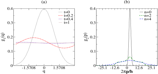
Figure 1: Evolution of (a) $g_{1}(q)$ and (b) $g_{2}(p)$ for $\eta=1.0,K=3.5$.

To understand the diffusion process in detail we compute the $q$-distribution, $g_{1}(q)$ and the $p$-distribution, $g_{2}(p)$ as the integrals of $f(q,p)$ over $p$ and $q$ respectively. The diffusion rate in $q$ is controlled by the parameter $\omega_{c}$ and $\beta$. For our choice, $\omega_{c}=5/\hbar\approx 10\text{ and }\beta=0.1$ satisfying $\beta\hbar\omega_{c}<1$, we find that $g_{1}(q)$ almost reaches the value $({1\over 2\pi})$ before the first kick [fig. (1a)]. Decreasing $\omega_{c}$, will increase the equilibriation time for the $q$-distribution. The large scale structure of the $p$-distribution on the other hand is determined by the kicks, the bath providing a mixing on a finer scale through the coupling with the kicks. Figure (1b) shows the initial evolution of $g_{2}(p)$.

Next, we compute the classical and quantum energies. The effect of $\hbar$ for fixed $K$ (the relevant parameter actually is $K/\hbar$) on the variation of $\langle E\rangle$ with $t$ as also on the entropy production (see below; neither of these two is shown in our figures) indicates that one can distinguish between a semiclassical and strongly quantum regime: while oscillations due to quantum correlations are pronounced in the latter, they are almost absent in the former. All our numerical work relates mainly to the semiclassical regime with $\hbar$ taken as a rational multiple of the golden mean $(\sqrt{5}-1)/2$ to avoid resonances. The energy growth is typically diffusive for both classical and quantum dynamics and the diffusion rate increases with $K$. What is interesting is the effect of the bath coupling strength $\eta$ on the energy growth (fig.2): on increasing $\eta$ from a low value one finds that the classical and quantum energy growth curves quickly approach each other (cf. Ott, Antonsen and Hanson [5]) and their growth rates saturate at $K^{2}/4$ even for comparatively low values of $K$. This is consistent with the role of the bath outlined above.

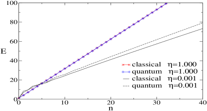
Figure 2: Comparison of classical and quantum energy growth for $K=3.5,\hbar=0.46$.

Figures (3(a,b)) present results on entropy production. Note that there is an $\hbar$ dependence in the classical entropy $S_{H}$ arising from the Husimi density corresponding to an initial wave packet. The evolution of the Husimi density satisfies the Liuville equation in the lowest order in $\hbar$ and that is what we have considered here. The classical and quantum entropy productions are compared in fig. 3(a) which shows that the two converges quickly excepting for comparatively large values of $\hbar$ and even when they differ their asymptotic growth rates agree. The time dependence of entropy production is elucidated in fig. 3(b) which uses a logarithmic time scale: asymptotically the entropy settles down to a logarithmic growth. Curves for different values of $\eta$ once again show a quick saturation with increasing $\eta$.

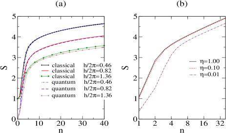
Figure 3: Entropy growth in the quantum case for (a) different $\hbar$ with $K=3.5,\eta=10^{-2}$ and (b) different $\eta$ with $K=3.5,\hbar=0.46$.

The asymptotic entropy production fits nicely with the formula $S=A+B\ln n$ which we now explain by referring to the classical entropy $S_{H}$. Entropy production occurs due to the coarse graining provided by the bath along with the diffusion provided by the kicks. The bath quickly uniformizes the q-distribution and converts the p-distribution to a smoothed gaussian so that in the asymptotic regime

$$f(q,p)={\hbar\over{\sqrt{2\pi}\Delta p}}exp{(-{p^{2}\over{2\Delta p^{2}}})}.$$

Together with the diffusive growth law, $\Delta p=(K/\surd 2)n^{1\over 2}$ this yields for the entropy,

$$S_{H}={1\over 2}+\ln({\sqrt{\pi}\over\hbar})+\ln K+{1\over 2}\ln n.$$ (19)

Since for large $K$, the Lyapunov exponent is, $\lambda=\ln{K\over 2}$, the coefficient $A$ is linear in the Lyapunov exponent for large $K$.

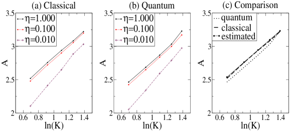
Figure 4: Variation of $A$ with $\ln K$ for different $\eta$ in the (a) classical and (b) quantum case. (c) shows a comparison with the values estimated from (19) for $\eta=1.0$.

The growth law $S=A+B\ln n$ with $A$ depending linearly on $\ln K$ and $B=1/2$ is numerically found to apply to the quantum entropy as well in the semiclassical regime. Figures 4(a,b) depicts the variation of $A$ with $\ln K$ as computed numerically from the classical and quantum entropy production data where the linear dependence is evident and where the role of $\eta$ in quantum classical correspondence is apparent once again. Figure 4(c) compares the numerically computed values of $A$ with the estimated values from equation (19).

Figures 5(a,b) present corresponding data for the coefficient $B$ which is indeed found to be close to $1/2$. The discrepancy is explained by the presence of residual phase space barriers to diffusion as also incomplete mixing which disappears more and more with increasing $K$ and $\eta$. In figures 4 and 5, $\hbar$ is held at $0.46$.

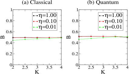
Figure 5: Plot of $B$ with $K$ for different $\eta$ in (a)classical case and (b)quantum case.

In conclusion, the findings presented above underline the role of the bath in establishing a quantum-classical correspondence wherein the quantum entropy production carries with it the characteristics of the classical phase space structure: for instance, the quantum entropy is tied to the classical Lyapunov exponent [1, 2]. It would be interesting to look into the entropy production in the kicked Harper model where the phase space is compact and the diffusive growth law $(\Delta p\propto\sqrt{n})$ does not hold.

References

- [1] W. H. Zurek and J. P. Paz, Phys. Rev. Lett.72, 2508 (1994); see however, G. Casati and B.V. Chirikov, Phys. Rev. Lett.75, 350 (1995) for an alternate view on the role of external noise.
- [2] P. A. Miller and S. Sarkar, Nonlinearity 12, 419 (1999).
- [3] M. Toda,S. Adachi and K. Ikeda, Prog. Theo. Phys. Suppl. 98, 323 (1989).
- [4] G. Casati, B. V. Chirikov, J. Ford and F. M. Izrailev, Lecture Notes in Physics 93, 334 (1979).
- [5] E. Ott, T. M. Antonsen, Jr. and J. D. Hanson, Phys. Rev. Lett. 53, 2187 (1984).
- [6] T. Dittrich and R. Graham, Ann. Phys. 200 (1990) 363.
- [7] D. Cohen, J. Phys. A 27 (1994) 4805 and references contained therein.
- [8] J. Shao, M. Ge and H. Cheng, Phys. Rev. E 53, 1243 (1996).
- [9] A. Wehrl, Rev. Mod. Phys. 50, 221 (1978).
- [10] F. M. Izrailev, Phys. Rep. 196, 300 (1990).
- [11] K. Takahashi, Prog. Theo. Phys. Suppl. 98, 109 (1999).