Exploring Hilbert Space: accurate characterisation of quantum information

Abstract

We report the creation of a wide range of quantum states with controllable degrees of entanglement and entropy using an optical two-qubit source based on spontaneous parametric downconversion. The states are characterised using measures of entanglement and entropy determined from tomographically determined density matrices. The Tangle-Entropy plane is introduced as a graphical representation of these states, and the theoretic upper bound for the maximum amount of entanglement possible for a given entropy is presented. Such a combination of general quantum state creation and accurate characterisation is an essential prerequisite for quantum device development.

Quantum information (QI) - the application of quantum mechanics to problems in information science such as computation and communication - has led to a renewed interest in fundamental aspects of quantum mechanics. In particular much attention has been focussed on the role of entanglement, the non-classical correlation between separate quantum systems, particularly between two-level systems or qubits (quantum bits). Entanglement, along with the degree of order, or purity, determines the utility of a given system for realising various QI protocols. A key goal of QI is the experimental realisation of complex quantum algorithms, e.g., Shor’s algorithm, which allows efficient factoring of composite integers [1]: recent research indicates that while entanglement is necessary to execute Shor’s algorithm, pure states are not [2].

There is currently a global effort to manufacture two-qubit gates, since any quantum algorithm can be implemented by a combination of single qubit rotations and such gates (which produce the necessary entanglement) [3]. These are fully characterised only when both the gate states and its dynamics have been accurately measured, which requires a tunable source of two-qubit quantum states and a method of completely measuring the output states [4]. No system to date has fulfilled these criteria. Here we report an optical two-qubit source that produces a wide range of quantum states with controllable degrees of purity and entanglement, and fully characterise these states by quantum tomography. This source is also suitable for exploring alternative paradigms: (1) where quantum algorithms are implemented via single qubit rotations, Bell-state measurements, and a pre-determined set of entangled states (which may or may not need to be pure) [5]; (2) scaleable linear-optics quantum computation, where entanglement occurs as a result of measurement [6].

Quantum states of N qubits can be represented by a vector existing in a $2^{\rm{N}}$-dimensional Hilbert space. This is the “space of possibilities”, and represents all possible physical combinations of qubits for a system. To date the states generated in QI experiments have clustered around two distinct limits in Hilbert space: 1) highly entangled systems with high order [7, 8, 9, 10, 11]; 2) completely unentangled systems with very little order [12]. The lack of entanglement in the latter case [13] has raised the question of what properties are actually required for quantum information protocols, and highlights that to date, the “domain of mixed states between these two extremes [pure vs. completely mixed] is incredibly big and largely unexplored.” [14]. We experimentally explore this unmapped region, and introduce a theoretical upper bound for the maximum amount of entanglement possible for a given purity. A variety of measures exist for quantifying the degrees of disorder and entanglement, all of which are functions of the system density matrix. For our experimental system, the density matrix can now be obtained via quantum tomography [15], allowing these measures to be applied. In this paper we will use the tangle, T, to quantify the degree of entanglement, and the linear entropy, $\rm{S}_{\rm{L}}$, to quantify the degree of disorder [16].

We obtain our quantum states via spontaneous downconversion, where a pump photon passed through a nonlinear crystal is converted into a pair of lower energy photons. We use the polarisation state of the single photons as our qubits, and measure in coincidence, thus obtaining the reduced density matrix (it only describes the polarisation component of the state) of the two-photon contribution [20]. Figure 1 is a schematic of the experimental system; a detailed description is given elsewhere [22]. Briefly, the BBO crystals produce pure-state pairs of photons that can be tuned between the separable and maximally entangled limits by adjusting the pump polarisation [15]. The parity and phase of the entangled states are selected via the “state selector” half-wave plates, and the photons are analysed using adjustable quarter- and half-wave plates (QWP & HWP) and polarizing beamsplitters (PBS), which enable polarisation analysis in any basis. (For tomography, 16 different coincidence bases are required [15, 23]). The photons are passed via suitable optics to single photon counters, whose outputs are recorded in coincidence.

To change the entropy it is necessary to introduce decoherence into the polarisation degree of freedom, which can be done either spatially or temporally. Decoherence can occur when the phase, $\phi$, of the entangled state (e.g. $|\rm{HH}\rangle+e^{i\phi}|\rm{VV}\rangle$) varies rapidly over a small spatial extent, i.e. smaller than the collection apertures. We achieved this by the introduction of BBO crystals (3 mm thick) into the downconversion beams, cut so that their optic axes were at an angle of $49^{\circ}$ to the beam. These introduce a highly direction-dependent phase shift in the downconverted photons: due to the intrinsic spread of photon momentum in downconversion, and the high birefringence of BBO, after the decoherer the phase of the entanglement is very finely fringed compared to the collection aperture. Figure 2a shows that with BBO in only one arm (optic axis at 45^∘), the resultant state is partially mixed and completely unentangled, ($\rm{S_{L}}$,T)=($0.66\pm 0.03$, $0.00\pm 0.00$); adding a BBO crystal to the remaining arm, (optic axis at 0^∘) generates a fully mixed state, ($\rm{S_{L}}$,T)=($1.00\pm 0.01$, $0.00\pm 0.00$).

As spatially-based decoherence completely destroys entanglement, it is not a suitable technique for exploring Hilbert space. In contrast, temporally-based polarisation decoherence allows entanglement to survive. It is achieved by imposing a large relative phase delay, longer than the coherence length of the light, between two orthogonal polarisations. In practice this is realised by introducing a 10mm thick quartz crystal in each arm, with optic axes vertical and perpendicular to the beam. The detected photons have a coherence length of  140 wavelengths (set by the 5 nm interference filters): 10 mm of quartz delays the phase velocity of the horizontally polarised light by this amount (relative to the vertical). Viewed differently, the quartz entangles the phase to the photon frequency, which is then traced over [24, 25]. Thus, a single photon linearly polarised at 45^∘ would exit the quartz crystal strongly depolarised, i.e. in a mixed state; similarly, a pair of photons, each at 45^∘, would exit two such crystals in a mixed state. With entangled states, however, the situation is more subtle. Certain kinds of entangled states are immune to collective decoherence, whilst others exhibit strong decoherence - the former comprise decoherence free subspaces [26]. Due to the energy entanglement of the photons, and the alignment of our decoherers, in our system the state $(|\rm{HH}\rangle+|\rm{VV}\rangle)/\sqrt{2}$ is decoherence free [24, 27]. The function of the state selector is to continuously tune this state towards another maximally-entangled state, one that is not decoherence-free (e.g. $(|\rm{HV}\rangle+|\rm{VH}\rangle)/\sqrt{2}$).

Figures 2b & 2c show a range of density matrices generated via this method. In Figure 2b, selector waveplate HWP1 was fixed at $0^{\circ}$ and HWP2 varied by the angle indicated; Figure 2c shows a similar series, except this time starting with a non-maximally entangled state. There are 16 parameters in the density matrix, too many for easy assimilation. To see how much of Hilbert Space we are accessing with these states, we use the tangle and linear entropy measures to construct a characteristic plane as a succinct, compact way of representing the salient features of a quantum state. In this plane (Figure 3), a pure, unentangled state lies at the origin ($\rm{S_{L}}$,T)=(0,0); a pure, maximally-entangled state in one corner ($\rm{S_{L}}$,T)=(0,1); and a maximally-mixed, unentangled state in the corner diagonally opposite ($\rm{S_{L}}$,T)=(1,0). A maximally-entangled, maximally-mixed state ($\rm{S_{L}}$,T)=(1,1) is obviously impossible. As indicated above, previous QI experiments have generated states either near the tangle axis ($\rm{S_{L}}\sim 0$, $0\leq\rm{T}\leq 1$) (cavity QED, ion and photon experiments) or at the maximally mixed point ($\rm{S_{L}}\sim 1-10^{-4}$ to $1-10^{-6}$, $\rm{T}=0$) (high-temperature NMR experiments). In Figure 3, we plot the linear entropy and tangle values determined from a range of our measured density matrices, including those shown in Figure 2 and from [28]. Two sources of experimental uncertainty were considered: statistical uncertainties ($\sqrt{N}$, where $N$ is the count), which range from 1-4% for our count rates; and settings uncertainties, due to the fact that the analysers can only be set with an accuracy of $\pm 0.25^{\circ}$. The combination of these effects led to the uncertainties as shown - a full derivation of their calculation is lengthy and given elsewhere [23]. The heavy black line in Figure 3 represents the (S,T) values of Werner states ($\hat{\rho}_{W}=\lambda\hat{\rho}_{mix}+(1-\lambda)\hat{\rho}_{ent}$, where $\hat{\rho}_{mix}$ is a maximally-mixed state, $\hat{\rho}_{ent}$ is a pure maximally-entangled state, and $0<\lambda<1$) [29]. A wide array of states were created, up to and lying on the Werner border. Interestingly, for linear entropies less than 8/9, there exist states with greater Tangle than Werner states, the largest of which, the maximal states, lie at the boundary of the grey region in Figure 3. The density matrix for these states has the form [30]:

$$\hat{\rho}=\left(\begin{array}[]{cccc}\rm{D}&0&0&\sqrt{\rm{T}}/2\\ 0&1-2\rm{D}&0&0\\ 0&0&0&0\\ \sqrt{\rm{T}}/2&0&0&\rm{D}\\ \end{array}\right)$$ (5)

where $\rm{D}=\sqrt{\rm{T}}/2$ when $\sqrt{\rm{T}}\geq 2/3$; and $\rm{D}=1/3$ when $\sqrt{\rm{T}}<2/3$. Only states with tangle and linear entropy that fall on or under this boundary are physically realisable. Using the current scheme of 2 decohering crystals, it is not possible to create states that lie between the Werner and maximal boundaries. We are currently investigating a method to realise generalised arbitrary quantum state synthesis, which will allow generation of states with any allowed combination of entropy and tangle.

In any experimental system mixture is inevitable - our source enables experimental investigation of decoherence-induced effects and issues including: entanglement purification [31], distillation [28, 32], concentration [33]; decoherence-free subspaces [26, 27]; and protocols that require decoherence [34]. Since decoherence is controllable in our system, it can be used as a testbed for controlled exploration of the effect of intrinsic, uncontrollable, decoherence in other architectures (e.g. decoherence in a solid-state two-qubit gate [35]).

Mixed entangled states also have fundamental ramifications. Entanglement, as defined by Schrödinger, is essentially a pure state concept (resting as it does on the issue of separability) and is “…the quintessential feature of quantum mechanics, the one that enforces its entire departure from classical lines of thought” [36]. Is this indeed the case for mixed entangled states, or is there some other, perhaps operational, characteristic that would better define the boundary between quantum and classical mechanics? For example, we can make states that are mixed and non-separable and yet do not violate a Bell’s inequality - are these “truly” entangled? Distilling these states makes states that are more mixed and more entangled and so that they now violate a Bell’s inequality [28] - was this entanglement really “hidden”? Using the Tangle criteria, the answer is straightforward: the states were always entangled and the distillation simply moved their position on the Tangle-Entropy plane across the Bell boundary [37]. Yet, states that do not violate Bell’s inequality can be described by a hidden local variable model - suggesting that some entangled states are classical, in violation of Schrödinger’s precept. The question of what significant physical differences, if any, exist between these various mixed entangled states remains open.

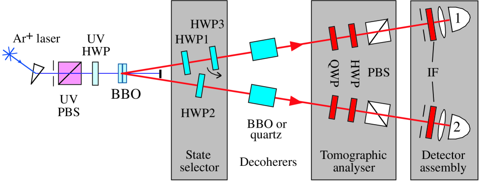
FIG. 1.: Experimental setup for quantum state synthesis.

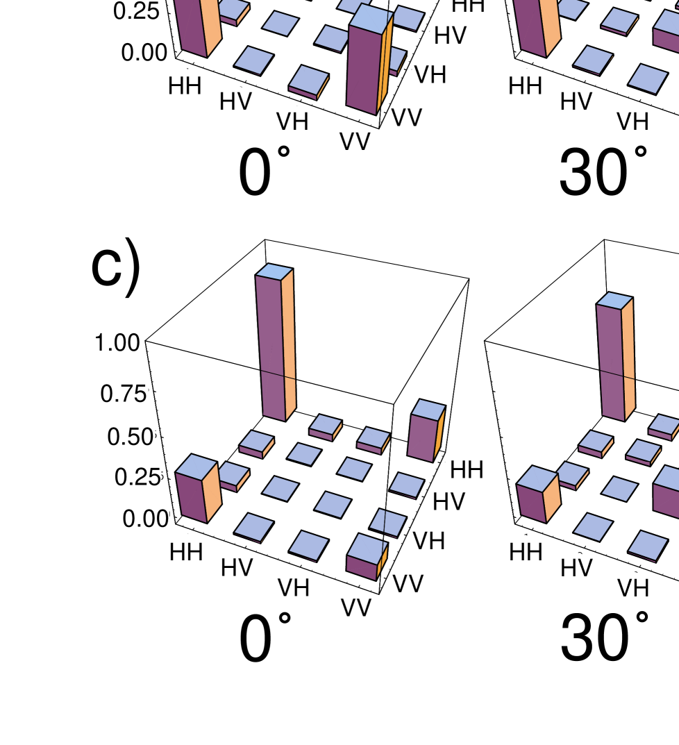
FIG. 2.: States obtained by spatially-based polarisation decoherence. a) i) Input state $(|\rm{HH}\rangle+|\rm{VV}\rangle)/\sqrt{2}$; ii), iii) States after passing through BBO decoherers in one and both arms, respectively. States obtained by temporally-based polarisation decoherence. b) The state, $(|\rm{HH}\rangle+|\rm{VV}\rangle)/\sqrt{2}$, after passing through the state selector ($\theta_{1}=0$, $\theta_{2}$ set as shown) and the quartz decoherers set as described in the text. c) As for b), but with the non-maximally entangled initial state $0.96|\rm{HH}\rangle+0.29|\rm{VV}\rangle$. Only the real components of the density matrices are shown, the imaginary components being at the few percent level or less.

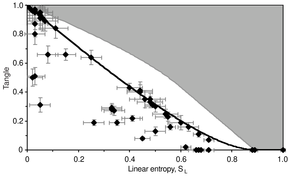
FIG. 3.: Tangle vs linear entropy for 2 qubits. black curve: Werner states. Data points are calculated tangle and linear entropy from a range of measured density matrices. The grey region indicates physically impossible combinations of T and $\rm{S_{L}}$; maximal states (Eq. 1) lie at the boundary of this region.

REFERENCES

- [1] P. W. Shor, in Proc. 35th Ann’l Symp. on Found. Comp. Sci., S. Goldwasser, Ed. (IEEE, Los Alamitos, CA, 1994), p. 116.
- [2] S. Parker, M. B. Plenio, arXiv.quant-phys/0102136 (2001).
- [3] D. P. DiVincenzo, Phys. Rev. A 51, 1015 (1995).
- [4] I. L. Chuang, M. A. Nielsen, Journal of Modern Optics 44, 2455 (1997).
- [5] D. Gottesman, I. L. Chuang, Nature 402, 390 (1999).
- [6] E. Knill, R. Laflamme and G. J. Milburn, Nature 409, 46, (2001).
- [7] Q. A. Turchette, C. J. Hood, W. Lange, H. Mabuchi, H. J. Kimble, Physical Review Letters 75, 4710 (1995).
- [8] K. Mattle, H. Weinfurter, P. G. Kwiat, A. Zeilinger, Physical Review Letters 76, 4656 (1996).
- [9] D. Bouwmeester et al., Nature 390, 575 (1997).
- [10] Q. A. Turchette et al., Physical Review Letters 81, 3631 (1998).
- [11] D. S. Naik, C. G. Peterson, A. G. White, A. J. Berglund, P. G. Kwiat, Physical Review Letters 84, 4733 (2000).
- [12] I. L. Chuang, N. Gershenfeld, M. Kubinec, Physical Review Letters 80, 3408 (1998).
- [13] S. L. Braunstein, et al., Physical Review Letters 83, 1054 (1999).
- [14] H. J. Kimble, quoted in: Physics Today, January (2000).
- [15] A. G. White, D. F. V. James, P. H. Eberhard, P. G., Kwiat, Physical Review Letters 83, 3103 (1999).
- [16] The tangle, T, is directly related to the Entanglement of Formation, E, which is regarded as the canonical measure of entanglement [17, 18]. (Specifically, , where .) For our 2-qubit system we use a normalised form of the linear entropy, , where the state purity is [19]. Note that .
- [17] W. K. Wootters, Physical Review Letters 80, 2245 (1998).
- [18] V. Coffman, J. Kundu, W. K. Wootters, Physical Review A, 61 052306 (2000).
- [19] S. Bose, V. Vedral, V. Physical Review A, 61 040101(R) (2000).
- [20] By looking in coincidence, we restrict ourselves to the two-(and more)-photon section of the Hilbert space, i.e. we can disregard the vacuum component. Two-photon states measured in this manner have been shown to near maximally violate Bell’s inequality [21], indicating that states are near-pure and near-maximally-entangled, i.e. strongly non-classical.
- [21] G. Weihs, T. Jennewein, C. Simon, H. Weinfurter, and A. Zeilinger, Physical Review Letters 81, 5039 (1998).
- [22] P. G. Kwiat, E. Waks, A. G. White, I. Appelbaum, P. H. Eberhard, Physical Review A 60, R773 (1999).
- [23] D. F. V. James, P. G. Kwiat, W. J. Munro, A. G. White, arXiv.quant-ph/0103121 (2001).
- [24] A. J. Berglund, arXiv.quant-phys/0010001 (2000).
- [25] We stress that this principle - tracing over another degree of freedom in a tightly controlled way to induce decoherence - is applicable well beyond our specific experimental system.
- [26] D. A. Lidar, I. L. Chuang, K. B. Whaley., Physical Review Letters 81, 2594 (1998).
- [27] P. G. Kwiat, A. J. Berglund, J. Altepeter, A. G. White, Science 290, 498 (2000).
- [28] P. G. Kwiat, S. Barraza-Lopez, A. Stefanov, N. Gisin, Nature 409, 1014 (2001).
- [29] R. F. Werner, Physical Review A 40, 4277 (1989).
- [30] W. J. Munro, D. F. V. James, P. G. Kwiat, A. G. White, Physical Review Letters, to appear (2001).
- [31] C. H. Bennett, D. P. DiVincenzo, J. A. Smolin, and W. K. Wootters Physical Review A 54, 3824 (1996).
- [32] V. Vedral, M. B. Plenio, M. A. Rippin, and P. L. Knight Physical Review Letters 78, 2275 (1997).
- [33] R. T. Thew, W. J. Munro, Physical Review A 63, 030302(R) (2001).
- [34] R. Cleve, D. Gottesman, H.-K. Lo, Physical Review Letters 82, 648 (1999).
- [35] B. Kane, Nature 393, 133 (1998).
- [36] E. Schrödinger, Proc. Camb. Phil. Soc. 31, 555 (1935).
- [37] W. J. Munro, K. Nemoto, A. G. White, arXiv.quant-phys/quant-ph/0102119 (2001).
- [38] DFVJ wishes to thank the University of Queensland for their hospitality. This work was supported in part by the Australian Research Council (ARC), the US National Security Agency (NSA) and the US Advanced Research and Development Activity (ARDA). Correspondence and request for materials should be addressed to andrew@physics.uq.edu.au.