Contents

toc

Chapter 1

QUANTUM-OPTICAL STATES IN
FINITE-DIMENSIONAL HILBERT SPACE.
I. GENERAL FORMALISM

ADAM MIRANOWICZ

CREST Research Team for Interacting Carrier Electronics, School of Advanced Sciences, The Graduate University for Advanced Studies (SOKEN), Hayama, Kanagawa, Japan and Nonlinear Optics Division, Institute of Physics, Adam Mickiewicz University, Poznań, Poland

WIESŁAW LEOŃSKI

Nonlinear Optics Division, Institute of Physics, Adam Mickiewicz University, Poznań, Poland

NOBUYUKI IMOTO

CREST Research Team for Interacting Carrier Electronics, School of Advanced Sciences, The Graduate University for Advanced Studies (SOKEN), Hayama, Kanagawa, Japan

I.     INTRODUCTION

In the late twentieth century much attention has been paid to the investigation of various quantum-optical states defined in a finite-dimensional Hilbert space of operators, which are bounded and have a discrete spectrum. Yet, the idea of creating finite-dimensional quantum-optical states was conceived much earlier. In fact, back in 1931, Weyl’s formulation of quantum mechanics [1] opened the possibility of studying the dynamics of quantum systems both in infinite-dimensional (ID) and finite-dimensional (FD) Hilbert spaces. Weyl’s approach, generalized by Schwinger [2], is based on the fact that the kinematical structure of a physical system can be expressed by an irreducible Abelian group of unitary representations of system space. For a given finite Abelian group there is a unique class of unitarily equivalent, irreducible representations in FD space. Hence, this formulation has provided the basis for studies of the behavior of the harmonic oscillator in FD Hilbert spaces. In the 1970s, Santhanam and coworkers contributed to the above-mentioned formulation in a series of papers [3]. To describe the interaction of an assembly of two-level atoms with a transverse electromagnetic field, Radcliffe [4] and Arecchi et al. [5] introduced the atomic (or spin) coherent states (also referred to as the directed angular-momentum states [6]) as FD analogs of the conventional optical coherent states (CS) [7, 8, 9]. General formulation of coherent states in FD and ID Hilbert spaces was then developed by Perelomov [10], and Gilmore et al. [11, 12] (see also Refs. [13, 14, 15]). In the 1990s, various quantum-optical states were constructed in FD Hilbert spaces in analogy to those in the ID spaces. In particular, (1) various kinds of FD coherent states [16]–[24], (2) FD displaced number states [21], (3) FD even and odd coherent states [25, 21, 24], (4) FD phase states [26], (5) FD phase coherent states (also referred to as coherent phase states) [27]–[30], (6) FD squeezed states [31]–[34], (7) FD displaced phase states [28], or (8) FD even and odd phase coherent states [35].

The interest in the FD quantum-optical states has been stimulated by the progress in quantum-optical state preparation and measurement techniques [36], in particular, by the development of the discrete quantum-state tomography [37]–[42]. There are several other reasons for studying states in FD spaces.

1. We can treat FD quantum-optical states as those of a real single-mode electromagnetic field, which fulfill the condition of truncated Fock expansion. These states can directly be generated by the truncation schemes (the quantum scissors) proposed by Pegg et al. [44] and then generalized by other authors [45, 46, 47]. Alternatively, one can analyze states obtained by a direct truncation of operators rather then of their Fock expansion. Such an operator truncation scheme, proposed by Leoński et al. [48, 49, 50], will be discussed in detail in the next chapter [51].

2. The formalism of FD quantum-optical states is applicable to other systems described by the FD models as well, such as spin systems or ensembles of two-level atoms or quantum dots. In such cases we should talk about, for instance, the $z$-component of the spin and its azimuthal orientation rather than about the photon number and phase. However, the states studied here were first discussed in the quantum-optical papers and we also will keep the terminology of quantum optics.

3. This analysis gives us a deeper insight into the Pegg–Barnett phase formalism [26] (for a review, see Ref. [43]) of the Hermitian optical phase operator constructed in ($s+1$)-dimensional state Hilbert space. The key idea of the Pegg–Barnett procedure is to calculate all the physical quantities such as expectation values or variances in the FD space and only then to take the limit of $s\rightarrow\infty$. Bužek et al. [16] pointed out that all quantities (in particular states) analyzed within the Pegg–Barnett formalism, should properly be defined in the same ($s+1$)-dimensional state space before finally going over into the infinite limit. So, for better understanding of the Pegg–Barnett formalism, it is useful to construct finite-dimensional states and to know what exactly happens before taking the limit.

In this chapter, we apply a discrete Wigner function to describe FD quantum-optical states. Wigner function is widely used in nonrelativistic quantum mechanics as an alternative to the density matrix of quantum systems [52]. Although the original Wigner function applies only to systems with continuous degrees of freedom, it can be generalized for finite-state systems as well [53]. Discrete Wigner function for spin-$\frac{1}{2}$ systems was introduced by O’Connell and Wigner [54] and generalized for arbitrary spins by Wootters [55]. His definition takes the simplest form for prime-number-dimensional systems. A similar construction of a discrete Wigner function for odd-dimensional systems was suggested by a Cohendet et al. [56]. A number-phase discrete Wigner function, a special case of the Wootters definition, was analyzed in detail by Vaccaro and Pegg [57]. Another definition of Wigner function (for odd dimensions equivalent to that of Wootters) was proposed by Leonhardt [37]. This approach can readily be generalized to define a discrete Husimi $Q$ function or, moreover, discrete parameterized phase-space functions as was studied by Opatrný et al. [58, 59]. Another generalization of discrete Wigner function for Schwinger’s FD periodic Hilbert space was analyzed by, for instance, Hakioǧlu [60]. The Wigner function approach to FD systems can be developed from basic principles as was shown, for example, by Wootters [55], Leonhardt [37], Lukš and Peřinová [61], or Luis and Peřina [62]. Discrete Wigner function has successfully been applied to quantum-state tomography of FD systems [37] (for a review, see Ref. [42]).

This work is intended as an attempt to present two essentially different constructions of harmonic oscillator states in a FD Hilbert space. We propose some new definitions of the states and find their explicit forms in the Fock representation. For the convenience of the reader, we also bring together several known FD quantum-optical states, thus making our exposition more self-contained. We shall discuss FD coherent states, FD phase coherent states, FD displaced number states, FD Schrödinger cats, and FD squeezed vacuum. We shall show some intriguing properties of the states with the help of the discrete Wigner function.

II.    FD HILBERT SPACE

We shall discuss various states constructed in FD Hilbert space of harmonic oscillator. Let us denote by ${\mathcal{}H}^{(s)}$ the ($s+1$)-dimensional Hilbert space spanned by number states $\{|0\rangle,|1\rangle,\dots,|s\rangle\}$ fulfilling the completeness and orthogonality relations

$$\hat{1}_{s}=\sum_{n=0}^{s}|n\rangle\langle n|\,,\qquad\langle n|m\rangle=\delta_{n,m}$$ (1.1)

where $n,m=0,\dots,s$ and $\hat{1}_{s}$ is the unit operator in ${\mathcal{}H}^{(s)}$. Thus, arbitrary quantum-optical pure state in the FD Hilbert space can be defined by its Fock expansion

$$|\psi{\rangle\!_{(s)}}=\;\sum_{n=0}^{s}C_{n}^{(s)}|n\rangle\equiv\;\sum_{n=0}^{s}b_{n}^{(s)}{\mathrm{e}}^{{\mathrm{i}}\varphi_{n}}|n\rangle$$ (1.2)

where $C_{n}^{(s)}=b_{n}^{(s)}{\mathrm{e}}^{{\mathrm{i}}\varphi_{n}}$ and $b_{n}^{(s)}$ are real superposition coefficients fulfilling the normalization condition

$${{}_{(s)}\!\langle}\psi|\psi{\rangle\!_{(s)}}=\sum_{n=0}^{s}[b_{n}^{(s)}]^{2}=1$$ (1.3)

for arbitrary dimension $(s+1)$ of Hilbert space. It is sometimes useful to represent the optical state, given by (1.2), via the phase states defined to be [26]

$$|\theta_{m}\rangle\equiv|\theta_{m}{\rangle\!_{(s)}}=\frac{1}{\sqrt{s+1}}\sum_{n=0}^{s}\exp({\mathrm{i}}n\theta_{m})|n\rangle$$ (1.4)

with the phases $\theta_{m}$ given by

$$\theta_{m}=\theta_{0}+\frac{2\pi}{s+1}\,m$$ (1.5)

where $\theta_{0}$ is the initial reference phase and $m=0,\dots,s$. States (1.4) also form a complete and orthonormal basis:

$$\hat{1}_{s}=\sum_{m=0}^{s}|\theta_{m}\rangle\langle\theta_{m}|\,,\qquad\langle\theta_{m}|\theta_{n}\rangle=\delta_{m,n}$$ (1.6)

The phase states were applied by Pegg and Barnett in their definition of the Hermitian quantum-optical phase operator [26]

$${\hat{\Phi}}_{s} \equiv {\hat{\Phi}}_{s}(\theta_{0})\;=\;\sum_{m=1}^{s}\theta_{m}|\theta_{m}\rangle\langle\theta_{m}|$$ (1.7)

The phase states can also be used in construction of a discrete Wigner function as will be described in Section III. The FD annihilation and creation operators in ${\mathcal{}H}^{(s)}$ are defined by

$$\hat{a}_{s} = \sum_{n=1}^{s}\sqrt{n}|n-1\rangle\langle n|$$

$$\hat{a}_{s}^{\dagger} = \sum_{n=1}^{s}\sqrt{n}|n\rangle\langle n-1|$$ (1.8)

The FD and ID annihilation operators act on a number state in the same manner. However, the actions of the creation operators on $|n\rangle$ are different in ${\mathcal{}H}^{(s)}$ and ${\mathcal{}H}^{(\infty)}$. Equation (1.8) implies that

$$({\hat{a}}_{s}^{\dagger})^{k}|n\rangle=0$$ (1.9)

if $n+k>s$. By contrast, the action of the ID creation operator (in any power) on $|n\rangle$ gives always nonzero result. The commutation relation for the annihilation and creation operators in ${\mathcal{}H}^{(s)}$ reads as

$$[{\hat{a}_{s}},{\hat{a}_{s}^{\dagger}]=1-(s+1)|s\rangle\langle s|}$$ (1.10)

which differs from the conventional boson canonical relation in ${\mathcal{}H}^{(\infty)}$. Thus, $\hat{a}_{s}$ and $\hat{a}_{s}^{\dagger}$ are not related to the Weyl–Heisenberg algebra. Even the double commutators $[\hat{a}_{s},[\hat{a}_{s},\hat{a}_{s}^{\dagger}]]$ and $[\hat{a}_{s}^{\dagger},[\hat{a}_{s},\hat{a}_{s}^{\dagger}]]$ do not vanish precluding the application of the Baker-Hausdorff theorem. These properties of the FD annihilation and creation operators considerably complicate analytical approaches to the quantum mechanics in ${\mathcal{}H}^{(s)}$, including the explicit construction of the FD harmonic oscillator states.

Creation and annihilation of phase quanta in FD Hilbert space can be defined in a close analogy to the creation and annihilation of photons, as given by Eq. (1.8). Phase annihilation, $\hat{\phi}_{s}$, and phase creation, $\hat{\phi}_{s}^{\dagger}$, operators can be introduced with the help of the relation $\hat{\Phi}_{s}=\hat{\phi}_{s}^{\dagger}\hat{\phi}_{s}$ for the Pegg–Barnett phase operator, given by (1.7). The FD phase annihilation and creation operators in the phase-state basis, have the following form [16]

$$\hat{\phi}_{s}\;\equiv\;\hat{\phi}_{s}(\theta_{0}) = \sum_{m=1}^{s}\sqrt{\theta_{m}}|\theta_{m-1}\rangle\langle\theta_{m}|+\sqrt{\theta_{0}}|\theta_{s}\rangle\langle\theta_{0}|$$

$$\hat{\phi}_{s}^{\dagger}\;\equiv\;\hat{\phi}_{s}^{\dagger}(\theta_{0}) = \sum_{m=1}^{s}\sqrt{\theta_{m}}|\theta_{m}\rangle\langle\theta_{m-1}|+\sqrt{\theta_{0}}|\theta_{0}\rangle\langle\theta_{s}|$$ (1.11)

respectively. Their commutator is

$$[\hat{\phi}_{s},\hat{\phi}_{s}^{\dagger}] = \frac{2\pi}{s+1}-2\pi|\theta_{s}\rangle\langle\theta_{s}|$$ (1.12)

The phase annihilation and creation operators act on the phase states in a similar way (particularly for $\theta_{0}=0$) as the conventional (photon-number) annihilation and creation operators act on number states.

III.  DISCRETE WIGNER FUNCTION FOR FD STATES

The expression of quantum-optical states by quasidistributions enables a very intuitive description of their properties. Here, we give a general definition of the discrete Wigner-function. We also present its graphical representations for several FD quantum-optical states, often discussed in recent works. The Wigner function will be studied in greater detail in the following sections.

The number–phase characteristic function in ${\mathcal{}H}^{(s)}$ can be defined as [37]

$$C_{s}(\nu,\theta_{\mu})=\sum_{m=0}^{s}\exp\left(-\frac{4\pi{\mathrm{i}}}{s+1}\nu(m+\mu)\right)\langle\theta_{m}|\hat{\rho}|\theta_{m+2\mu}\rangle$$ (1.13)

in terms of the phase states (1.4). A discrete Fourier transform applied to $C_{s}(\nu,\theta_{\mu})$ leads to the following discrete Wigner function (for brevity referred to as the $W$ function) for phase and number

$$W_{s}(n,\theta_{m})=\frac{1}{\left(s+1\right)^{2}}\sum_{\nu=0}^{s}\sum_{\mu=0}^{s}\exp\left(\frac{4\pi{\mathrm{i}}}{s+1}(n\mu+\nu m)\right)C_{s}(\nu,\theta_{\mu})$$ (1.14)

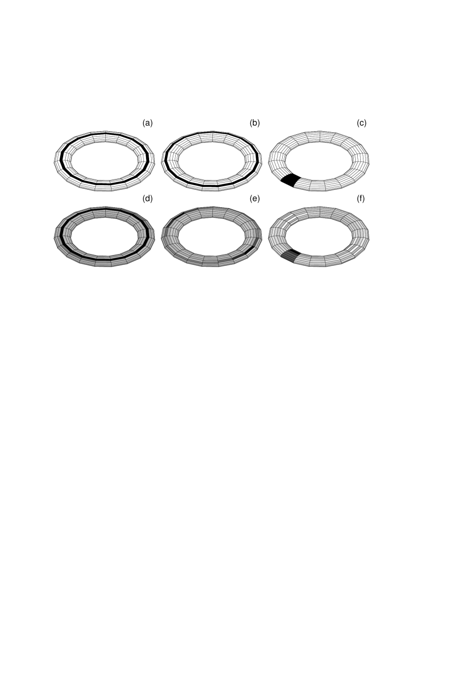
Fig. 1.1: Examples of discrete Wigner function on a torus in 19-dimensional Hilbert space ($s=18$): (a) vacuum $|0\rangle$; (b) single-photon number state $|1\rangle$; (c) FD preferred phase state (“phase vacuum”) $|\theta_{0}\rangle_{(s)}$; (d) FD coherent state, $|\alpha\rangle_{(s)}\approx|\overline{\alpha}\rangle_{(s)}$; (e) FD displaced number state, $|\alpha,1\rangle_{(s)}\approx|\overline{\alpha},1\rangle_{(s)}$; (f) FD phase coherent state, $|\beta,\theta_{0}\rangle_{(s)}\approx|\overline{\beta},\theta_{0}\rangle_{(s)}$, with equal displacement parameters, $\alpha=\overline{\alpha}=\beta=\overline{\beta}=0.5$ and $\theta_{0}=0$. The darker is a region, the higher is the value of the Wigner function.

or, explicitly, as [55, 37]

$$W_{s}(n,\theta_{m})=\frac{1}{s+1}\sum_{\mu=0}^{s}\exp\left(\frac{4\pi{\mathrm{i}}}{s+1}n\mu\right)\langle\theta_{m-\mu}|\hat{\rho}|\theta_{m+\mu}\rangle$$ (1.15)

The Wigner function $W_{s}(n,\theta_{m})$ is periodic both in $n$ and $\theta_{m}$:

$$W_{s}(n,\theta_{m}) = W_{s}(n\pm\{s+1\},\theta_{m})$$ (1.16)

$$= W_{s}(n,\theta_{m\pm(s+1)})$$

$$= W_{s}(n,\theta_{m}\pm 2\pi)$$

Thus, it is represented graphically on torus [20]. The Wigner function for any FD pure state of the form (1.2) can be expressed as follows [57]

$$W_{s}(n,\theta_{m})=\frac{1}{s+1}\left\{\sum_{k=0}^{M}b^{(s)}_{k}b^{(s)}_{M-k}\exp[{\mathrm{i}}(2k-M)\theta_{m}+\varphi_{M-k}-\varphi_{k}]\right.\quad$$

$$\;+\!\!\!\!\left.\sum_{k=M+1}^{s}b^{(s)}_{k}b^{(s)}_{M-k+s+1}\exp[{\mathrm{i}}(2k-M-s-1)\theta_{m}+\varphi_{M-k+s+1}-\varphi_{k}]\right\}$$ (1.17)

in terms of the decomposition coefficients $b^{(s)}_{k}$ and $M\equiv 2n\ \mbox{mod}(s+1)$. Several graphs of these functions of various states are presented here (Fig. 1.1) and in the next sections. The physical interpretation of the Wigner functions is based on the fact that the marginal sum of their values over a generalized line gives the probability that the system will be in some state [55, 37]. In the ID Hilbert space, where the $W$ function arguments are continuous (quadratures $X$ and $Y$), a marginal integral along any straight line $aX+bY+c=0$ is nonnegative and can be considered to be the probability. A similar situation arises in the FD case; we can define lines as sets of discrete points $(n,\theta_{m})$, or equivalently $(n,m)$, for which the relation $(an+bm+c)\mbox{mod}N=0$ holds (here, $a,b,c$ are integers). Again, sums of the discrete $W$ function values on such sets are nonnegative. The mod $(s+1)$ relations are essential and are connected to some periodic properties of the discrete $W$ function — the maximum value of each argument ($m$ or $n$) is topologically followed by its minimum (zero in our case). This means that the discrete $W$ function is defined on a torus (or more precisely on a discrete set of points of a torus). The “lines” are then points of closed toroidal spirals or, in a special case, points of a circle. The periodic property is quite natural for the phase index $m$, but may seem strange for the photon number $n$. In the next sections, we shall draw attention to some consequences of the periodicity in $n$ for generalized coherent states, for instance.

One aim of this chapter is to show graphs of the discrete $W$ functions for FD quantum-optical states. Because of the discreteness of the arguments, the $W$ function graph should be a histogram. However, two-dimensional projections of such three-dimensional histograms could be very confusing. Therefore, for better legibility of the graphs, we have decided to depict them topographically. The darker is a region, the higher is the value of the $W$ function it represents. Moreover, negative values of the $W$ function are marked by crosses. As mentioned above, the most natural way of presenting the discrete $W$ function graphs is to construct them on toruses. A few simple examples of the toroidal discrete Wigner functions are given in Fig. 1.1. Unfortunately, this graphical representation is seldom transparent enough for its interpretation. In what follows we shall work with two-dimensional graphs. Here, one should keep in mind that some consequences of the periodicity in $n$ and $m$ can appear: for instance, some peaks can be located partially at the outer boundary at $n\approx s$ (or $m\approx s$) and can “continue” near the center $n\approx 0$ (or $m\approx 0$). In the next section, the $W$ functions of various FD states will be presented.

For a better understanding of the discrete Wigner function, let us recall its close correspondence to the discrete Pegg–Barnett phase distribution [26]

$$P_{s}(\theta_{m})=\sum_{n=0}^{s}W_{s}(n,\theta_{m})=\left|{{}_{(s)}\!\langle}\theta_{m}|\psi{\rangle\!_{(s)}}\right|^{2}$$ (1.18)

and to the photon-number distribution

$$P_{s}(n) = \sum_{m=0}^{s}W_{s}(n,\theta_{m})=\left|\langle n|\psi{\rangle\!_{(s)}}\right|^{2}=|b^{(s)}_{n}|^{2}$$ (1.19)

Thus, the sum of the $W$ function values, at constant $\theta_{m}$, over all $n$ values gives the probability of the phase $\theta_{m}$ and, analogously, the sum with constant $n$ over all arguments $\theta_{m}$ gives the probability of $n$ photons — at least in systems, which are fully described by finite-number state models. If we want to interpret our results as describing states of a usual one-mode field under the condition that all Fock components of $|n\rangle$ with $n>s$ are absent, then the real phase probability distribution is obviously continuous. Let us briefly discuss its connection to the obtained discrete distribution. If $s$ is greater than or equal to the largest Fock state component of a given state, which by definition is our case, then the discrete probabilities (from the discrete Wigner phase marginal) are proportional to the values of the continuous phase probability distribution in the discrete set of points (1.5). One can easily obtain other values also, although not directly. We could use a FD version of the sampling theorem — if the $n$ distribution is limited, then for description a state in the phase representation only a discrete set of phase amplitudes is necessary. It is clear that the $(s+1)^{2}$ real values of the discrete $W$ function yield the same information as the $(s+1)^{2}$ real nonzero parameters of the related density matrix.

IV.   FD COHERENT STATES

The most common states in quantum optics are the coherent states (CS) introduced by Schrödinger [7] in connection with classical states of the quantum harmonic oscillator. First modern description and specific application of CS is due to Glauber [8] and Sudarshan [9]. The literature on CS and their generalizations is truly prodigious and has been summarized in a number of excellent monographs [10, 13, 14, 63] and reviews [12]. There are several ways of generalizing the conventional ID coherent states to comprise the FD case. It is possible to define CS using the concept of Lie group representations [63], or to postulate the validity of some properties of the ID CS for their FD analogs. In this chapter, we are interested in two definitions of the latter kind. First, CS in a FD space are usually treated as the displaced vacuum, where the displacement operator is defined analogously to the conventional displacement operator in the ID space (the Glauber treatment of CS [8]). This idea was applied in the work of Bužek and co-workers [16] and further studied by Miranowicz et al. [18] and Opatrný et al. [20]. Here, we refer to such states as the generalized CS. Another definition is based on the postulate that the Fock expansion of the FD CS is be equal to the truncated expansion of the conventional ID CS. This approach was extensively developed by Kuang et al. [17] and Opatrný et al. [20]. Here, we shall refer to CS of this kind as the truncated CS. An experimental scheme, known as the quantum scissors, for generation of the truncated CS was proposed by Pegg et al. [44]. Quantum scissors were generalized by Koniorczyk et al. [45], Paris [46], and Miranowicz et al. [47]. A physical system for preparation of the generalized CS was proposed by Leoński [49] (see also Ref. [50]) as a modification of the Fock state engineering technique of Leoński and Tanaś [48]. These schemes are presented in the next chapter [51].

A.   Generalized Coherent States

Glauber [8] constructed coherent states in the ID Hilbert space by applying the displacement operator $\hat{D}(\alpha,\alpha^{*})\equiv\exp(\alpha\hat{a}^{\dagger}-\alpha^{*}\hat{a})$ on vacuum state $|0\rangle$. Analogously, one can define the generalized coherent state [16]

$$|\alpha{\rangle\!_{(s)}} = \hat{D}_{s}(\alpha,\alpha^{*})|0\rangle$$ (1.20)

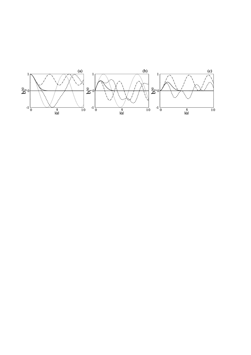
Fig. 1.2: Generalized coherent states: The superposition coefficients $b^{(s)}_{n}$ for $|\alpha\rangle_{(s)}$ versus displacement parameter amplitude $|\alpha|$ for: (a) $n$=0, (b) $n$=1, and (c) $n$=2 in the Hilbert spaces of different dimensionality: $s=1$ (dotted), $s=2$ (dot–dashed), $s=3$ (dashed), and $s=\infty$ (solid curves).

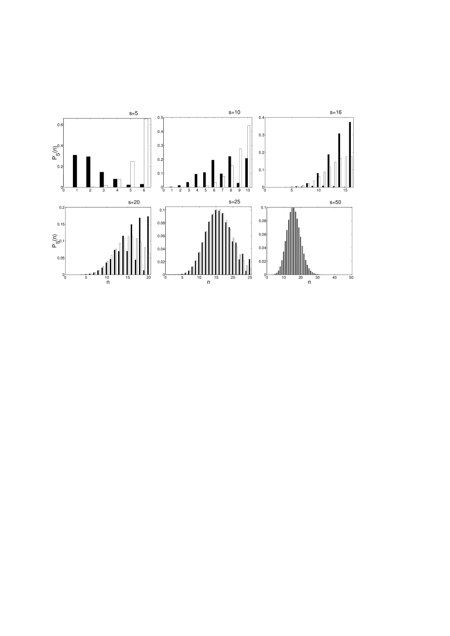
Fig. 1.3: Generalized coherent states (black bars) versus truncated coherent states (white bars): photon-number distribution $P_{s}(n)$ as a function of $n$ in FD Hilbert spaces with $s=5,\cdots,50$ for the same displacement parameters $\alpha=\overline{\alpha}=4$.

constructed in the FD Hilbert space by the action of the generalized FD given by displacement operator

$$\hat{D}_{s}(\alpha,\alpha^{*}) = \exp\big{[}\alpha\hat{a}_{s}^{\dagger}-\alpha^{*}\hat{a}_{s}\big{]}$$ (1.21)

where the FD annihilation and creation operators are given by (1.8). Definitions of CS based on displacement operators are usually applied in various generalizations of CS [4, 5, 10, 12, 16, 18]. The generalized coherent state, $|\alpha{\rangle\!_{(s)}}$ with $\alpha=|\alpha|\exp({\mathrm{i}}\varphi)$, has the following Fock expansion [18]

$$|\alpha{\rangle\!_{(s)}}=\sum_{n=0}^{s}{\mathrm{e}}^{{\mathrm{i}}n\varphi}\,b^{(s)}_{n}\,|n\rangle$$ (1.22)

where

$$b^{(s)}_{n} = \frac{s!}{s+1}\frac{(-{\mathrm{i}})^{n}}{\sqrt{n!}}\,\sum_{k=0}^{s}{\mathrm{e}}^{{\mathrm{i}}x_{k}|\alpha|}\,\frac{{\mathrm{H}e}_{n}(x_{k})}{{\mathrm{H}e}_{s}^{2}(x_{k})}$$ (1.23)

Here, $x_{k}\equiv x_{k}^{(s+1)}$ are the roots, $\mbox{He}_{s+1}(x_{k})=0$, of the Hermite polynomial $\mbox{He}_{n}(x)\equiv 2^{-n/2}\mbox{H}_{n}(x/\sqrt{2})$. A method for deriving the coefficients (1.23) is presented in the Appendix. In the special cases for $s=1,2,3$, the generalized CS are as follows

$$|\alpha{\rangle\!_{(1)}} = \cos|\alpha||0\rangle+{\mathrm{e}}^{{\mathrm{i}}\varphi}\sin|\alpha||1\rangle$$ (1.24)

$$|\alpha{\rangle\!_{(2)}} = \frac{1}{3}\Big{[}\cos\big{(}\sqrt{3}|\alpha|\big{)}+2\Big{]}|0\rangle+\frac{1}{\sqrt{3}}\,{\mathrm{e}}^{{\mathrm{i}}\varphi}\sin\big{(}\sqrt{3}|\alpha|\big{)}|1\rangle$$ (1.25)

$$+\frac{\sqrt{2}}{3}\,{\mathrm{e}}^{2{\mathrm{i}}\varphi}\left[1-\cos\big{(}\sqrt{3}|\alpha|\big{)}\right]|2\rangle$$

$$|\alpha{\rangle\!_{(3)}} = \frac{x^{2}_{2}{\mathsf{c}}_{1}+x^{2}_{1}{\mathsf{c}}_{2}}{2x^{2}_{1}x^{2}_{2}}|0\rangle+\frac{x_{2}{\mathsf{s}}_{1}+x_{1}{\mathsf{s}}_{2}}{2x_{1}x_{2}}\,{\mathrm{e}}^{{\mathrm{i}}\varphi}|1\rangle$$ (1.26)

$$-\frac{{\mathsf{c}}_{1}-{\mathsf{c}}_{2}}{2\sqrt{3}}\,{\mathrm{e}}^{2{\mathrm{i}}\varphi}|2\rangle-\frac{x_{2}{\mathsf{s}}_{1}-x_{1}{\mathsf{s}}_{2}}{2x_{1}x_{2}}\,{\mathrm{e}}^{3{\mathrm{i}}\varphi}|3\rangle$$

where ${\mathsf{s}}_{k}=\sin(x^{(4)}_{k}|\alpha|)$ and ${\mathsf{c}}_{k}=\cos(x^{(4)}_{k}|\alpha|)$ are functions of the roots $x_{1,2}^{(4)}=\sqrt{3\pm\sqrt{6}}$. The state (1.24) in the two-dimensional Hilbert space will be studied in greater detail in Section IV.C. The simplicity of (1.24) comes from the fact that the only nonvanishing coefficients $d_{nk}^{(1)}$, given by Eq. (A.7), are equal to unity. In Fig. 1.2, the coefficients $b_{n}^{(s)}$ are presented in their dependence on the parameter $|\alpha|$ for $s=1,2,3$ and $s=\infty$. It is seen that the coefficients (1.23) are periodic (for $s$=1, 2) or quasiperiodic (for higher $s$) in $|{\overline{\alpha}\,}|$. The generalized CS go over into the conventional CS in the limit of $s\rightarrow\infty$. This conclusion can be drawn by analyzing Fig. 1.3, where the photon-number distribution $P_{s}(n)=|b_{n}^{(s)}|^{2}$ for the generalized CS is presented for different values of $s$ and fixed $\alpha=4$. The differences between $|\alpha{\rangle\!_{(s)}}$ and $|\alpha{\rangle\!_{(\infty)}}$ vanish even for $s=50$ on the scale of Fig. 1.3. In order to prove this property analytically, let us expand the scalar product between $|\alpha{\rangle\!_{(s)}}$ and $|\alpha{\rangle\!_{(\infty)}}$ in series of parameter $|\alpha|$. One finds the following power series expansions [20]

$${{}_{(\infty)}\!\langle}\alpha|\alpha{\rangle\!_{(1)}} = 1-{\textstyle\frac{1}{4}\,}|\alpha|^{4}+{\textstyle\frac{1}{9}\,}|\alpha|^{6}-{\mathcal{}O}(|\alpha|^{8})$$

$${{}_{(\infty)}\!\langle}\alpha|\alpha{\rangle\!_{(2)}} = 1-{\textstyle\frac{1}{12}\,}|\alpha|^{6}+{\textstyle\frac{3}{64}\,}|\alpha|^{8}-{\mathcal{}O}(|\alpha|^{10})$$

$${{}_{(\infty)}\!\langle}\alpha|\alpha{\rangle\!_{(3)}} = 1-{\textstyle\frac{1}{48}\,}|\alpha|^{8}+{\textstyle\frac{1}{75}\,}|\alpha|^{10}-{\mathcal{}O}(|\alpha|^{12})$$ (1.27)

for particular values of $s$. We see that, with increasing dimension, the generalized CS approach the conventional CS as

$${{}_{(\infty)}\!\langle}\alpha|\alpha{\rangle\!_{(s)}} = 1-\frac{|\alpha|^{2(s+1)}}{2\,(s+1)!}+{\mathcal{}O}(|\alpha|^{2(s+2)})$$ (1.28)

for $|\alpha|^{2}\ll s$.

On insertion of the coefficients (1.23) into the general formula (1.17), we get the Wigner function for $|\alpha{\rangle\!_{(s)}}$ in the form

$$W_{s}(n,\theta_{m}) = \sum_{k=M+1}^{s}\frac{\exp[{\mathrm{i}}(2k-M-s-1)(\theta_{m}-\varphi+\pi/2)]}{[k!(M-k+s+1)!]^{1/2}}G_{1k}$$ (1.29)

$$+\!\sum_{k=0}^{M}\frac{\exp[{\mathrm{i}}(2k-M)(\theta_{m}-\varphi+\pi/2)]}{[k!(M-k)!]^{1/2}}G_{0k}$$

where

$$G_{\eta k}=\frac{(s!)^{2}}{(s+1)^{3}}\sum_{p=0}^{s}\sum_{q=0}^{s}\exp[{\mathrm{i}}(x_{q}-x_{p})|\alpha|]\frac{\mbox{He}_{k}(x_{p})\mbox{He}_{M-k+\eta(s+1)}(x_{q})}{[\mbox{He}_{s}(x_{p})\mbox{He}_{s}(x_{q})]^{2}}$$ (1.30)

with $\eta=0,1$. By writing Eq. (1.29) in a form more similar to the Vaccaro–Pegg expression, we arrive at

$$W_{s}(n,\theta_{m}) = \sum_{k=2n+1}^{s}(-1)^{k-n-s/2}\;\frac{\sin[(2k-2n-s-1)(\theta_{m}-\varphi)]}{[k!(2n-k+s+1)!]^{1/2}}G_{1k}$$ (1.31)

$$+\sum_{k=0}^{2n}(-1)^{k-n}\;\frac{\cos[(2k-2n)(\theta_{m}-\varphi)]}{[k!(2n-k)!]^{1/2}}G_{0k}$$

for $n\leq s/2$, and

$$W_{s}(n,\theta_{m}) = \sum_{k=0}^{2n-s-1}(-1)^{k-n-s/2}\;\frac{\sin[(2k-2n+s+1)(\theta_{m}-\varphi)]}{[k!(2n-k-s-1)!]^{1/2}}G_{0k}$$ (1.32)

$$+\;\sum_{k=2n-s}^{s}(-1)^{k-n}\;\frac{\cos[(2k-2n)(\theta_{m}-\varphi)]}{[k!(2n-k)!]^{1/2}}G_{1k}$$

for $n>s/2$. As readily seen, we cannot generally factorize this function into a product of amplitude $|\alpha|$- and phase $\varphi$- dependent parts. The Wigner functions for the generalized CS are presented for $s=18$ in Fig. 1.4. We observe the following behavior of the Wigner function. The shape of the respective graph is approximately periodic (referred to as the quasiperiodic) in the parameter $|\alpha|$ with quasiperiod $T_{s}\approx 8.8$. We find that for small $|{\overline{\alpha}\,}|$ the shape is essentially the same as that described in Ref. [57] — for $n\leq s/2$, there are two peaks for opposite phases, whereas for $n>s/2$ we observe a peak and an antipeak. Note, the peaks at the borders are artificially split up in our Cartesian representation of the Wigner function. The peaks or antipeaks are located at such positions that on summing the $W$ function with constant $n$ (or $\theta_{m}$) over $\theta_{m}$ (or $n$), we get the probability distribution of $n$ (or $\theta_{m}$, respectively). Then, with increasing $|\alpha|$, interesting oscillations in photon number appear. Their culmination is at $|\alpha|=T_{s}/2$ (Fig. 1.4c), where only even photon numbers are present. For this value of $\alpha$, the generalized coherent state approaches an even CS, namely, the case of a Schrödinger cat state, which will be described in detail in Section IV.D.1. By further enlarging $|\alpha|$, the $W$ function returns to its previous shapes through the transition regime (for $|\alpha|\approx 2T_{s}/3$ in Fig. 1.4d) to the case of the inner two-peak and outer peak–antipeak structure, similar to the Vaccaro–Pegg results. For $|\alpha|\approx 5T_{s}/6$ as given in Fig. 1.4e, the $W$ function is very similar to that presented in Fig. 1.4a for $|\alpha|\approx T_{s}/6$, but with opposite phase. Finally, for $|\alpha|=T_{s}$ as presented in Fig. 1.4f, we arrive at an almost vacuum state. By further increasing $|\alpha|$, these shapes of the $W$ function graph reappeared for several quasiperiods $T_{s}$. Similar behavior can be observed also for other values of $s$.

This quasiperiodicity can be explained as follows. By applying the fitting procedure, based on the WKB (Wentzel–Kramers–Brillouin) method, one can find that the smallest positive root $x_{1}\equiv x_{1}^{(s+1)}$ of the Hermite polynomial He${}_{s+1}(x)$ is approximately equal to

$$x_{1}^{(s+1)}\approx\frac{2\pi}{\sqrt{4s+6}}$$ (1.33)

(for even $s$). Besides, it is well known that the nearest-to-zero roots of the Hermite polynomials are approximately equidistant. Thus, their difference $\Delta x\equiv x_{k+1}-x_{k}$ is approximately given by (1.33), which is 0.71 for $s=18$. The predominant terms of the sum in (1.23) depend on $|\alpha|$ approximately as $\exp({\mathrm{i}}g\Delta x|\alpha|)$, where $g=0,\pm 1,\pm 2,\dots$. These exponential functions are quasiperiodic with approximate mean period (referred to as the quasiperiod) given by [20, 64]

$$T_{s}\approx\sqrt{4s+6}$$ (1.34)

for even $s$. From Eq. (1.34), the quasiperiod for $s$=18 is approximately equal to $8.8$. For odd $n$, the property $\mbox{He}_{n}(-x_{k})=(-1)^{n}\mbox{He}_{n}(x_{k})$ holds. On the other hand, the odd coefficients $n$ in the sum (1.23) contain sine functions, which are zero in the middle of their period. Therefore, for $|\alpha|=T_{s}/2$, the odd $n$ terms almost disappear and we get approximately an even coherent state. We analyze in detail the $W$ functions for even $s$ only. Nonetheless, for completeness of our discussion, we give the explicit approximate expression for the quasiperiod

$$T_{s}\approx 2\sqrt{4s+6}$$ (1.35)

for odd $s$, which is twice larger than the quasiperiod given by (1.34) for a chosen value of $s$.

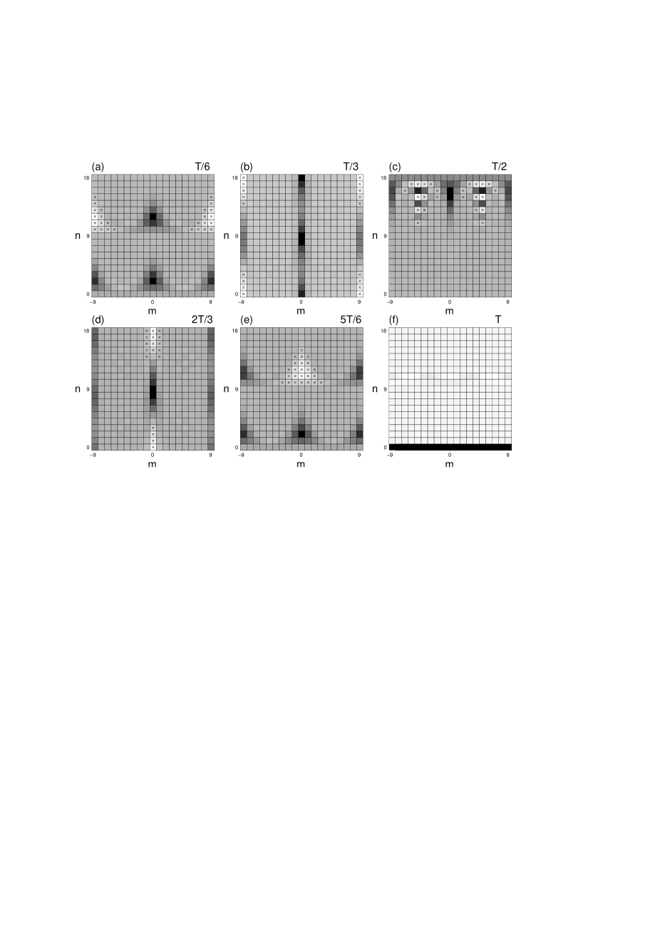
Fig. 1.4: Generalized coherent states: Wigner function $W_{s}(n,\theta_{m})$ in FD Hilbert space with $s=18$ for $|\alpha\rangle_{(18)}$ with different values of displacement parameter $\alpha$, chosen as fractions of the quasiperiod $T\equiv T_{18}\approx 8.8$. As in Fig. 1.1, higher values of Wigner function are depicted darker. Negative regions are marked additionally by crosses.

B.   Truncated Coherent States

Kuang et al. [17] defined the normalized FD coherent states by truncating the Fock expansion of the conventional ID coherent states or equivalently by the action of the operator $\exp({\overline{\alpha}\,}{\hat{a}}^{\dagger})$ (with proper normalization) on vacuum state. The Kuang et al. approach is similar to the Vaccaro–Pegg treatment [57] of the Wigner function for CS. The state $|{\overline{\alpha}\,}{\rangle\!_{(s)}}$, where ${\overline{\alpha}\,}=|{\overline{\alpha}\,}|\exp({\mathrm{i}}\varphi)$, can be defined by its Fock expansion [17]

$$|{\overline{\alpha}\,}{\rangle\!_{(s)}}={\mathcal{}N}_{s}\exp({\overline{\alpha}\,}{\hat{a}}_{s}^{\dagger})\,|0\rangle=\sum_{n=0}^{s}b^{(s)}_{n}\,|n\rangle$$ (1.36)

with the Poissonian superposition coefficients

$$b^{(s)}_{n}={\mathcal{}N}_{s}\sum_{n=0}^{s}\frac{\overline{\alpha}^{n}}{\sqrt{n!}}$$ (1.37)

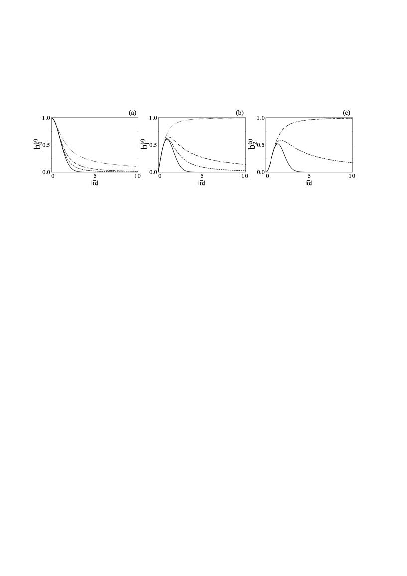
Fig. 1.5: Truncated coherent states: Superposition coefficients ${b}^{(s)}_{n}$ of $|\overline{\alpha}\rangle_{(s)}$ versus displacement parameter amplitude $|\overline{\alpha}|$ for the same cases as in Fig. 1.2.

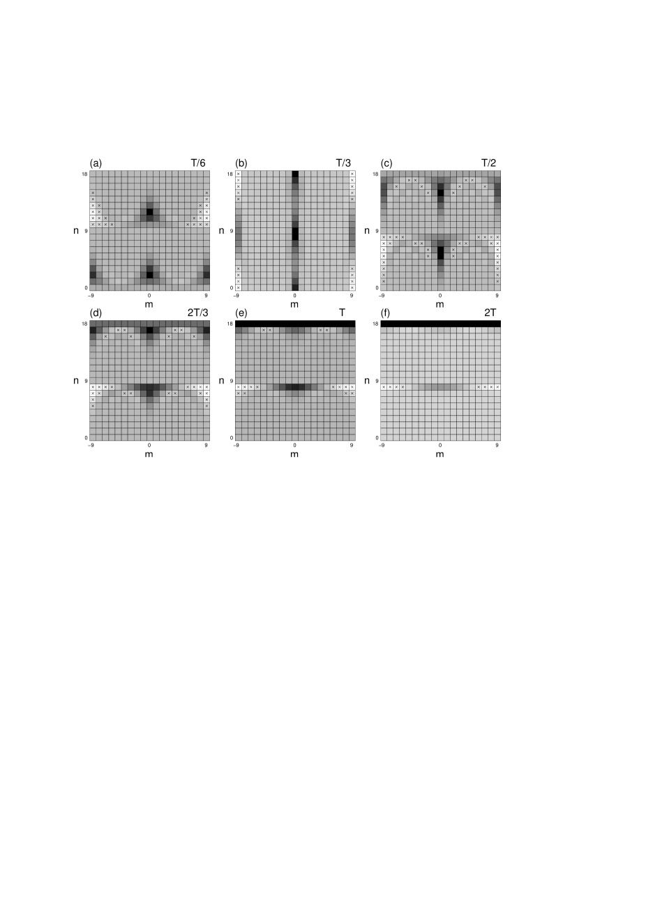
Fig. 1.6: Truncated coherent states: Wigner function for $|\overline{\alpha}\rangle_{(18)}$ with different displacement parameters $\overline{\alpha}$ given by fractions of $T=8.8$.

normalized by

$${\mathcal{}N}_{s} = \Big{(}\sum_{n=0}^{s}\frac{|{\overline{\alpha}\,}|^{2n}}{n!}\Big{)}^{-1/2}\;=\;\left\{(-1)^{s}{\mathrm{L}}^{-s-1}_{s}(|{\overline{\alpha}\,}|^{2})\right\}^{-1/2}$$ (1.38)

where ${\mathrm{L}}^{n}_{s}(x)$ is the generalized Laguerre polynomial. Equation (1.36) is just the Fock expansion of the conventional ID CS, which are truncated at an $s$th term and properly normalized. For this reason we shall refer to the state (1.36) as the truncated CS. In Fig. 1.5, the superposition coefficients $b_{n}^{(s)}$, given by Eq. (1.37) for the truncated CS $|{\overline{\alpha}\,}{\rangle\!_{(s)}}$ are presented as a function of the parameter $|{\overline{\alpha}\,}|\equiv|\alpha|$ in ${\mathcal{}H}^{(s)}$ with $s=1,2,3$ and $s=\infty$. As seen in Fig. 1.5, the coefficients $b^{(s)}_{n}$ are aperiodic functions of $|{\overline{\alpha}\,}|$. We emphasize the essential difference between the generalized and truncated CS. The former are periodic or quasiperiodic, while the latter are aperiodic in $|{\overline{\alpha}\,}|=|\alpha|$. Nevertheless, both $|\alpha{\rangle\!_{(s)}}$ and $|{\overline{\alpha}\,}{\rangle\!_{(s)}}$, go over into the conventional Glauber CS in the limit of $s\rightarrow\infty$ as is convincingly depicted in Fig. 1.3. By definition, the truncated CS go over into the Glauber CS in the limit of $s\rightarrow\infty$. Nevertheless, for better comparison with the generalized CS, given by (1.20), we show this property explicitly by expanding the scalar products between $|{\overline{\alpha}\,}{\rangle\!_{(s)}}$ and $|\alpha{\rangle\!_{(\infty)}}$ in power series of $|\alpha|$. We have [20]

$${{}_{(\infty)}\!\langle}\alpha|{\overline{\alpha}\,}{\rangle\!_{(1)}} = 1-{\textstyle\frac{1}{4}\,}|\alpha|^{4}+{\textstyle\frac{1}{6}\,}|\alpha|^{6}-{\mathcal{}O}(|\alpha|^{8})$$

$${{}_{(\infty)}\!\langle}\alpha|{\overline{\alpha}\,}{\rangle\!_{(2)}} = 1-{\textstyle\frac{1}{12}\,}|\alpha|^{6}+{\textstyle\frac{1}{16}\,}|\alpha|^{8}-{\mathcal{}O}(|\alpha|^{10})$$

$${{}_{(\infty)}\!\langle}\alpha|{\overline{\alpha}\,}{\rangle\!_{(3)}} = 1-{\textstyle\frac{1}{48}\,}|\alpha|^{8}+{\textstyle\frac{1}{60}\,}|\alpha|^{10}-{\mathcal{}O}(|\alpha|^{12})$$ (1.39)

where we put $\alpha={\overline{\alpha}\,}$. We find by induction that, with increasing dimension $(s+1)$, the truncated CS approach the conventional CS

$${{}_{(\infty)}\!\langle}\alpha|{\overline{\alpha}\,}{\rangle\!_{(s)}} = 1-\frac{|\alpha|^{2(s+1)}}{2\,(s+1)!}+{\mathcal{}O}(|\alpha|^{2(s+2)})$$ (1.40)

for $|\alpha|\equiv|{\overline{\alpha}\,}|^{2}\ll s$. Although Eqs. (1.28) and (1.40) have the same form, a closer comparison of Eqs. (1.27) and (1.39) shows that the states $|\alpha{\rangle\!_{(s)}}$ approach $|\alpha{\rangle\!_{(\infty)}}$ slower than $|{\overline{\alpha}\,}{\rangle\!_{(s)}}$ do and, in fact, the corrections ${\mathcal{}O}(|\alpha|^{2(s+2)})$ in Eq. (1.39) are smaller than those in Eq. (1.27). Finally, let us expand the scalar product between $|\alpha{\rangle\!_{(s)}}$ and $|{\overline{\alpha}\,}{\rangle\!_{(s)}}$ for $s$=1, 2, 3 in power series of $\alpha\equiv{\overline{\alpha}\,}$. We find that

$${{}_{(1)}\!\langle}\alpha|{\overline{\alpha}\,}{\rangle\!_{(1)}} = 1-{\textstyle\frac{1}{18}\,}|\alpha|^{6}+{\textstyle\frac{1}{15}\,}|\alpha|^{8}-{\mathcal{}O}(|\alpha|^{10})$$

$${{}_{(2)}\!\langle}\alpha|{\overline{\alpha}\,}{\rangle\!_{(2)}} = 1-{\textstyle\frac{1}{64}\,}|\alpha|^{8}+{\textstyle\frac{9}{800}\,}|\alpha|^{10}-{\mathcal{}O}(|\alpha|^{12})$$

$${{}_{(3)}\!\langle}\alpha|{\overline{\alpha}\,}{\rangle\!_{(3)}} = 1-{\textstyle\frac{1}{300}\,}|\alpha|^{10}+{\textstyle\frac{13}{5040}\,}|\alpha|^{12}-{\mathcal{}O}(|\alpha|^{14})$$ (1.41)

The expansions up to $|\alpha|^{2(s+2)}$ can be written in general form as

$${{}_{(s)}\!\langle}\alpha|{\overline{\alpha}\,}{\rangle\!_{(s)}} = 1-\frac{|\alpha|^{2(s+2)}}{2s!(s+2)^{2}}+{\mathcal{}O}(|\alpha|^{2(s+3)})$$ (1.42)

All these three types of CS are approximately equal for $|{\overline{\alpha}\,}|^{2}=|\alpha|^{2}\ll s$, since the scalar products between them tend to unity. The higher $s$, the greater is the range of $|\alpha|$, where the scalar product tends to unity. However, the states are significantly different for values $|\alpha|^{2}\approx s$. By comparing Eqs. (1.28), (1.40) and (1.42) for the same $s$, we observe that $|\alpha{\rangle\!_{(s)}}$ and $|{\overline{\alpha}\,}{\rangle\!_{(s)}}$ approach each other faster than $|\alpha{\rangle\!_{(\infty)}}$.

In order to calculate the Wigner function, we substitute Eq. (1.37) into Eq. (1.17), arriving at

$$W_{s}(n,\theta_{m}) = \frac{{\mathcal{}N}_{s}^{2}}{s+1}\left(\sum_{k=0}^{M}\frac{|{\overline{\alpha}\,}|^{M}}{\sqrt{k!(M-k)!}}\exp[{\mathrm{i}}(2k-M)(\theta_{m}-\varphi)]\right.$$ (1.43)

$$\qquad+\left.\sum_{k=M+1}^{s}\frac{|{\overline{\alpha}\,}|^{M+s+1}}{\sqrt{k!(M-k+s+1)!}}\right)$$

where $M=2n\ \mbox{mod}(s+1)$. Equation (1.43) can be written in a form useful for a comparison with the Vaccaro–Pegg result

$$W_{s}(n,\theta_{m})=\frac{1}{s+1}\Big{[}\Lambda_{1}(n,|{\overline{\alpha}\,}|)\Phi_{1}(n,\theta_{m},\varphi)+\Lambda_{2}(n,|{\overline{\alpha}\,}|)\Phi_{2}(n,\theta_{m},\varphi)\Big{]}$$ (1.44)

where

$$\Lambda_{1}(n,|{\overline{\alpha}\,}|) = \frac{{\mathcal{}N}_{s}^{2}|{\overline{\alpha}\,}|^{M}}{\mu_{1}!}$$

$$\Phi_{1}(n,\theta_{m},\varphi) = \mu_{1}!\sum_{k=0}^{M}\frac{\cos[(2k-M)(\theta_{m}-\varphi)]}{[k!(M-k)!]^{1/2}}$$ (1.45)

and

$$\Lambda_{2}(n,|{\overline{\alpha}\,}|) = \frac{{\mathcal{}N}_{s}^{2}|{\overline{\alpha}\,}|^{M+s+1}}{\mu_{2}!}$$

$$\Phi_{2}(n,\theta_{m},\varphi) = \mu_{2}!\sum_{k=M+1}^{s}\frac{\cos[(2k-M-s-1)(\theta_{m}-\varphi)]}{[k!(M-k+s+1)!]^{1/2}}$$ (1.46)

Here, $\mu_{1}=[\![M/2]\!]$ is the integer part of $M/2$, and similarly $\mu_{2}=[\![(M+1+s)/2]\!]$. We note that the functions $\Lambda_{i}$ do not depend on the phase $\varphi$ of ${\overline{\alpha}\,}$ and similarly the functions $\Phi_{i}$ do not depend on its amplitude $|{\overline{\alpha}\,}|$. In the Vaccaro–Pegg treatment, $|{\overline{\alpha}\,}|^{2}$ was always much less than $s$, so that the second term of Eq. (1.44) could be neglected. Then the Wigner function was factorizable into the amplitude dependent function $\Lambda_{1}$ and the phase dependent function $\Phi_{1}$, and the normalizing constant ${\mathcal{}N}_{s}$ was approximated by $\exp(-|{\overline{\alpha}\,}|^{2}/2)$. It can be seen that for general values of ${\overline{\alpha}\,}$ of the truncated CS this factorization is no longer feasible. Moreover, for large $|{\overline{\alpha}\,}|$, the second term of Eq. (1.44) becomes predominant. We compare different shapes of the $W$ functions for various ${\overline{\alpha}\,}$ in Fig. 1.6. The functions are computed for $s=18$. With $|\alpha|$ increasing from zero, the shape of the generalized CS is initially very similar to that of the truncated CS (see Fig. 1.4). It occurs up to the peak–antipeak transition from $n=s$ to $n=0$ around the value $|{\overline{\alpha}\,}|^{2}\approx s/2$ (corresponding to $|\alpha|\approx T_{s}/3$ in Fig. 1.6b). However, if $|{\overline{\alpha}\,}|^{2}\gg s/2$, the situation is inverse: the second term of Eq. (1.44) is now predominant and we observe two peaks for $n>s/2$ and a peak — antipeak structure for $n\leq s/2$ (for instance, Fig. 1.6d). In the case when $|{\overline{\alpha}\,}|^{2}\approx s$ (Fig. 1.6c), the $W$ function has a more general shape. With increasing $|{\overline{\alpha}\,}|$ the two-peak structure shifts to larger values of $n$, while the peak–antipeak structure gradually vanishes at $n\leq s/2$ (Fig. 1.6d–e). The shape is still comparatively simple because the function Eq. (1.44) is a sum of only two factorizable terms. By further increasing $|{\overline{\alpha}\,}|\gg T_{s}$, the Wigner function has a very simply structure representing the number state $|s\rangle$. Even for $|{\overline{\alpha}\,}|=2T_{s}$, as presented in Fig. 1.6f, the peak–antipeak structure at $n\leq s/2$ vanishes almost completely. In the limit of $|{\overline{\alpha}\,}|^{2}/s\rightarrow\infty$, the truncated CS approaches the number state $|s\rangle$. This conclusion can also be deduced from the behavior of the superposition coefficients $b^{(s)}_{n}$ in their dependence on $|{\overline{\alpha}\,}|$ as depicted Fig. 1.5. In contrast to the generalized CS, the behavior of the truncated CS is aperiodic in $|{\overline{\alpha}\,}|$.

C.   Example: Two-dimensional Coherent States

The simplest nontrivial FD states are those spanned in a two-dimensional system, namely, for $s=1$. States in such a system have intensively been studied by authors dealing with the general problem of finite-dimensional quantum-optical states [16, 17, 28]. Here, we would like to discuss this problem from other points of view. Two-dimensional systems are well known in various fields of physics, and we thus can apply the results and concepts to describe our situation. Examples of realizations of such a system can be given by the spin projection of spin-$\frac{1}{2}$ particle, two-level atom or quantum dot. Hence, the CS in ${\mathcal{}H}^{(1)}$ [see Eqs. (1.50) and (1.52)] can, in fact, be identified with the coherent spin-$\frac{1}{2}$ state [4] or equivalently with the two-level atomic coherent state [5]. In the case of $s$=1, the terms photon number, phase and FD harmonic oscillator are a bit confusing and should be understood, for example, as [55]: $z$ component of spin divided by $\hbar$, angle of orientation about the $z$ axis and spin, respectively, or equivalently as atomic quantities [5, 16]. We use the notion two-dimensional space or states to be consistent with our general terminology applied in earlier sections. Although, we are aware that this terminology might be misleading. In this section we use a Poincaré sphere representation for the description of the states discussed and their properties, like various operator averages and squeezing degrees. Finally, we present the $W$ function for two-dimensional CS.

It is well known that states in a two-dimensional system can be described by means of the Stokes parameters and visualized by means of the Poincaré sphere. The density matrix of any two-state system can be written in the form

$$\hat{\rho} = \frac{1}{2}\left(\begin{array}[]{cc}1+{\mathcal{}S}_{z}&{\mathcal{}S}_{x}+{\mathrm{i}}{\mathcal{}S}_{y}\\ {\mathcal{}S}_{x}-{\mathrm{i}}{\mathcal{}S}_{y}&1-{\mathcal{}S}_{z}\end{array}\right)$$ (1.49)

where ${\mathcal{}S}_{x},\ {\mathcal{}S}_{y}$, and ${\mathcal{}S}_{z}$ are the Stokes parameters. Using these parameters as coordinates of a point in three-dimensional space, any state corresponds to a point on a unit radius sphere, the so-called Poincaré sphere. Pure states are represented by points on the surface, while mixed-state points lie inside the sphere. Now, using this tool, we can display both the two-dimensional generalized and truncated CS and compare their expressions.

For the two-dimensional generalized CS, given by

$$\,|\alpha{\rangle\!_{(1)}}=\cos|\alpha||0\rangle+\exp({\mathrm{i}}\varphi)\sin|\alpha|\,|1\rangle$$ (1.50)

the Stokes parameters are found to be

$${\mathcal{}S}_{x} = \sin 2|\alpha|\cos\varphi$$

$${\mathcal{}S}_{y} = -\sin 2|\alpha|\sin\varphi$$

$${\mathcal{}S}_{z} = \cos 2|\alpha|$$ (1.51)

We note that any pure state in ${\mathcal{}H}^{(1)}$ is coherent. The interpretation of the parameter $\alpha$ is very simple; its module is proportional to the polar coordinate, while its argument $\varphi$ is the azimuthal coordinate of the representative Poincaré sphere point.

Similarly, we find the Stokes parameters for the truncated CS, given by (1.36). The two-dimensional state $|{\overline{\alpha}\,}{\rangle\!_{(1)}}$, with the parameter ${\overline{\alpha}\,}=|{\overline{\alpha}\,}|\exp({\mathrm{i}}\varphi)$, is expressed by

$$|{\overline{\alpha}\,}{\rangle\!_{(1)}} = \frac{1}{\sqrt{1+|{\overline{\alpha}\,}|^{2}}}\,|0\rangle+\exp({\mathrm{i}}\varphi)\frac{|{\overline{\alpha}\,}|}{\sqrt{1+|{\overline{\alpha}\,}|^{2}}}\,|1\rangle$$ (1.52)

$$= \cos(\arctan|{\overline{\alpha}\,}|)|0\rangle+\exp({\mathrm{i}}\varphi)\sin(\arctan|{\overline{\alpha}\,}|)\,|1\rangle$$

The Stokes parameters are now

$${\mathcal{}S}_{x} = 2\frac{|{\overline{\alpha}\,}|}{1+|{\overline{\alpha}\,}|^{2}}\cos\varphi$$

$${\mathcal{}S}_{y} = -2\frac{|{\overline{\alpha}\,}|}{1+|{\overline{\alpha}\,}|^{2}}\sin\varphi$$

$${\mathcal{}S}_{z} = \frac{1-|{\overline{\alpha}\,}|^{2}}{1+|{\overline{\alpha}\,}|^{2}}$$ (1.53)

The function of the argument $\varphi$ is the same as for the generalized CS, while the meaning of the module $|{\overline{\alpha}\,}|$ is different from that of $|\alpha|$. We observe, for instance, neither periodicity nor quasiperiodicity in $|{\overline{\alpha}\,}|$. To interpret $|{\overline{\alpha}\,}|$, we write the last equation in (1.53) in the form $|{\overline{\alpha}\,}|/(1-{\mathcal{}S}_{z}^{2})^{1/2}=1/(1+{\mathcal{}S}_{z})$. Thus, for a given ${\overline{\alpha}\,}$, one can construct the corresponding Poincaré sphere point as follows [20]: (1) by locating the complex number ${\overline{\alpha}\,}$ in the ${\mathcal{}S}_{x}{\mathcal{}S}_{y}$ plane, so that the ${\mathcal{}S}_{x}$ ($-{\mathcal{}S}_{y}$) coordinate is the real (imaginary) part of ${\overline{\alpha}\,}$, respectively; and (2) by connecting this point with the lower pole of the Poincaré sphere by a straight line. The other intersection of the line and the sphere is then the point representing the coherent state.

For the case of two-dimensional CS, there have been computed quantities such as the mean values and variances of the various operators, including $\hat{N}$ and $\hat{\Phi}$ quadratures, and their commutators [16, 17]. Most of these quantities can easily be displayed on the Poincaré sphere and expressed by means of the Stokes parameters. We find that the following mean values and variances are given respectively by

$$\langle{\hat{N}}\rangle = \frac{1-{\mathcal{}S}_{z}}{2}$$

$$\langle(\Delta{\hat{N}})^{2}\rangle = \frac{{\mathcal{}S}_{x}^{2}+{\mathcal{}S}_{y}^{2}}{4}$$

$$\langle{\hat{\Phi}}\rangle = \frac{(1-{\mathcal{}S}_{x})\pi}{2}$$

$$\langle(\Delta{\hat{\Phi}})^{2}\rangle = \frac{{\mathcal{}S}_{y}^{2}+{\mathcal{}S}_{z}^{2})\pi^{2}}{4}$$ (1.54)

and the mean value of the $\hat{N}-\hat{\Phi}$ commutator is

$$\langle[\hat{N},\hat{\Phi}]\rangle = \frac{{\mathrm{i}}\pi{\mathcal{}S}_{y}}{2}$$ (1.55)

The degrees of squeezing $S_{N}$ and $S_{\Phi}$ are defined by

$$S_{N} = 2\langle(\Delta{\hat{N}})^{2}\rangle\,|\langle[\hat{N},\hat{\Phi}]\rangle|^{-1}-1$$

$$S_{\Phi} = 2\langle(\Delta{\hat{\Phi}})^{2}\rangle\,|\langle[\hat{N},\hat{\Phi}]\rangle|^{-1}-1$$ (1.56)

They can be written in terms of the Stokes parameters as

$$S_{N} = \frac{1}{\pi}\frac{{\mathcal{}S}_{x}^{2}+{\mathcal{}S}_{y}^{2}}{|{\mathcal{}S}_{y}|}-1$$

$$S_{\Phi} = \pi\frac{{\mathcal{}S}_{y}^{2}+{\mathcal{}S}_{z}^{2}}{|{\mathcal{}S}_{y}|}-1$$ (1.57)

We found for the case of $s=1$ that the averages of the quantum-optical quantities are simply related to the Stokes parameters. The correspondence can also be expressed in terms of the operators $\hat{N}$ and $\hat{\Phi}$ in relation to the Pauli matrices $\hat{\sigma}_{z}$ and $\hat{\sigma}_{x}$, or the quadratures $\hat{X}_{a}$ and $\hat{Y}_{a}$ related to $\hat{\sigma}_{x}$ and $\hat{\sigma}_{y}$.

Finally, we find the explicit expression for the Wigner function in $n$ and $\theta$ for two-dimensional generalized CS. We get

$$W_{s}(n,\theta_{m}) = {\textstyle\frac{1}{4}\,}\Bigl{[}1+(-1)^{n}\cos(2|\alpha|)$$ (1.58)

$$+\;(-1)^{m}\sqrt{2}\sin(2|\alpha|)\cos\Bigl{(}\varphi-(-1)^{n}{\textstyle\frac{\pi}{4}\,}\Bigr{)}\Bigr{]}$$

On simple replacement of $|\alpha|$ by $\arctan|{\overline{\alpha}\,}|$ in Eq. (1.58), one obtains the $W$ function for the two-dimensional truncated CS.

V.   OTHER FD QUANTUM-OPTICAL STATES

Analogously to the generalized CS in a FD Hilbert space, analyzed in Section IV.A, other states of the electromagnetic field can be defined by the action of the FD displacement or squeeze operators. In particular, FD displaced phase states and coherent phase states were discussed by Gangopadhyay [28]. Generalized displaced number states and Schrödinger cats were analyzed in Ref. [21] and generalized squeezed vacuum was studied in Ref. [34]. A different approach to construction of FD states can be based on truncation of the Fock expansion of the well-known ID harmonic oscillator states. The same construction, as for the truncated CS, was applied to analyze, for instance, truncated Schrödinger cats by Zhu and Kuang [25, 35], Miranowicz et al. [21], and Roy and Roy [24]; truncated phase CS by Kuang and Chen [27]; truncated displaced number states by Miranowicz, et al. [21], or truncated squeezed vacuum by Miranowicz et al. [34].

A.   FD Phase Coherent States

Here, we study two kinds of FD phase coherent states associated with the Pegg–Barnett Hermitian optical phase formalism [26]. First states, referred to as the generalized phase CS or coherent phase states, are generated by the action of the phase displacement operator. This definition of the phase CS was applied by Gangopadhyay [28] in close analogy to Glauber’s idea of the conventional CS. The second definition of phase CS is based on another phase “displacement” operator formally designed by Kuang and Chen [27]. We shall refer to these states as the truncated phase CS to stress its similarity to the truncated CS described in Section IV.B. We construct the phase CS explicitly and derive their discrete Wigner representation. The FD phase CS are not only mathematical structures. A framework for their physical interpretation is provided by cavity quantum electrodynamics and atomic physics.

1. Generalized Phase CS

Gangopadhyay [28] has proposed a definition of the generalized phase CS in formal analogy to the generalized CS, defined by Eq. (1.20). The main idea is to choose a preferred phase state $|\theta_{0}\rangle$, and then to construct the phase creation ($\hat{\phi}_{s}^{\dagger}$) and phase annihilation ($\hat{\phi}_{s}$) operators analogously to the conventional (photon-number) creation and annihilation operators. The phase CS are then constructed by replacing vacuum $|0\rangle$ by $|\theta_{0}\rangle$, and the operators $\hat{a}_{s}$ and $\hat{a}_{s}^{\dagger}$ by $\hat{\phi}_{s}$ and $\hat{\phi}_{s}^{\dagger}$, respectively, as given by Eq. (1.11). Thus, the generalized phase CS is defined to be [28]

$$|\beta,\theta_{0}{\rangle\!_{(s)}}=\hat{D}_{s}(\beta,\theta_{0})\,|\theta_{0}\rangle$$ (1.59)

by the action of the phase displacement operator

$$\hat{D}^{(s)}(\beta,\theta_{0})=\exp[\beta\hat{\phi}_{s}^{\dagger}-\beta^{*}\hat{\phi}_{s}]$$ (1.60)

on the preferred phase state $|\theta_{0}\rangle$. By generalizing the method described in Appendix, one can find the following phase-state representation of the generalized phase CS [29]

$$|\beta,\theta_{0}{\rangle\!_{(s)}} = \sum_{m=0}^{s}{\mathrm{e}}^{{\mathrm{i}}(\mu-m_{0})\varphi}\,b_{m}^{(s)}|\theta_{m}\rangle$$ (1.61)

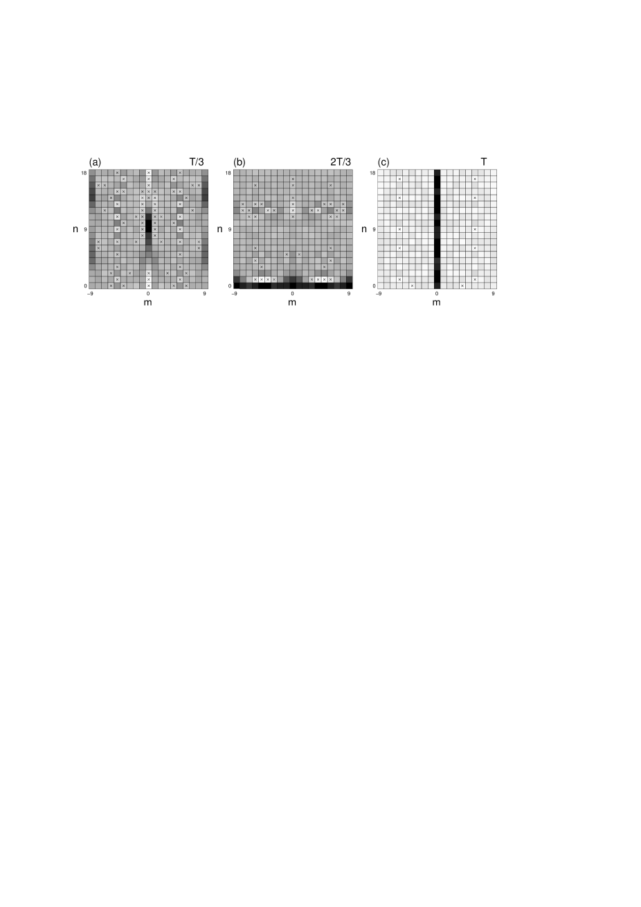
Fig. 1.7: Generalized phase coherent states: Wigner function for $|\beta,0\rangle_{(18)}$ with different phase-displacement parameters $\beta$ chosen to be fractions of the quasiperiod $T=T_{18}=8.8$.

where $\varphi={\mathrm{A}rg}\beta$ and the decomposition coefficients are

$$b_{m}^{(s)}\;\equiv\;b_{m}^{(s)}(\theta_{0}) = \frac{s!}{s+1}(-1)^{m+m_{0}}\,\frac{{\mathrm{i}}^{m_{0}+\mu}}{\sqrt{\mu!m_{0}!}}$$ (1.62)

$$\times\sum_{k=0}^{s}\exp\left({\mathrm{i}}x_{k}\gamma_{s}|\beta|\right)\frac{{\mathrm{H}e}_{\mu}(x_{k}){\mathrm{H}e}_{m_{0}}(x_{k})}{{\mathrm{H}e}_{s}^{2}(x_{k})}$$

Here, $x_{l}\equiv x_{l}^{(s+1)}$ are the roots of the Hermite polynomial, $\mbox{He}_{s+1}(x_{l})=0$. For brevity, we have denoted $\mu=m+m_{0}\ \mbox{mod}(s+1)$ and $\gamma_{s}=\sqrt{\frac{2\pi}{s+1}}$. The values $\theta_{m}$ are chosen $\mbox{mod}(2\pi)$. We also assume that the permitted values of $\theta_{0}$ are not completely arbitrary but restricted to $\frac{2\pi}{s+1}m_{0}\ \mbox{mod}(2\pi)$ (where $m_{0}=0,1,\dots$). In a special case, for $\theta_{0}=0$ and $s=1$, the phase CS reduce to the state $|\beta,\theta_{0}=0{\rangle\!_{(1)}}$ studied by Gangopadhyay [28]. Here, for simplicity, we also consider the case of $\theta_{0}=0$.

2. Truncated Phase CS

Kuang and Chen [27] defined the FD phase CS, denoted as $|{\overline{\beta}\,},\theta_{0}{\rangle\!_{(s)}}$, by the action of the FD operator $\exp({\overline{\beta}}\hat{\phi}_{s}^{\dagger})$ on the phase state $|\theta_{0}\rangle$. The reference phase $\theta_{0}$ is chosen as zero [27]. Therefore, on comparing the explicit expressions for $\hat{a}_{s}$ and $\hat{\phi}_{s}$, it is clear that the states $|{\overline{\beta}\,},\theta_{0}{\rangle\!_{(s)}}$ are in close analogy to the truncated CS [20]. For this reason we shall refer to the states $|{\overline{\beta}\,},\theta_{0}{\rangle\!_{(s)}}$ as the truncated phase CS in ${\mathcal{}H}^{(s)}$. For completeness, we present the phase-space expansion with ${\overline{\beta}}=|{\overline{\beta}}|\exp({\mathrm{i}}\varphi)$ given by [27]

$$|{\overline{\beta}},\theta_{0}{\rangle\!_{(s)}} = {\mathcal{}N}_{s}\exp({\overline{\beta}}\hat{\phi}_{s}^{\dagger})|\theta_{0}\rangle\;=\;\sum_{m=0}^{s}{\mathrm{e}}^{{\mathrm{i}}m\varphi}\,b_{m}^{(s)}|\theta_{m}\rangle$$ (1.63)

where

$$b_{m}^{(s)}={\mathcal{}N}_{s}\frac{(\gamma_{s}|{\overline{\beta}}|)^{m}}{\sqrt{m!}},\qquad{\mathcal{}N}_{s}=\left(\sum_{n=0}^{s}\frac{(\gamma_{s}|{\overline{\beta}}|)^{2n}}{n!}\right)^{-1/2}$$ (1.64)

and $\gamma_{s}=\sqrt{\frac{2\pi}{s+1}}$ as in Eq. (1.62). In particular, squeezing properties of the truncated phase CS were analyzed by Kuang and Chen [27]. They have paid special attention to the two-dimensional case.

Although many properties of the phase CS are known by now, for their better understanding it is very useful to analyze graphs of their quasidistributions. The discrete Wigner function, as defined by Wootters [55] (see also Ref. [57]), takes the following form for $s>1$

$$W_{s}(n,\theta_{m}) = \frac{1}{s+1}\sum_{p=0}^{s}b^{(s)}_{m+p}\,b^{(s)}_{m-p}\exp\left[-2{\mathrm{i}}p\left(\frac{2\pi}{s+1}n+\varphi\right)\right]$$ (1.65)

for the generalized phase CS with $b^{(s)}_{n}$ given by (1.62) and for the truncated phase CS with superposition coefficients (1.64). In Eq. (1.65), the subscripts $m\pm p$ are assumed to be $\mbox{mod}(s+1)$. One can obtain the particularly simple Wigner function for $s=1$ [55].

The generalized phase CS, $|\beta,\theta_{0}{\rangle\!_{(s)}}$, and truncated phase CS, $|{\overline{\beta}\,},\theta_{0}{\rangle\!_{(s)}}$, are associated with the Pegg–Barnett formalism of the Hermitian phase operator ${\hat{\Phi}_{s}}$. The operators ${\hat{\Phi}_{s}}$, $\hat{\phi}_{s}$, and $\hat{\phi}_{s}^{\dagger}$ do not exist in the conventional ID Hilbert space ${\mathcal{}H}^{(\infty)}$. Thus the generalized and truncated phase CS are properly defined only in ${\mathcal{}H}^{(s)}$ of finite dimension. States $|\beta,\theta_{0}{\rangle\!_{(s)}}$ and $|{\overline{\beta}\,},\theta_{0}{\rangle\!_{(s)}}$, similarly to $|\alpha{\rangle\!_{(s)}}$ and $|\overline{\alpha}{\rangle\!_{(s)}}$, approach each other for $|\beta|^{2}=|{\overline{\beta}}|^{2}\ll s/\pi$ [20]. This can be shown explicitly by calculating the scalar product between generalized and truncated phase CS. We find ($\beta={\overline{\beta}}$)

$${{}_{(s)}\!\langle}\beta,\theta_{0}|{\overline{\beta}},\theta_{0}{\rangle\!_{(s)}} = 1-\frac{(\sqrt{\pi}|\beta|)^{2(s+2)}}{2s!(s+2)^{2}}+{\mathcal{}O}(|\beta|^{2(s+3)})$$ (1.66)

For values $|\beta|^{2}=|{\overline{\beta}}|^{2}\approx s/\pi$ or greater than $s/\pi$, the differences between $|\beta,\theta_{0}{\rangle\!_{(s)}}$ and $|{\overline{\beta}\,},\theta_{0}{\rangle\!_{(s)}}$ become significant.

In Fig. 1.7, a few examples of the Wigner function for $|\beta,0{\rangle\!_{(18)}}$ are presented for different values of the phase displacement parameter $\beta$. Because of space limits in this chapter, the corresponding figures for the truncated phase CS are not presented. In Fig. 1.7c, we observe that $|\beta,0{\rangle\!_{(s)}}$ is quasiperiodic in $\beta$. Closer analysis of Eq. (1.62), in comparison to (1.23), shows that the quasiperiod $T_{s}$ for $|\beta,0{\rangle\!_{(s)}}$ is the same as that for the generalized coherent states. Thus, it is given by Eq. (1.34) for even $s$ and Eq. (1.35) for odd $s$. Yet, the evolution of the generalized phase CS is more complicated than that for the generalized CS, as seen on comparing Figs. 1.7a,b with the corresponding Figs. 1.4b,d. As was discussed in Ref. [29], the truncated phase CS are aperiodic in ${\overline{\beta}}$ for any dimension.

B.   FD Displaced Number States

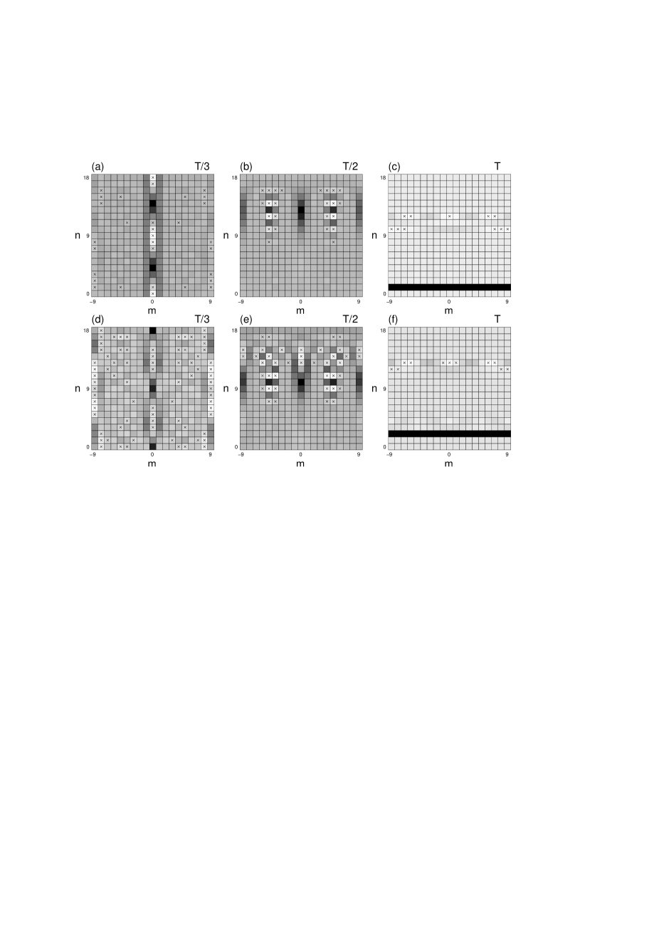
Fig. 1.8: Generalized displaced number states: Wigner function for $|\alpha,n_{d}\rangle_{(s)}=|\alpha,1\rangle_{(18)}$ (a–c) and $|\alpha,2\rangle_{(18)}$ (d–f) with different displacement parameters $\alpha$ given by fractions of the quasiperiod $T=T_{18}=8.8$.

In this section, we propose two nonequivalent definitions of the displaced number states (DNS) in the FD Hilbert space and show that the FD states go over into the conventional DNS discussed, for instance, by de Oliveira et al. [65].

1. Generalized DNS

Analogously to the generalized CS, given by Eq. (1.20), we define the generalized DNS as follows

$$|\alpha,n_{d}{\rangle\!_{(s)}}={\hat{D}}^{(s)}(\alpha)|n_{d}\rangle$$ (1.67)

as the result of action of the displacement operator ${\hat{D}}^{(s)}(\alpha)$, given by Eq. (1.21), on the number state $|n_{d}\rangle$. By using the same method as described in Appendix for $|\alpha\rangle{\!{}_{(s)}}$, we find the following explicit Fock representation of the generalized DNS

$$|\alpha,n_{d}{\rangle\!_{(s)}}={\hat{D}}_{s}(\alpha)|n_{d}\rangle=\sum_{n=0}^{s}{\mathrm{e}}^{{\mathrm{i}}(n-n_{d})\varphi}\,b^{(s)}_{n}|n\rangle$$ (1.68)

where

$$b^{(s)}_{n}\;\equiv\;b^{(s)}_{n}(n_{d})=\frac{s!}{s+1}\ \frac{\,{\mathrm{i}}^{n_{d}}(-{\mathrm{i}})^{n}}{\sqrt{n!n_{d}!}}\sum_{k=0}^{s}{\mathrm{e}}^{{\mathrm{i}}x_{k}|\alpha|}\,\frac{{\mathrm{H}e}_{n}(x_{k}){\mathrm{H}e}_{n_{d}}(x_{k})}{{\mathrm{H}e}_{s}^{2}(x_{k})}$$ (1.69)

and $\alpha=|\alpha|{\exp({\mathrm{i}}\varphi)}$. In the dimension limit, $s\rightarrow\infty$, the generalized DNS go over into the conventional DNS defined, for instance, in Refs. [65, 43]. This property can readily be deduced from $\lim_{s\rightarrow\infty}\hat{D}_{s}=\hat{D}_{\infty}\equiv\hat{D}$. Obviously, in the special case of $n_{d}=0$ the generalized DNS reduce to the generalized CS defined by Eq. (1.20).

2. Truncated DNS

Let us define the finite-dimensional DNS, which in a special case go over into the truncated CS of Kuang et al. [17] and into the conventional DNS [65] in the limit of $s\rightarrow\infty$. We define the truncated displaced number states, $|{\overline{\alpha}},n_{d}{\rangle\!_{(s)}}$, by the following Fock representation

$$|{\overline{\alpha},n_{d}\rangle}{\!{}_{(s)}}=\sum_{n=0}^{s}b^{(s)}_{n}{\mathrm{e}}^{{\mathrm{i}}(n-n_{d})\varphi}|n\rangle$$ (1.70)

where

$$b^{(s)}_{n}\;\equiv\;b^{(s)}_{n}(n_{d})={\mathcal{}N}_{s}\left(\frac{n_{1}!}{n_{2}!}\right)^{1/2}\,(-1)^{n_{2}-n}\,|{\overline{\alpha}\,}|^{n_{2}-n_{1}}L_{n_{1}}^{n_{2}-n_{1}}(|{\overline{\alpha}\,}|^{2})$$ (1.71)

$${\mathcal{}N}_{s}\equiv{\mathcal{}N}_{s}(|\overline{\alpha}|,n_{d})=\left(\sum_{n=0}^{s}\frac{n_{1}!}{n_{2}!}\,|\overline{\alpha}|^{2(n_{2}-n_{1})}\left[L_{n_{1}}^{n_{2}-n_{1}}(|\overline{\alpha}|^{2})\right]^{2}\right)^{-1/2}$$ (1.72)

For brevity, we have introduced the indices $n_{1}\equiv\min(n,n_{d})$ and $n_{2}\equiv\max(n,n_{d})$. The state (1.70) is, in fact, given by the Fock expansion of the conventional ID DNS [65, 43], which are truncated at the $(s+1)$th term and properly normalized. This construction justifies our name for Eq. (1.70). Alternatively, the states (1.70) can be defined by the action of the FD factorized displacement operator, $\exp({\overline{\alpha}\,}{\ \hat{a}_{s}}^{\dagger})\exp(-{\overline{\alpha}\,}^{*}{\hat{a}_{s}})$, on a number state $|n_{d}\rangle$:

$$|{\overline{\alpha},n_{d}\rangle}{\!{}_{(s)}}={\mathcal{}N}_{s}\exp(\overline{\alpha}{\hat{a}_{s}}^{\dagger})\exp({-\overline{\alpha}}^{*}\hat{a}_{s})|n_{d}\rangle$$ (1.73)

This equation explicitly shows how the concept of the truncated CS, given by (1.36), is generalized. The truncated DNS are different from the generalized DNS, given by (1.67). The differences are particularly distinct for values $|{\overline{\alpha}\,}|^{2}\equiv|\alpha|^{2}$ of the order $s$ or greater. However, for $|{\overline{\alpha}}|^{2}\equiv|\alpha|^{2}\ll s,$ the FD displaced number states $|\alpha,n_{d}{\rangle\!_{(s)}}$ and $|{\overline{\alpha}\,},n_{d}{\rangle\!_{(s)}}$ approach each other.

In Fig. 1.8, we present a few examples of the Wigner function for the generalized DNS with $n_{d}$=1, and 2. We observe that $|\alpha,n_{d}\rangle{\!{}_{(s)}}$ are quasiperiodic in $|\alpha|$ with the same quasiperiods as those for the generalized CS given by Eqs. (1.34) and (1.35) for even and odd $s$, respectively. At multiples of $T_{s}$, the initial number state $|n_{d}\rangle$ is partially recovered, as observed in Figs. 1.4f and 1.8c,f. However, the periodicity is deteriorated with increasing photon number $n_{d}$. The most precise periodicity is observed for $|\alpha,0\rangle{\!{}_{(s)}}$, as depicted in Fig. 1.4f. It is worse for $|\alpha,1\rangle{\!{}_{(s)}}$ (Fig. 1.8c), and even worse for $|\alpha,2\rangle{\!{}_{(s)}}$ as seen in Fig. 1.8f. In fact, the entire evolution of $|\alpha,n_{d}\rangle{\!{}_{(s)}}$ becomes more complicated with increasing number $n_{d}$ as can be observed by comparing Figs. 1.4b,c,f, 1.8a–c and 1.8d–f, respectively. For brevity, we omit the corresponding figures for the truncated DNS. The Wigner functions for $|\alpha,n_{d}{\rangle\!_{(s)}}$ and $|{\overline{\alpha}\,},n_{d}{\rangle\!_{(s)}}$ are almost indistinguishable for the displacement parameter $|\alpha|=|\overline{\alpha}|$ and $n_{d}$ much less than $s$. However, for higher values of these parameters, the generalized and truncated DNS behave qualitatively different. As discussed, the former states are periodic or quasiperiodic, but the latter are aperiodic with the increasing displacement parameter.

C.   FD Schrödinger Cats

Superpositions of two CS have attracted much attention [13, 66] as simple examples of Schrödinger cats. In this section, we will discuss two kinds of FD analogs of the conventional ID even and odd CS of Malkin and Man’ko [13]. The Schrödinger cats in FD Hilbert spaces were discussed, for example, by Zhu and Kuang [25], Miranowicz et al. [21], and Roy and Roy [24].

1. Generalized Schrödinger Cats

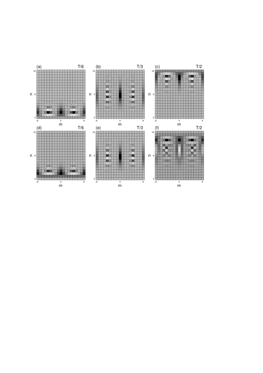
Fig. 1.9: Generalized Schrödinger cats: Wigner function for $|\alpha_{0}\rangle_{(18)}$ (a–c) and $|\alpha_{1}\rangle_{(18)}$ (d–f) with $\alpha$ given by fractions of the quasiperiod $T=T_{18}=8.8$.

Let us define the generalized even CS by [21]

$$|\alpha_{0}{\rangle\!_{(s)}}={\mathcal{}M}_{0s}\,\left(|\alpha{\rangle\!_{(s)}}+|-\alpha{\rangle\!_{(s)}}\right)$$ (1.74)

and odd CS by

$$|\alpha_{1}{\rangle\!_{(s)}}={\mathcal{}M}_{1s}\,\left(|\alpha{\rangle\!_{(s)}}-|-\alpha{\rangle\!_{(s)}}\right)$$ (1.75)

where the normalization is guaranteed by ${\mathcal{}M}_{\delta s}$ ($\delta=0,1$). On inserting Eq. (1.22) into (1.74) and (1.75), we find the Fock expansions of the Schrödinger cats in the forms

$$|\alpha_{0}{\rangle\!_{(s)}} = {\mathcal{}N}_{0s}\sum_{n=0}^{[\![s/2]\!]}{\mathrm{e}}^{{\mathrm{i}}2n\varphi}\,b_{2n}^{(s)}|2n\rangle$$

$$|\alpha_{1}{\rangle\!_{(s)}} = {\mathcal{}N}_{1s}\sum_{n=0}^{[\![s/2]\!]}{\mathrm{e}}^{{\mathrm{i}}(2n+1)\varphi}\,b_{2n+1}^{(s)}|2n+1\rangle$$ (1.76)

where the coefficients $b^{(s)}_{n}$ are given by Eq. (1.23); $[\![s/2]\!]$ is the integer part of $s/2$, and the normalizations are ($\delta=0,1$)

$${\mathcal{}N}_{\delta s}=\left(\sum_{n=0}^{[\![s/2]\!]}\big{(}b^{(s)}_{2n+\delta})^{2}\right)^{-1/2}$$ (1.77)

Analogously one can construct FD superpositions of several CS, that is FD Schrödinger cat-like or kitten states, which in the limit go over into the conventional ID ones [66, 67].

2. Truncated Schrödinger Cats

FD even and odd CS can be constructed in a way slightly different from that presented in the preceding paragraph. Instead of the generalized CS, the truncated CS can be used in the definitions (1.74) and (1.75). This approach was explored by Zhu and Kuang [25], and Roy and Roy [24]. We rewrite briefly their explicit expressions for $|{\overline{\alpha}\,}_{0}{\rangle\!_{(s)}}$ and $|{\overline{\alpha}\,}_{1}{\rangle\!_{(s)}}$ in Fock representation

$$|{{\overline{\alpha}\,}_{\delta}\rangle}{\!{}_{(s)}}={\mathcal{}N}_{\delta s}\sum_{n=0}^{[\![s/2]\!]}\frac{{{\overline{\alpha}\,}}^{2n+\delta}}{\sqrt{(2n+\delta)!}}|2n+\delta\rangle$$ (1.78)

where $\delta=0$ for even cats and $\delta=1$ for odd cats. The normalization is

$${\mathcal{}N}_{\delta s}=\left(\sum_{n=0}^{[\![s/2]\!]}\frac{|{{\overline{\alpha}\,}}|^{2(2n+\delta)}}{(2n+\delta)!}\right)^{-1/2}$$ (1.79)

Equation (1.78) can directly be calculated from Eqs. (1.74) and (1.75) after replacing $|\pm{\alpha}{\rangle\!_{(s)}}$ by $|\pm{{\overline{\alpha}\,}}{\rangle\!_{(s)}}$, given by their Fock expansion (1.36). Therefore, we refer to the states (1.78) as the truncated states.

Several examples of the Wigner function for the generalized even and odd CS are presented in Fig. 1.9. Their interpretation is quite clear. These are two-peak structures with many interference fringes. The fringes in the Wigner function are typical of superposition states, and are not observed for a mixture of states. The main difference between the Wigner functions presented in Figs. 1.9a–c and 1.9d–f consists in a shift of the interference fringes. Let us note that the generalized CS for $|\alpha|=T_{s}/2$, presented in Fig. 1.4c, is approximately equal to the even CS for the same value of $|\alpha|$. Unfortunately, because of space limitations here, the corresponding Wigner functions for the truncated cats are skipped. Let us mention that only for small displacement parameter $|{\overline{\alpha}\,}|^{2}=|\alpha|^{2}\ll s$, the truncated and generalized cats have similar properties since approximately holds $|\alpha_{0}{\rangle\!_{(s)}}\approx|{\overline{\alpha}\,}_{0}{\rangle\!_{(s)}}$ and $|\alpha_{1}{\rangle\!_{(s)}}\approx|{\overline{\alpha}\,}_{1}{\rangle\!_{(s)}}$. However, for higher values of $|\alpha|^{2}$ (roughly estimated to be greater than $T_{s}/3$), discrepancies between the generalized and truncated Schrödinger cats become essential since they are defined in terms of the CS $|\pm\alpha{\rangle\!_{(s)}}$ and $|\pm{\overline{\alpha}\,}{\rangle\!_{(s)}}$ exhibiting different properties for large $|\alpha|^{2}$ as seen by comparing Figs. 1.4c–f and 1.6c–f. These discrepancies result from periodic or quasiperiodic behavior of the generalized states and aperiodic behavior of the truncated states.

D.   FD Squeezed Vacuum

Here, we discuss two kinds of FD squeezed vacuum. We will present explicit forms of these states, which reveal the differences and similarities between them and the conventional IF squeezed vacuum [68] or FD coherent state. We will show that our states are properly normalized in ${\mathcal{}H}^{(s)}$ of arbitrary dimension and go over into the conventional squeezed vacuum if the dimension is much greater than the square of the squeeze parameter. Squeezing and squeezed states in FD Hilbert spaces were analyzed, in particular, by Wódkiewicz et al. [31], Figurny et al. [32], Wineland et al. [33], Bužek et al. [16], and Opatrný et al. [20]. An FD analog of the conventional squeezed vacuum was proposed by Miranowicz et al. [34].

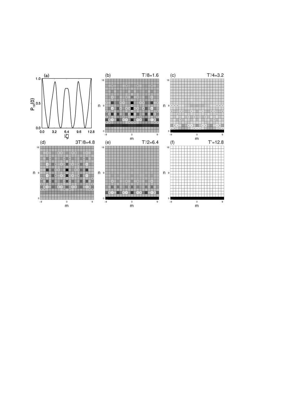
Fig. 1.10: Generalized squeezed vacuum: (a) Vacuum-state probability, $P_{18}(0)=|b_{0}^{(18)}|^{2}$, for $|\zeta\rangle_{(18)}$ as a function of the squeeze parameter amplitude $|\zeta|$; (b–f) Wigner function for $|\zeta\rangle_{(18)}$ with $\zeta$ given by fractions of the quasiperiod $T^{\prime}=T^{\prime}_{18}=12.8$.

1. Generalized Squeezed Vacuum

By analogy with the conventional squeezed vacuum [68], we define the generalized squeezed vacuum in the ($s+1$)-dimensional Hilbert space by [34]

$$|\zeta{\rangle\!_{(s)}}=\hat{S}_{s}(\zeta)\,|0\rangle$$ (1.80)

as the result of action of the generalized FD squeeze operator

$$\hat{S}_{s}(\zeta)=\exp\left\{{\textstyle\frac{1}{2}\,}(\zeta\hat{a}_{s}^{\dagger 2}-\zeta^{*}\hat{a}_{s}^{2})\right\}$$ (1.81)

on vacuum. Here, $\zeta=|\zeta|\exp({\mathrm{i}}\varphi)$ is the complex squeeze parameter; $\hat{a}_{s}$ and $\hat{a}_{s}^{\dagger}$ are, respectively, the FD annihilation and creation operators defined by Eq. (1.8). The method for finding explicit number-state representation of the generalized CS, presented in Appendix, can also be applied here. We find the following explicit Fock expansion of the generalized squeezed vacuum

$$|\zeta{\rangle\!_{(s)}}=\sum\limits_{n=0}^{\sigma}b_{2n}^{(s)}{\mathrm{e}}^{{\mathrm{i}}n\varphi}|2n\rangle$$ (1.82)

with the superposition coefficients given by

$$b_{2n}^{(s)}=(-{\mathrm{i}})^{n}\frac{(2\sigma)!}{\sqrt{(2n)!}}\sum\limits_{k=0}^{\sigma}\exp\left({\textstyle\frac{{\mathrm{i}}}{2}\,}|\zeta|x_{k}\right)\frac{G_{n}(x_{k})}{G_{\sigma}(x_{k})G_{\sigma+1}^{{}^{\prime}}(x_{k})}$$ (1.83)

where $\sigma=[\![s/2]\!]$ and $G_{n}(x)$ are the Meixner–Sheffer orthogonal polynomials defined by the recurrence relation [69]

$$G_{n+1}=xG_{n}-2n(2n-1)G_{n-1}\quad\quad$$ (1.84)

for $n=2,3,\dots$, together with $G_{0}(x)=1$ and $G_{1}(x)=x$. In Eq. (1.83), $x_{k}\equiv x_{k}^{(\sigma+1)}$ is the $k$th root ($k=0,\dots,\sigma$) of the polynomial $G_{\sigma+1}(x)$ and $G_{\sigma+1}^{\prime}({x_{k}})$ denotes the $x$-derivative at ${x=x_{k}}$. Since Eq. (1.83) is of a rather complicated form, we present a few examples of the FD squeezed vacuum for small dimensions. For $s$=2 and 3, we find

$$|\zeta{\rangle\!_{(2)}}=|\zeta{\rangle\!_{(3)}}=\cos\beta|0\rangle+{\mathrm{e}}^{{\mathrm{i}}\varphi}\sin\beta|2\rangle$$ (1.85)

where $\beta=\frac{1}{2}|\zeta x_{0}^{(2)}|=\frac{1}{\sqrt{2}}|\zeta|$. For $s=4,5$, we have

$$|\zeta\rangle\!_{(4)}=|\zeta\rangle\!_{(5)}={\textstyle\frac{1}{7}\,}(6+\cos\beta)|0\rangle+\;{\mathrm{e}}^{{\mathrm{i}}\varphi}{\textstyle\frac{1}{\sqrt{7}}\,}\sin\beta|2\rangle+\;{\mathrm{e}}^{2{\mathrm{i}}\varphi}{\textstyle\frac{2}{7}\,}\sqrt{6}\sin^{2}({\textstyle\frac{1}{2}\,}\beta)|4\rangle$$ (1.86)

where $\beta=\frac{1}{2}|\zeta x_{0}^{(3)}|=\sqrt{\frac{7}{2}}|\zeta|$. The generalized squeezed vacuum, given by (1.82), has more complicated form in Fock basis than that for the generalized CS, described by (1.22). In particular, the solution (1.83) contains rather complicated Meixner–Sheffer polynomials instead of the well-known Hermite polynomials, which occur in the expansions for the generalized CS.

Here, we discuss only a few basic properties of generalized squeezed vacuum, given by (1.80). By definition, it is properly normalized for arbitrary dimension of the Hilbert space. There are several ways to prove that the generalized squeezed vacuum goes over into the conventional squeezed vacuum ($|\zeta\rangle$) in the limit of $s\rightarrow\infty$. By definition (1.80), one can conclude that the property $\lim_{s\rightarrow\infty}|\zeta{\rangle\!_{(s)}}=|\zeta{\rangle\!_{(\infty)}}=|\zeta\rangle$ holds, since the FD annihilation and creation operators go over into the conventional ones: $\lim_{s\rightarrow\infty}\hat{a}_{s}=\hat{a}$ and $\lim_{s\rightarrow\infty}\hat{a}_{s}^{\dagger}=\hat{a}^{\dagger}$. One can also show, at least numerically, that the superposition coefficients (1.83) approach the coefficients $b_{n}$ for the conventional squeezed vacuum: $\lim_{s\rightarrow\infty}b^{(s)}_{n}=b_{n}$ for $n=0,\dots,s$. We apply another method based on the calculation of the scalar product $\langle\zeta|\zeta{\rangle\!_{(s)}}$. We show the analytical results for $|\zeta|\leq 1$ only. We have found the scalar product between conventional and generalized squeezed vacuums in the form (for even $s$)

$$\langle\zeta|\zeta{\rangle\!_{(s)}}=\langle\zeta|\zeta\rangle\!_{(s+1)}=1+\sum_{k=1}^{\infty}(-1)^{k}c_{k}^{(s)}|\zeta|^{s+2k}\leq 1$$ (1.87)

where the coefficients $c_{k}^{(s)}$ are positive and less than one for any $k$ and $s$. We find that the explicit expansion up to $|\zeta|^{s+2}$ can be given in terms of the binomial coefficient as follows

$$\langle\zeta|\zeta{\rangle\!_{(s)}}=\langle\zeta|\zeta{\rangle\!_{(s+1)}}=1-\left({{s+1}}\atop{{\frac{1}{2}s+1}}\right)\left(\frac{|\zeta|}{2}\right)^{s+2}+{\mathcal{}O}(|\zeta|^{s+4})$$ (1.88)

In particular, for $s=2,\dots,7$, we have

$$\langle\zeta|\zeta{\rangle\!_{(2)}}=\langle\zeta|\zeta{\rangle\!_{(3)}} = 1-\frac{3}{16}|\zeta|^{4}+\frac{1}{8}|\zeta|^{6}-{\mathcal{}O}(|\zeta|^{8})$$

$$\langle\zeta|\zeta{\rangle\!_{(4)}}=\langle\zeta|\zeta{\rangle\!_{(5)}} = 1-\frac{5}{32}|\zeta|^{6}+\frac{185}{1024}|\zeta|^{8}-{\mathcal{}O}(|\zeta|^{10})$$

$$\langle\zeta|\zeta{\rangle\!_{(6)}}=\langle\zeta|\zeta{\rangle\!_{(7)}} = 1-\frac{35}{256}|\zeta|^{8}+\frac{7}{30}|\zeta|^{10}-{\mathcal{}O}(|\zeta|^{12})$$ (1.89)

It is clearly seen that, for a given $\zeta$ , the scalar products become closer to unity with increasing space dimension. We conclude that the generalized state (1.80) approaches the conventional squeezed vacuum in the dimension limit.

2. Truncated Squeezed Vacuum

One can propose another definition of a FD squeezed vacuum, such as by truncation of the Fock expansion of the conventional squeezed vacuum at the state $|s\rangle$. Thus, we define the truncated squeezed vacuum as follows [34]

$$|{\overline{\zeta}\,}{\rangle\!_{(s)}}=\sum\limits_{n=0}^{\sigma+1}{b}_{2n}^{(s)}{\mathrm{e}}^{{\mathrm{i}}n\varphi}|2n\rangle$$ (1.90)

with the superposition coefficients

$${b}_{2n}^{(s)}={\mathcal{}N}_{s}\frac{\sqrt{(2n)!}}{n!}{t}^{n}$$ (1.91)

normalized by

$${\mathcal{}N}_{s}^{-2}=\cosh|{\overline{\zeta}\,}|-2t^{2\sigma+2}{2\sigma+1\choose\sigma}\,{\mathrm{}2F_{1}}\!(1,\left\{{\textstyle\frac{3}{2}\,}+\sigma,2+\sigma\right\},4t^{2})$$ (1.92)

where $\sigma=[\![s/2]\!]$; $t=\frac{1}{2}\tanh|{\overline{\zeta}\,}|$, and ${\mathrm{}2F_{1}}$ is the generalized hypergeometric function. We marked with a bar the complex squeeze parameter ${\overline{\zeta}\,}$ for the truncated states in order to distinguish it from the generalized squeezed vacuum defined by applying the FD squeeze operator. We give an example of the truncated squeezed vacuum. For $s=2,3$, Eq. (1.90) reduces to

$$|{\overline{\zeta}\,}{\rangle\!_{(2)}}=|{\overline{\zeta}\,}{\rangle\!_{(3)}}=\frac{|0\rangle+\sqrt{2}t|2\rangle}{\sqrt{1+2t^{2}}}$$ (1.93)

The state (1.90), by definition, goes over into the conventional squeezed vacuum in the limit of large dimension: $\lim_{s\rightarrow\infty}|{\overline{\zeta}\,}{\rangle\!_{(s)}}=|{\overline{\zeta}\,}\rangle\equiv|\zeta\rangle$. We can explicitly show this by expanding the scalar products between them in power series with respect to $|\zeta|^{2}=|{\overline{\zeta}\,}|^{2}\ll s$. We find (for even $s$)

$${{}_{(\infty)}\!\langle}\zeta|{\overline{\zeta}\,}{\rangle\!_{(s)}}={{}_{(\infty)}\!\langle}\zeta|{\overline{\zeta}\,}{\rangle\!_{(s+1)}}$$ (1.94)

under assumption $\varphi=\overline{\varphi}$. In particular, we have

$${{}_{(\infty)}\!\langle}\zeta|{\overline{\zeta}\,}{\rangle\!_{(2)}}={{}_{(\infty)}\!\langle}\zeta|{\overline{\zeta}\,}{\rangle\!_{(3)}} = 1-\frac{3}{16}|\zeta|^{4}+\frac{3}{16}|\zeta|^{6}-{\mathcal{}O}(|\zeta|^{8})$$

$$\langle\zeta|{\overline{\zeta}\,}{\rangle\!_{(4)}}=\langle\zeta|{\overline{\zeta}\,}{\rangle\!_{(5)}} = 1-\frac{5}{32}|\zeta|^{6}+\frac{65}{256}|\zeta|^{8}-{\mathcal{}O}(|\zeta|^{10})$$

$$\langle\zeta|{\overline{\zeta}\,}{\rangle\!_{(6)}}=\langle\zeta|{\overline{\zeta}\,}{\rangle\!_{(7)}} = 1-\frac{35}{256}|\zeta|^{8}+\frac{119}{384}|\zeta|^{10}-{\mathcal{}O}(|\zeta|^{10})$$ (1.95)

We can also explicitly compare $|{\overline{\zeta}\,},2n_{0}{\rangle\!_{(s)}}$ with $|\zeta,2n_{0}{\rangle\!_{(s)}}$ with the help of their scalar products. In particular, by putting $\varphi=\overline{\varphi}$, we have

$${{}_{(2)}\!\langle}\zeta|{\overline{\zeta}\,}{\rangle\!_{(2)}}={{}_{(2)}\!\langle}\zeta|{\overline{\zeta}\,}{\rangle\!_{(3)}} = 1-\frac{1}{16}|\zeta|^{6}+\frac{7}{80}|\zeta|^{8}-{\mathcal{}O}(|\zeta|^{10})$$

$${{}_{(4)}\!\langle}\zeta|{\overline{\zeta}\,}{\rangle\!_{(4)}}={{}_{(5)}\!\langle}\zeta|{\overline{\zeta}\,}{\rangle\!_{(5)}} = 1-\frac{75}{2^{10}}|\zeta|^{8}+\frac{131}{2^{10}}|\zeta|^{10}-{\mathcal{}O}(|\zeta|^{12})$$

$${{}_{(6)}\!\langle}\zeta|{\overline{\zeta}\,}{\rangle\!_{(6)}}={{}_{(7)}\!\langle}\zeta|{\overline{\zeta}\,}{\rangle\!_{(7)}} = 1-\frac{49}{640}|\zeta|^{10}+\frac{189}{2^{10}}|\zeta|^{12}-{\mathcal{}O}(|\zeta|^{14})$$ (1.96)

By comparing Eq. (1) with Eqs. (1.89) and (1), we can conclude that the differences between the generalized and truncated squeezed vacuums are smaller than those between them and the conventional squeezed vacuum. All these states coincide in the high-dimension limit. In Fig. 1.10b–f, we have presented the Wigner representation of the generalized squeezed vacuum for those values of the squeeze parameter $|\zeta|$, which correspond to maximum and minimum values of the vacuum-state probability given by $P_{s}(0)=|b^{(s)}_{0}|^{2}$ (see Fig. 1.10a). We find that the generalized squeezed vacuum is quasiperiodic in $|\zeta|$. Although, its quasiperiod $T^{\prime}_{s}$ differs from $T_{s}$ for the generalized CS, phase CS, displaced number states or Schrödinger cats, as given by Eqs. (1.34) and (1.35). The truncated squeezed vacuum is aperiodic in $|{\overline{\zeta}\,}|$, similarly to other truncated quantum-optical states discussed in Sections IV and V.

VI.  CONCLUSION

We have compared two approaches to define finite-dimensional (FD) analogs of the conventional quantum-optical states of infinite-dimensional Hilbert space. We have contrasted (1) the generalized coherent states (CS), defined by the action of the generalized FD displacement operator on vacuum, with (2) the truncated CS, defined by the normalized truncated Fock expansion of the conventional Glauber CS. We have shown both analytically and graphically that these CS constructed in FD Hilbert spaces exhibit essentially different behaviors; the generalized CS are periodic (for $s$=1,2) or quasiperiodic (for higher $s<\infty$) functions of the displacement parameter, whereas the truncated CS are aperiodic for any $s$ (even for $s$=1). Both the generalized and truncated CS go over into the conventional CS in the dimension limit. Nevertheless, the truncated CS approach the conventional Glauber CS faster than the generalized CS do. Besides, as the special case, we have compared in detail the two-dimensional CS. We have analyzed other finite-dimensional quantum-optical states. In particular, we have discussed: (1) FD phase coherent states, (2) FD displaced number states; (3) FD Schrödinger cats (including even and odd CS); and (4) FD squeezed vacuums. We have confronted two essentially different ways of defining states in FD Hilbert spaces. We have constructed explicitly all of these states generated by various finite-dimensional displacement or squeeze operators using the method developed in Ref. [18] for the generalized CS. We have also presented graphical representations of the discrete number-phase Wigner function, which enabled us a very intuitive understanding of the properties of the generalized and truncated quantum-optical states.

APPENDIX

Here, after Ref. [18], we present a method for finding the coefficients $b^{(s)}_{n}$ of Fock representation of the generalized CS, given by Eq. (1.22).

The Baker-Hausdorf formula cannot be used to solve this problem because the commutator of the annihilation $\hat{a}_{s}$ and creation $\hat{a}_{s}^{\dagger}$ operators is not a $c$-number. A numerical procedure, leading to the coefficients $b^{(s)}_{n}$, was proposed by Bužek et al. [16]. In order to solve this problem analytically [18], it is of advantage to express the conventional coherent state, $|\alpha\rangle$, in the Fock representation in a different manner

$$|\alpha\rangle = \sum_{n=0}^{\infty}\frac{(\alpha a^{\dagger}-\alpha^{*}a)^{n}}{n!}|0\rangle$$ (A.1)

$$= \sum_{n=0}^{\infty}\sum_{k=0}^{[\![n/2]\!]}\frac{\sqrt{(n-2k)!}}{n!}\ d_{n,n-2k}(-\alpha^{*})^{k}\alpha^{n-k}|n-2k\rangle$$

where

$$d_{n,k} = \left({n\atop k}\right)(n-k-1)!!$$ (A.2)

and $[\![x]\!]$ is the integer part of $x$. Thus, Eq. (A.1) for the generalized CS can be rewritten as

$$|\alpha{\rangle\!_{(s)}}=\sum_{k=0}^{s}\left[\sum_{n=k}^{\infty}\frac{\sqrt{k!}}{n!}\ d^{(s)}_{nk}(-\alpha^{*})^{(n-k)/2}\alpha^{(n+k)/2}\right]\,|k\rangle\equiv\sum_{k=0}^{s}c^{(s)}_{k}|k\rangle$$ (A.3)

The problem reduces to derivation of the coefficients $d^{(s)}_{n,k}$ satisfying the condition in the dimension limit

$$\lim\limits_{s\rightarrow\infty}d_{nk}^{(s)}\;=\;d_{n,k}^{(\infty)} \equiv d_{nk}\>=\>\left(n\atop k\right)\,(n-k-1)!!$$ (A.4)

We obtain the following simple recurrence formula

$$d_{nk}^{(s)} = \theta_{k}d_{n-1,k-1}^{(s)}+(k+1)\theta_{k+1}d_{n-1,k+1}^{(s)}$$ (A.5)

with the conditions $d_{00}^{(s)}=1$ and $d_{n,n+k}^{(s)}=0$ for $s,k>0$. In Eq. (A.5), $\theta_{n}$ is the Heaviside function defined to be

$$\theta_{n}\equiv\theta(s-n)=\left\{{1\quad\mbox{for}\quad s\geq n}\atop{0\quad\mbox{for}\quad s<n}\right.$$ (A.6)

The solution of the recurrence formula (A.5) is

$$d_{nk}^{(s)} = \frac{s!}{k!(s+1)}\sum_{l=0}^{s}\frac{{\mathrm{H}e}_{k}(x_{l})}{[{\mathrm{H}e}_{s}(x_{l})]^{2}}x_{l}^{n}$$ (A.7)

where $x_{l}\equiv x^{(s+1)}_{l}$ are the roots of the Hermite polynomial ${\mathrm{H}e}_{s+1}(x)$. A solution similar to ours (A.7) was found by Figurny et al. [32] in their analysis of the eigenvalues of the truncated quadrature operators. On performing summation in Eq. (A.3) with the coefficients $d_{nk}^{(s)}$, given by (A.7), one readily arrives at

$$C_{n}^{(s)}=\frac{s!}{s+1}\frac{1}{\sqrt{n!}}\sum_{k=0}^{s}\exp\left\{{\mathrm{i}}[n(\varphi-\pi/2)+x_{k}\,|\alpha|]\right\}\frac{{\mathrm{H}e}_{n}(x_{k})}{[{\mathrm{H}e}_{s}(x_{k})]^{2}}\equiv{\mathrm{e}}^{{\mathrm{i}}n\varphi}b_{n}^{(s)}$$ (A.8)

or, equivalently, Eq. (1.23). Our procedure provides the coefficients $b^{(s)}_{n}$ in a closed analytical form. This is the solution of the problem formulated by Bužek et al. [16].

ACKNOWLEDGMENTS

A. M. and W. L. thank J. Bajer, S. Dyrting, M. Koashi, T. Opatrný, Ş. K. Özdemir, J. Peřina, K. Pia̧tek, and R. Tanaś for their stimulating discussions. A. M. is indebted to Prof. Nobuyuki Imoto for his hospitality at SOKEN.

REFERENCES

Index

Characteristic function, 6

Coherent states; generalized, 9

Coherent states; truncated, 13

Coherent states; two-dimensional, 17

Displaced number states; generalized, 23

Displaced number states; truncated, 24

Displacement operator, 9

Even coherent states, 25

Finite-dimensional Hilbert space, 1, 3

Hermite polynomial, 10, 12, 21, 33

Meixner–Sheffer orthogonal polynomials, 29

Odd coherent states, 25

Pegg–Barnett phase distribution, 8

Pegg–Barnett phase formalism, 2

Phase coherent states; generalized, 20

Phase coherent states; truncated, 21

Phase displacement operator, 21

Phase operator, 4

Phase states, 4

Photon-number distribution, 8

Poincaré sphere, 18

Quantum scissors, 2

Schrödinger cats; generalized, 25

Schrödinger cats; truncated, 26

Squeeze operator, 28

Squeezed vacuum; generalized, 28

Squeezed vacuum; truncated, 30

Squeezing; degree, 19

Stokes parameters, 18

Wigner function; discrete, 3, 5

REFERENCES

- 1. H. Weyl, Theory of Groups and Quantum Mechanics, Dover, New York, 1931.
- 2. J. Schwinger, Proc. Natl. Acad. Sci. (USA) 46, 570 (1960); reprinted in Quantum Kinematics and Dynamics, Benjamin, New York, 1970, p. 63.
- 3. T. S. Santhanam and A. R. Tekumalla, Found. Phys. 6, 583 (1976); T. S. Santhanam, Phys. Lett. A 56, 345 (1976); T. S. Santhanam and K. B. Sinha, Aust. J. Phys. 31, 233 (1978); T. S. Santhanam, in B. Gruber and S. Millmann (Eds.), Symmetries in Science, Plenum, New York, 1980, p. 337.
- 4. J. M. Radcliffe, J. Phys. A 4, 313 (1971).
- 5. C. Arecchi, E. Courtens, R. Gilmore and H. Thomas, Phys. Rev. A 6, 2211 (1972).
- 6. R. J. Glauber and F. Haake, Phys. Rev. A 13, 357 (1976).
- 7. E. Schrödinger, Naturwissenschaften 14, 664 (1926).
- 8. R. J. Glauber, Phys. Rev. 130, 2529 (1963); ibid. 131, 2766 (1963).
- 9. E. C. G. Sudarshan, Phys. Rev. Lett. 10, 277 (1963).
- 10. A. M. Perelomov, Commun. Math. Phys. 26, 222 (1972); Usp. Fiz. Nauk 123, 23 (1977) [Sov. Phys. Usp. 20, 703 (1977)]; Generalized Coherent States and their Applications, Springer, Berlin, 1986.
- 11. R. Gilmore, Ann. Phys. (N.Y.) 74, 391 (1972); Rev. Mex. Fis. 23, 142 (1974); J. Math. Phys. 15, 2090 (1974).
- 12. W. M. Zhang, D. H. Feng, and R. Gilmore, Rev. Mod. Phys. 62, 867 (1990).
- 13. I. A. Malkin and V. I. Man’ko, Dynamical Symmetries and Coherent States of Quantum Systems, Nauka, Moscow, 1979.
- 14. J. R. Klauder and B. S. Skagerstam (Eds.), Coherent States: Applications in Physics and Mathematical Physics, World Scientific, Singapore, 1985.
- 15. D. H. Feng and J. Klauder (Eds.), Coherent States: Past, Present and Future, World Scientific, Singapore, 1994.
- 16. V. Bužek, A. D. Wilson-Gordon, P. L. Knight, and W. K. Lai, Phys. Rev. A 45, 8079 (1992).
- 17. L. M. Kuang, F. B. Wang, and Y. G. Zhou, Phys. Lett. A 183, 1 (1993); J. Mod. Opt. 41, 1307 (1994).
- 18. A. Miranowicz, K. Pia̧tek, and R. Tanaś, Phys. Rev. A 50, 3423 (1994).
- 19. A. K. Pati and S. V. Lawande, Phys. Rev. A 51, 5012 (1995).
- 20. T. Opatrný, A. Miranowicz, and J. Bajer, J. Mod. Opt. 43, 417 (1996).
- 21. A. Miranowicz, T. Opatrný, and J. Bajer, in T. Hakioǧlu and A. S. Shumovsky (Eds.), Quantum Optics and the Spectroscopy of Solids: Concepts and Advances, Vol. 83, Fundamental Theories of Physics, Kluwer, Dordrecht, 1997, p. 225.
- 22. B. Roy and R. Roychoudhury, Int. J. Theor. Phys. 36, 1525 (1997).
- 23. B. Roy, Modern Phys. Lett. B 11, 963 (1997).
- 24. B. Roy and P. Roy, J. Phys. A 31, 1307 (1998).
- 25. J. Y. Zhu and L. M. Kuang, Phys. Let. A 193, 227 (1994); Chinese Phys. Lett. A 11, 424 (1994).
- 26. D. T. Pegg, and S. M. Barnett, Europhys. Lett. 6, 483 (1988); Phys. Rev. A 41, 3427 (1989); S. M. Barnett and D. T. Pegg, J. Mod. Opt. 36, 7 (1989).
- 27. L. M. Kuang and X. Chen, Phys. Rev. A 50, 4228 (1994); Phys. Lett. A 186, 8 (1994).
- 28. G. Gangopadhyay, J. Mod. Opt. 41, 525 (1994).
- 29. A. Miranowicz, K. Pia̧tek, T. Opatrný, and R. Tanaś, Acta Phys. Slov. 45, 391 (1995).
- 30. P. Roy and B. Roy, Quantum and Semiclas. Optics 9, L37 (1997).
- 31. K. Wódkiewicz, P. L. Knight, S. J. Buckle, and S. M. Barnett, Phys. Rev. A 35, 2567 (1987).
- 32. P. Figurny, A. Orłowski, and K. Wódkiewicz, Phys. Rev A 47, 5151 (1993).
- 33. D. J. Wineland, J. J. Bollinger, W. M. Itano, and D. J. Heinzen, Phys. Rev. A 50, 67 (1994).
- 34. A. Miranowicz, W. Leoński, and R. Tanaś, in D. Han et al. (Eds.), NASA Conference Publication 206855, Greenbelt, MD, 1998, p. 91.
- 35. L. M. Kuang and J. Y. Zhu, J. Phys. A 29, 895 (1996).
- 36. Special issue on quantum state preparation and measurement, J. Mod. Opt. 44 (11/12) (1997).
- 37. U. Leonhardt, Phys. Rev. Lett. 74, 4101 (1995); ibid. 76, 4293 (1996); Phys. Rev. A 53, 2998 (1996).
- 38. V. I. Man’ko, O. V. Man’ko, JETP 85, 430 (1997); V. A. Andreev, V. I. Man’ko, JETP 87, 239 (1998); V. I. Man’ko, S. S. Safonov, Phys. Atom. Nuclei 61, 585 (1998).
- 39. V. Bužek, G. Drobný, G. Adam, R. Derka, P. L. Knight, J. Mod. Opt. 44, 2607 (1997); V. Bužek, R. Derka, G. Adam, P. L. Knight, Ann. Phys. (San Diego) 266, 454 (1998).
- 40. R. Walser, J. I. Cirac, P. Zoller, Phys. Rev. Lett. 77, 2658 (1996).
- 41. J. -P. Amiet and S. Weigert, J. Phys. A 31 L543 (1998); ibid. 32 L269 (1999); J. Opt. B 1 L5 (1999).
- 42. D. -G. Welsch, W. Vogel, and T. Opatrný, in E. Wolf (Ed.), Progress in Optics, Vol. 39, North-Holland, Amsterdam, 1999, p. 63.
- 43. R. Tanaś, A. Miranowicz, and T. Gantsog, in E. Wolf (Ed.), Progress in Optics, Vol. 35, North-Holland, Amsterdam, 1996, p. 355.
- 44. D. T. Pegg, L. S. Phillips, and S. M. Barnett, Phys. Rev. Lett. 81, 1604 (1998); S. M. Barnett and D. Pegg, Phys. Rev. A 60, 4965 (1999).
- 45. M. Koniorczyk, Z. Kurucz, A. Gábris, and J. Janszky, Phys. Rev. A 62, 013802 (2000).
- 46. M. G. A. Paris, Phys.Rev. A 62, 033813 (2000).
- 47. A. Miranowicz, Ş. K. Özdemir, N. Imoto, and M. Koashi, Mtg. Abstr. Phys. Soc. Jpn. 62, 108 (2000).
- 48. W. Leoński and R. Tanaś, Phys. Rev. A 49, R20 (1994); W. Leoński, Phys. Rev. A 54, 3369 (1996); W. Leoński, S. Dyrting, and R. Tanaś, J. Mod. Opt. 44, 2105 (1997).
- 49. W. Leoński, Phys. Rev. A 55, 3874 (1997).
- 50. A. Miranowicz, W. Leoński, S. Dyrting, and R. Tanaś, Acta Phys. Slov. 46, 451 (1996).
- 51. W. Leoński and A. Miranowicz, “Quantum-optical states in finite-dimensional Hilbert space. II. State generation”, Chapter 4, this volume.
- 52. E. P. Wigner, Phys. Rev. 40, 749 (1932); for a review, see M. Hillery, R. F. O’Connell, M. O. Scully, and E. P. Wigner, Phys. Rep. 106, 121 (1984); V. I. Tatarskii, Sov. Phys. Usp. 26, 311 (1983).
- 53. R. L. Stratonovich, Sov. Phys. JETP 4, 891 (1957); L. Cohen and M. O. Scully, Found. Phys. 16, 295 (1986).
- 54. R. F. O’Connell, and E. P. Wigner, Phys. Rev. A 30, 2613 (1984).
- 55. W. K. Wootters, Ann. Phys. 176, 1 (1987).
- 56. O. Cohendet, P. Combe, M. Sirugue, and M. Sirugue-Collin, J. Phys. A 21, 2875 (1988).
- 57. J. A. Vaccaro and D. T. Pegg, Phys. Rev. A 41, 5156 (1990).
- 58. T. Opatrný, V. Bužek, J. Bajer, and G. Drobný, Phys. Rev. A 52, 2419 (1995).
- 59. T. Opatrný, D. -G. Welsch, and V. Bužek, Phys. Rev. A 53, 3822 (1996).
- 60. T. Hakioǧlu, J. Phys. A 31, 6975 (1998).
- 61. A. Lukš and V. Peřinová, Phys. Scr. T 48, 94 (1993).
- 62. A. Luis and J. Peřina, J. Phys. A 31, 1423 (1998).
- 63. J. Peřina, Z. Hradil, and B. Jurčo, Quantum Optics and Fundamentals of Physics, Vol. 63, Fundamental Theories in Physics, Kluwer Academic, Dordrecht, 1994.
- 64. W. Leoński and A. Miranowicz, Acta Phys. Slov. 46, 433 (1996); W. Leoński, A. Miranowicz, and R. Tanaś, Laser Physics 7, 126 (1997).
- 65. F. A. M. de Oliveira, M. S. Kim, P. L. Knight, and V. Bužek, Phys. Rev. A 41, 2645 (1990).
- 66. V. Bužek, and P. L. Knight, in E. Wolf (Ed.), Progress in Optics, Vol. 34, North-Holland, Amsterdam, 1995, p. 1.
- 67. A. Miranowicz, R. Tanaś, and S. Kielich, Quantum Opt. 2, 253 (1990).
- 68. R. Loudon and P. L. Knight, J. Mod. Opt. 34, 709 (1987); K. Zaheer and M. S. Zubairy, in D. Bates and B. Bederson (Eds.), Advances in Atomic, Molecular and Optical Physics, Vol. 28, Academic Press, New York, 1990, p. 143.
- 69. J. Meixner, J. London Math. Soc. 9, 6 (1934); I. M. Sheffer, Duke Math. J. 5, 590 (1939).
Index