Geometric phases of mesoscopic spin in Bose-Einstein condensates

Abstract

We propose a possible scheme for generating spin-$J$ geometric phases using a coupled two-mode Bose-Einstein condensate (BEC). First we show how to observe the standard Berry phase using Raman coupling between two hyperfine states of the BEC. We find that the presence of intrinsic interatomic collisions creates degeneracy in energy that allows implementation of the non-Abelian geometric phases as well. The evolutions produced can be used to produce interference between different atomic species with high numbers of atoms or to fine control the difference in atoms between the two species. Finally, we show that errors in the standard Berry phase due to elastic collisions may be corrected by controlling inelastic collisions between atoms.

I INTRODUCTION

Geometrical phases in quantum theory have attracted considerable interest since Berry [1] showed that the state of a system undergoing an adiabatic and cyclic evolution acquires this purely geometric feature in addition to the usual dynamical phase. The term ”geometric” comes from the fact that the phase factor acquired by the state depends only on the path followed by the state but not on the rate at which it is traversed. If the system is nondegenerate, the geometric phase is simply a complex number called the Abelian phase, but in general it is a unitary matrix inducing transitions between degenerate states, which is called the non-Abelian phase or holonomy [2]. Geometric phases have been proposed [3] and tested [4] in a variety of settings. Generalizations of Berry’s phase analysis to nonadiabatic, noncyclic, and nonunitary evolutions have also been achieved [5]. Sjöqvist et. al. proposed an operationally well defined generalization of the geometric phase for mixed states [6] and more recently, a fully quantized version of the phase has been given that considers vacuum induced effects [7]. Holonomies and Berry phases have relevance in implementing quantum computation [8], where a universal set of quantum gates can be performed in a fault-tolerant way by a succession of geometrical unitaries [9]. Moreover, geometric evolution of states may also have importance in manipulating quantum systems such as Bose-Einstein condensates (BECs). For example, a certain type of geometric phase have been used to create vortices in BECs [10]. In this paper, we propose a method of testing both Abelian and non-Abelian geometric phases for a general spin-$J$ system modeled by two coupled Bose-Einstein condensates. This is interesting, because it allows us to test geometric phases for spin values as mesoscopic as $J\sim 10^{4}$, a feat not accomplished yet in any other system.

Trapped atomic BECs, first achieved some seven years ago, provide us with the ability to make mesoscopic quantum objects containing of the order 10⁶ atoms in the same quantum state. Although a mesoscopic system may, in principle, be constructed using photons as well, a crucial distinction is that atoms may be stored for longer times. A longer storage time (of the order of an hour for magnetic traps [11]) implies a longer decoherence time scale of quantum states, thereby aiding the implementation of adiabatic evolution (required for the Berry phase). Geometrical phases are generated by adiabatically varying the Hamiltonian of a system in a cyclic fashion. This can be done in BECs since the states of ultracold atomic samples can be manipulated by electromagnetic fields.

The Hamiltonian describing a fixed number of atoms in two different internal levels trapped by a magnetic potential can be approximated, for systems composed of a few thousand atoms, by a two-mode Hamiltonian [12, 13]. The Schwinger oscillator model allows to conveniently express the two-mode problem in terms of angular momentum operators. In this way the Abelian and non-Abelian phases generated are associated with spin-$J$ states, where the spin is related to the total number of atoms in the condensate. We use two-photon excitations, which generate a coherent superposition in the two-mode BEC, to demonstrate the Berry phase when the collisions between atoms are neglected. We then extend this idea further to consider the possibility of measuring holonomies including the nonlinear term due to collisional interaction between particles for which the Hamiltonian is degenerate. To produce Abelian and non-Abelian transformations when the non-linear term in the Hamiltonian is considered, in addition to the two-photon excitations, inelastic collisions must be manipulated. Together the two-photon excitations and the inelastic collisions correspond to a two-mode displacement of the eigenstates of the system and this may have potential applications in manipulating BECs. We shall show that, if collisions between atoms are seen as errors in the Berry phase generated by the linear Hamiltonian, these errors can be corrected by introducing inelastic collisions.

The paper is organized as follows. In Sec. II we describe, using angular momentum operators, the physical system we consider for generating geometric phases: the two-mode BEC. Section III is devoted to explain how Berry phases and holonomies arise, presenting the main mathematical formalism used through the paper. In section IV we discuss how to generate Berry phase in the BEC described in section II and we propose a scheme for detecting this phase. In Sec. V we move to consider the holonomies related to the two-mode BEC. Section VI contains final remarks concerning the generation of the Berry phase when collisions between the atoms in the condensates cannot be neglected, and finally the paper concludes in Sec. VII.

II THE TWO-MODE BOSE-EINSTEIN CONDENSATE

A physical realization of our system is two condensates in different hyperfine levels $|A\rangle$ and $|B\rangle$, such as those already produced in experiments by Myatt et. al [14] and Stenger et. al [15]. In the Rb system of Ref.[14], an external laser is applied to induce a Josephson-like coupling and the detuning of the laser is adiabatically changed to produce various transitions. Alternatively, for the Na spinor system of Ref. [15], state-dependent magnetic field gradient may be applied to induce Josephson tunneling. The Hamiltonian for the system can be written under the two-mode approximation, taking the annihilation operators to be $a$ and $b$ for the two distinct hyperfine states:

$$H = H_{a}+H_{b}+H_{int}+H_{las},$$ (1)

$$H_{a} = \omega_{a}a^{\dagger}a+\frac{U_{a}}{2}a^{\dagger}a^{\dagger}aa,$$ (2)

$$H_{b} = \omega_{b}b^{\dagger}b+\frac{U_{b}}{2}b^{\dagger}b^{\dagger}bb,$$ (3)

$$H_{int} = \frac{U_{ab}}{2}a^{\dagger}ab^{\dagger}b,$$ (4)

$$H_{las} = -\lambda(a^{\dagger}be^{-i\Delta t}+b^{\dagger}ae^{i\Delta t}),$$ (5)

where $H_{a}$ and $H_{b}$ describe the two condensates undergoing self-interactions and $H_{int}$ and $H_{las}$ describe the condensates interacting with one another via collisional and laser-induced interactions, respectively. $\Delta$ is the detuning of the laser from the $|A\rangle\rightarrow|B\rangle$ transition. We note in particular that $H_{las}$ describes Josephson-like coupling which interchanges internal atomic states in a coherent manner.

As discussed above, the Hamiltonian can be written in a more suitable way by employing the Schwinger angular momentum [$SU(2)$] operators defined as $J_{x}=\frac{1}{2}(a^{\dagger}b+ab^{\dagger}),J_{y}=(1/2i)(a^{\dagger}b-ab^{\dagger}),andJ_{z}=\frac{1}{2}(a^{\dagger}a-b^{\dagger}b)$. The Casimir invariant $J^{2}=J_{x}^{2}+J_{y}^{2}+J_{z}^{2}$ has eigenvalues $j(j+1)$ and $j$ represents the total number $2N=2(N_{A}+N_{B})$ of the two different species of atoms ($N$ could be $10^{4}$ for the type of condensates we consider). In terms of Schwinger operators, the Hamiltonian takes the simple form

$$H=\alpha J_{z}+\beta J_{z}^{2}+\gamma[\cos(\phi)J_{x}+\sin(\phi)J_{y}]$$ (6)

where $\alpha=\omega_{a}-\omega_{b}+(2J-1)(U_{a}-U_{b})/2$, $\beta=(U_{a}+U_{b}-U_{ab})/2$, and $\phi=\Delta t$. The eigenvalues $m$ of the operator $J_{z}$ represents the difference $2(N_{A}-N_{B})$ in the number of atoms in different hyperfine levels, while $J_{x}$ (and $J_{y}$) takes on the meaning of the relative phase between the two species. It is noted here that $s$-wave scattering lengths may be tuned using Feshbach resonances by the application of an external magnetic field[16]. The factors $U_{a}$, $U_{b}$, $U_{ab}$, and consequently $\alpha$ and $\beta$ are therefore adjustable parameters giving us important additional degrees of freedom. The above Hamiltonian [Eq.(6)] is sufficient to generate the Abelian Berry phase if the collision term ($\beta J_{z}^{2}$) is negligible. We shall describe later how terms such as $J_{x}J_{y}$ and $J_{x}^{2}$ (required for the non-Abelian geometric phase) can be added to the above Hamiltonian by inducing inelastic collisions.

III Geometric Evolutions

We will now describe briefly how geometric phases arise. Holonomies are unitary transformations of geometric origin generated by varying a set of external parameters $\sigma=\{\sigma_{\mu}\}_{\mu=0}^{k}$ featuring in the Hamiltonian of a system, in a cyclic and adiabatic way. Their dimensionality $n$ equals the degree of degeneracy of the eigenspace. The Berry phase is the special case when the eigenspace is nondegenerate, and the unitary transformation is then one dimensional, i.e., a complex number. Consider that the adiabatic variation of the Hamiltonian is given by $H(\sigma)={\cal U}(\sigma)H_{0}{\cal U}^{\dagger}(\sigma)$ (where the parameters $\sigma$ vary on some control manifold $\mathcal{M}$) with the ${\cal U}(\sigma)$ transformation being such that the degeneracy structure of the initial Hamiltonian $H_{0}$ is preserved. For this purpose, the parameters must be varied slowly with respect to any time scale associated with the system dynamics. After $\sigma$ completes a loop $C$ in $\mathcal{M}$, an initially prepared state $|\Psi_{in}\rangle$ is mapped to $|\Psi_{out}\rangle=e^{-iET}\Gamma_{A}(C)|\Psi_{in}\rangle$ where $T$ is the overall time of the evolution, and $E$ is the energy of the degenerate space where $|\Psi_{in}\rangle$ and $|\Psi_{out}\rangle$ belong. $\Gamma_{A}(C)$ (termed the holonomy associated with non-Abelian connection forms) appears due to the nontrivial topology structure of the degenerate space and is given by

$$\Gamma_{A}(C)={\bf P}\exp{\int_{C}A}\,\,.$$ (7)

$\bf{P}$ is the path ordering symbol and the Wilczek-Zee connection $A$ [2] is defined as

$$A^{\mu}_{ij}:\equiv\langle i|{\cal U}^{\dagger}(\sigma)\frac{\partial}{\partial\sigma_{\mu}}{\cal U}(\sigma)|j\rangle$$ (8)

for $i,j=1,...,n$ parametrizing states belonging to the same degenerate eigenspace of $H_{0}$.

An alternative interpretation of the holonomy, which is needed here to calculate explicitly the integral in Eq. (7), is that the holonomy can be seen as the exponential of the flux of the field strength $F_{\sigma\tau}(\sigma,\tau)=-\partial_{\sigma}A_{\tau}+\partial_{\tau}A_{\sigma}+[A_{\sigma},A_{\tau}]$, through a surface parametrized by $\sigma$ and $\tau$. If we consider the surface to be a rectangular loop $C$ in the plane $(\sigma,\tau)$ with ordered sides $1$, $2$, $3$ and $4$ , and represent the path order exponential integrals of the connection for each side by $W_{i}$ for $i=1,...,4$, for $T^{-1}(\sigma,\tau)=W_{4}W_{3}$ we can state the non-Abelian Stokes theorem [19] as

$$\Gamma_{A}(C)=W_{4}W_{3}W_{2}W_{1}={\bf P}_{\tau}e^{\int_{\Sigma(C)}T^{-1}F_{\sigma\tau}Td\sigma d\tau}\,\,,$$ (9)

where ${\bf P}_{\tau}$ is the path ordering symbol with respect to the $\tau$ variable only, unlike the usual path ordering symbol P, which is with respect to both variables $\sigma$ and $\tau$. The evaluation of the holonomies here is performed by the application of (9).

IV SPIN J BERRY PHASE

To generate a Berry phase in the BEC, let us first ignore the terms in the Hamiltonian due to collisions. A BEC can be described by such a Hamiltonian when one may assume that the condensate is dilute enough that the collisional interactions between the atoms (both inter- and intraspecies) become insignificant compared to the coupling rate generated by the strong external field. In principle, one may also consider the case where through the Feshbach resonance $U_{a}+U_{b}=U_{ab}$ ($\beta=0$), or one can assume $U_{ab}=U_{a}=U_{b}$, and tune the scattering length of either one of the species so that either $U_{a}$ or $U_{b}$ is reduced down to zero energy[17]. Experimentally, one needs to ensure that losses due to three-body recombinations are minimized. In this case the nonlinear term in the Hamiltonian vanishes so that

$$H=\alpha J_{z}+\gamma[\cos(\phi)J_{x}+\sin(\phi)J_{y}].$$ (10)

This Hamiltonian corresponds to the motion of a spin $J$ particle in a magnetic field with amplitude $B=\sqrt{\alpha^{2}+\gamma^{2}}$, whose direction is slowly varying as $\phi$ changes. $\phi=\Delta t$ can be made to vary arbitrarily slowly (so that the adiabatic approximation holds true) by choosing arbitrarily small detuning $\Delta$. For a fixed $\gamma$, varying $\phi$ over a complete loop produces a nontrivial Berry phase. We now proceed to calculate this. The Hamiltonian can be written as

$$H(\phi,\theta)={\cal U}(\phi,\theta)H_{0}{\cal U}^{\dagger}(\phi,\theta)$$ (11)

where $H_{0}=\alpha_{0}J_{z}$ and ${\cal U}(\phi,\theta)=\exp(-i\phi J_{z})\exp(-i\theta J_{y})$ with $\alpha=\alpha_{0}\cos{\theta}$ and $\gamma=\alpha_{0}\sin{\theta}$. This unitary transformation on $H_{0}$ corresponds to a two-mode displacement with amplitude $\theta/2$ and phase $\phi$. The eigenvectors of $H_{0}$ are first rotated through an angle $\theta$ on the $xz$ plane and then rotated through an angle $\phi$ in the $xy$ plane (as shown in Fig.1) to obtain the eigenvectors of $H$. The eigenstates of $H_{0}$ are the usual angular momentum eigenstates with $J_{z}|j,m\rangle=m|j,m\rangle$. This implies that the eigenstates of our original Hamiltonian $H$ are $|\psi\rangle={\cal U}(\phi,\theta)|j,m\rangle$ and we can then calculate the Berry phase using expressions (7) and (8) for $i=j=m$. The connection components generated by the transformation ${\cal U}(\phi,\theta)$ for the eigenstates of $H_{0}$ are given by

$$A_{\phi} = \langle j,m|U^{\dagger}(\phi,\theta)\frac{\partial}{\partial\phi}U(\phi,\theta)|j,m\rangle$$ (12)

$$= -i\langle j,m|(\sin(\theta)J_{x}+\cos(\theta)J_{z})|j,m\rangle$$ (13)

$$= -im\cos{\theta}$$ (14)

and

$$A_{\theta} = \langle j,m|U^{\dagger}(\phi,\theta)\frac{\partial}{\partial\theta}U(\phi,\theta)|j,m\rangle$$ (15)

$$= -i\langle j,m|J_{y}|j,m\rangle=0.$$ (16)

The field strength is $F_{\phi,\theta}=im\sin\theta$ and we find that, if we vary $\theta$ from zero to a fixed value and $\phi$ from $0$ to $2\pi$, the state $|j,m\rangle$ acquires a phase

$$\phi^{m}_{Berry}=i\int_{0}^{2\pi}\int_{0}^{\theta}F_{\phi,\theta^{\prime}}d\theta^{\prime}d\phi=-2\pi m(1-\cos{\theta})\,\,,$$ (17)

which is $m$ times the solid angle subtended by the circuit at the origin in parameter space. During the evolution, the state also acquires a dynamical phase $\gamma^{m}_{dyn}=\int_{0}^{T}\langle j,m|H_{0}|j,m\rangle=m\alpha_{0}T$. This phase can be eliminated by choosing an adequate evolution time $T$ for which the dynamical phase is a multiple of $2\pi$. Note that the Berry phase does not depend on $T$ but only on the geometry of the loop $C$.

Now we shall discuss a scheme for detecting the Berry phase. We first prepare the system in the state $|j,j\rangle$, which, when represented in terms of the population of the two modes, is simply $|N\rangle\otimes|0\rangle$. We then switch on laser fields with detuning $\Delta=0$, and vary $\alpha$ and $\gamma$ slowly in such a way that $|j,j\rangle$ (following the Hamiltonian adiabatically) evolves to ${\cal U}(0,\pi/2)|j,j\rangle$. Now we implement an adiabatic loop of the Hamiltonian in the parameter space given by the transformation ${\cal U}^{\dagger}(0,\theta){\cal U}(2\pi,0){\cal U}(0,\theta)$, with $\cos{\theta}=1/2$. The middle transformation ${\cal U}(2\pi,0)$ is obtained by switching on the detuning $\Delta$ and letting the Raman transition on for a time such that $t=\frac{2\pi}{\Delta}$). If we choose the time of the loop of the Hamiltonian such that the dynamical phase is eliminated (i.e., a multiple of $2\pi$) for all states, then the evolution of the state during this loop will be purely due to geometric phases. Next, the transformation ${\cal U}^{\dagger}(0,\pi/2)$ is applied to the state. For our choice of $\theta$, the Berry phase will be such that the final state after all transformations will be orthogonal to $|j,j\rangle$ . The presence of a Berry phase can now be verified by measuring the population of the second mode, which will now always be nonzero. This method is a generalization of the usual Hadamard-Berry-Hadamard method used for the detection of the spin-$1/2$ Berry phase.

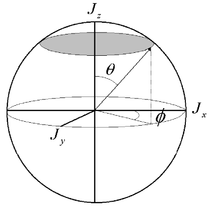
FIG. 1.: The spin-J Berry phase is obtained by rotating the eigenvectors of $H_{0}$ first through an angle $\theta$ in the $xz$ plane and then through an angle $\phi$ in the $xy$ plane. The phase is proportional to the area traversed by the vector.

V HOLONOMIC EVOLUTION IN THE TWO-MODE BEC

A geometric evolution in the condensate becomes a more complicated transformation when collisions are considered. The nonlinear term in the Hamiltonian allows for the possibility of degeneracy and, by slowly varying the Hamiltonian through the parameters, we can then generate holonomies. For performing a holonomic evolution the state of the system must be confined to a degenerate subspace at all times. A two-dimensional degenerate subspace can be created by making two of the eigenvalues of the Hamiltonian $H_{0}=\alpha_{0}J_{z}+\beta_{0}J_{z}^{2}$ equal. Choosing $\alpha_{0}/\beta_{0}=-(2m+1)$, the states $|j,m\rangle$ and $|j,m+1\rangle$ have the same energy. We shall transform the nonlinear Hamiltonian with the same unitary transformation that we used for the linear one, ${\cal U}(\phi,\theta)=\exp(-i\phi J_{z})\exp(-i\theta J_{y})$. This will result in a transformed Hamiltonian that includes inelastic collisions, but the states are transformed in the same manner as in the linear case. In particular, we obtain $U(\theta)H_{0}U^{\dagger}(\theta)=\alpha_{0}[\sin(\theta)J_{x}+\cos(\theta)J_{z})]+\beta_{0}[\sin^{2}(\theta)J_{x}^{2}+\cos^{2}(\theta)J_{z}^{2}+\sin(\theta)\cos(\theta)(2J_{x}J_{z}+1)]$. The term $J_{x}J_{z}$ includes inelastic collisions of the form $a^{\dagger}ba^{\dagger}a$, while $J_{x}^{2}$ includes terms of the form $\left.a^{\dagger}\right.^{2}b^{2}$. Such inelastic collisional terms describe processes in which atoms exchange the hyperfine states during a collision. We do not have to introduce such terms artificially in our system as such processes are normally present and only deliberately suppressed when one tries to produce a BEC. The reason for this is that the atoms are generally confined in a magnetic trap and such spin flips result in the loss of the atoms. However, by using an optical confinement of the BEC[18] such problems are removed, as the optical dipole force is not selective about the hyperfine states of the atoms. The measures to suppress inelastic collision can be removed with an optical trap and, indeed, one may even enhance these processes by inducing suitable Zeeman shifts. This is possible provided the total angular momentum and energy are conserved on collision. By freeing the channel through which excess angular momentum is translated into an overall relative rotational motion of the colliding atoms, the inelastic collisional processes can be enhanced. By taking $\theta$ small it is possible to meet the experimental values for the production ratios of those terms in a two-mode BEC. The connection components generated by the transformation ${\cal U}(\phi,\theta)$ and for the above degenerate states are given by

$\displaystyle\begin{array}[]{cc}A_{\phi}=i\left[\begin{array}[]{ccc}-m\cos{\theta}&{\rho\over 2}\sin{\theta}\\ {\rho\over 2}\sin{\theta}&-(m+1)\cos{\theta}\\ \end{array}\right],\,\,A_{\theta}={\rho\over 2}\left[\begin{array}[]{ccc}0&1\\ -1&0\\ \end{array}\right],\end{array}$

where $\rho=\sqrt{(j-m)(j+m+1)}$. We now consider the case $m\approx 0$ which corresponds to almost equal numbers of particles in both condensates. In this case $\rho\approx\sqrt{j(j+1)}$. For a large number of atoms $\rho\gg 1$, we can neglect terms that are small compared to $\rho$ in the following analysis. As the connection components $A_{\phi}$ and $A_{\theta}$ do not commute with each other we have to employ the non-Abelian Stokes theorem to evaluate the holonomy $\Gamma_{A}(C)$. Indeed, following the procedure presented in [19, 20], for a rectangular loop $C$ with vertex coordinates $\{(0,\theta_{0}),(\phi=\pi/(\rho\sin\theta_{0}),\theta_{0}),(\phi=\pi/(\rho\sin\theta_{0}),\theta_{1}),(0,\theta_{1})\}$ (shown in Fig.2) we obtain the holonomy

$$\Gamma_{A}(C)=$$ (18)

(19)

$$\exp\left\{-i(\cos{\theta_{1}}-\cos{\theta_{0}})\left[(m+{1\over 2}){\bf 1}-{\rho\over\sin{\theta_{0}}}\,\hat{\sigma}_{2}\right]\right\}$$ (20)

where $\hat{\sigma}_{2}$ is the Pauli matrix. To obtain the above result we have used the approximation that for $\theta_{0}$ large compared to the variation $\theta_{1}-\theta_{0}$, the function $\sin(\theta)$ is almost constant compared to $\sin(\rho\,\theta)$. As an application for $\theta_{1}-\theta_{0}=\pi/(2\rho)$ we can obtain a change of state from $|j,m\rangle$ to $|j,m+1\rangle$ (transfer of two atoms from one mode to the other). In addition, starting with the atom number state $|N_{A}\rangle\otimes|N_{B}\rangle$ and for $\theta_{1}-\theta_{0}=\pi/(4\rho)$, one can produce up to an overall phase the state $(|N_{A}\rangle\otimes|N_{B}\rangle-|N_{A}+2\rangle\otimes|N_{B}-2\rangle)/\sqrt{2}$. This interference procedure can be used, e.g., in high-precision measurements for the construction of quantum gyroscopes [21].

FIG. 2.: The loop C for the non-Abelian Stokes theorem.

VI FINAL REMARKS

The standard Berry phase can also be generated when collisions are included. By relaxing the degeneracy condition $\alpha_{0}/\beta_{0}=-(2m+1)$ and performing the same transformation ${\cal U}(\phi,\theta)$ to the Hamiltonian the same Berry phase as in Eq. (17) is generated even in the presence of collisions. This is, however, true only when both elastic and inelastic collisions are considered. One can think of this in the following way: Considering elastic collisions to be errors, in order to generate the same Berry phase as in the collision-free Hamiltonian, there must be a correction achieved by including inelastic terms.

Finally, we shall give an analytic expression for the unitary transformation that produces from the nonlinear Hamiltonian $H_{0}$ the term $\gamma J_{x}$ for small $\gamma$, but arbitrary $\alpha_{0}$ and $\beta_{0}$. The only condition needed in order for the perturbation expansion to be valid is that the Hamiltonian should not be degenerate, i.e., $\alpha_{0}/\beta_{0}$ should not be an integer. Indeed, with easy algebraic steps we have

$$H\approx U(\phi)U(\gamma)H_{0}U^{\dagger}(\gamma)U^{\dagger}(\phi)\,\,,$$ (21)

where the $\phi$ dependence is exact, while the $\gamma$ dependence is valid for weak Josephson-like coupling, $\gamma\ll 1$. The unitaries are given by $U(\phi)=\exp(i\phi J_{z})$ and $U(\gamma)=\exp(i\gamma G)$ with

$$G :=\sum_{k+l=0}^{\infty}a_{kl}\left.J_{z}\right.^{k}J_{y}\left.J_{z}\right.^{l}$$ (22)

$$a_{kl} = (-1)^{k+l+1}{(k+l)!\over k!\,l!}{\beta_{0}^{k+l}\over\alpha_{0}^{k+l+1}}\,\,.$$ (23)

$U(\phi)$ and $U(\gamma)$ rotate the basis of eigenvectors of $H_{0}$. As $G$ is evaluated only to first order in $\gamma$ it is impossible to evaluate from it a nonvanishing Berry phase, as its calculation involves two exterior derivatives of the transformation $U(\gamma)$.

VII CONCLUSIONS

We have presented a procedure for evolving the state of a two-mode BEC in a geometrical fashion. The BEC setup described here due to its two mode bosonic nature resembles other bosonic models studied in connection with Berry phases and holonomies [22]. Here we have focused on the spin-$J$ description of the condensate that is apparent during the measuring procedure of the Berry phase. In particular, in the limit where collisions can be neglected the state of the condensate acquires a Berry phase by varying the displacement parameter in a cyclic and adiabatic way. This resembles a spin-$J$ particle, where $J$ is mesoscopic. Berry’s phase is manifested by varying the direction of the magnetic field. Considering the degeneracy introduced by the collisions between atoms, a holonomic evolution, generated by slowly changing the parameters, allows for controlled transfer of population between modes. In addition to allowing for tests of Abelian and non-Abelian geometrical phases for mesoscopic $J$, this might also be useful as a procedure for manipulating the condensate.

2