Computational model underlying the one-way quantum computer

Abstract

In this paper we present the computational model underlying the one-way quantum computer which we introduced recently [Phys. Rev. Lett. 86, 5188 (2001)]. The one-way quantum computer has the property that any quantum logic network can be simulated on it. Conversely, not all ways of quantum information processing that are possible with the one-way quantum computer can be understood properly in network model terms. We show that the logical depth is, for certain algorithms, lower than has so far been known for networks. For example, every quantum circuit in the Clifford group can be performed on the one-way quantum computer in a single step.

1 Introduction

Quantum computation has been formulated within different frameworks such as the quantum Turing machine [1] or the quantum logic network model [2]. In the latter it is particularly easy to establish a connection between physics and the processing of quantum information, since the building blocks of the quantum logic network –the quantum gates– are unitary transformations generated by suitably tailored Hamiltonians. More recently, the capability of projective (von Neumann) measurements to drive a quantum computation has been investigated [3]–[9].

In [10] we have shown that universal quantum computation can be entirely built on one-qubit measurements on a certain class of highly entangled multi-qubit states, the cluster states [11]. In this scheme, a cluster state forms a resource for quantum computation and the set of measurements form the program. This scheme we called the “one-way quantum computer” since the entanglement in a cluster state is destroyed by the one-qubit measurements and therefore the cluster state can be used only once. To stress the importance of the cluster state for the scheme, we will use in the following the abbreviation $\mbox{QC}_{\cal{C}}\,\,$for “one-way quantum computer”.

If a quantum logic network is simulated on a $\mbox{QC}_{\cal{C}}$, for many algorithms the number of computational steps scales more favorably with the input size than the number of steps in the original network does. To be specific, circuits which realize transformations in the Clifford group –which is generated by all the CNOT-gates, Hadamard-gates and $\pi/2$-phase shifts– can be performed by a $\mbox{QC}_{\cal{C}}\,\,$in a single time step, i.e. all the measurements to implement such a circuit can be carried out at the same time. Generally, in a simulation of a quantum logic network by a one-way quantum computer, the temporal ordering of the gates of the network is transformed into a spatial pattern of measurement bases for the individual qubits on the resource cluster state. For the temporal ordering of the measurements there is no counterpart in the network model. Therefore, the question of complexity of a quantum computation must be possibly revisited.

It should be understood that both the quantum logic network computer and the $\mbox{QC}_{\cal{C}}\,\,$can simulate each other efficiently. The fact that each quantum logic network can be simulated on the $\mbox{QC}_{\cal{C}}\,\,$has been shown in [10]. The converse is also true because a resource cluster state of arbitrary size can be created by a quantum logic network of constant logical depth. Furthermore, the subsequent one-qubit measurements are within the set of standard tools employed in the network scheme of computation. In this sense, the $\mbox{QC}_{\cal{C}}\,\,$does not add physical means to quantum computation. However, while the network model can describe the means that are used in a computation on a $\mbox{QC}_{\cal{C}}$, it cannot describe how they have to be used. First, the network for the creation of the cluster state does not tell anything about the computational process itself, since the cluster state is a universal resource. Second, to the description of the computational process there belongs the temporal order in which the measurements are performed. But the temporal ordering of measurements to simulate quantum gates on the $\mbox{QC}_{\cal{C}}\,\,$is not pre-imposed by the temporal ordering of these gates in the corresponding quantum logic network. For example, in the network model two gates cannot be performed in parallel if they do not commute. In the $\mbox{QC}_{\cal{C}}$-realization they still can if they both belong to the Clifford group. As a consequence, all circuits in the Clifford group can be parallelized to logical depth $D=1$ on the $\mbox{QC}_{\cal{C}}$, as mentioned before. Similarly, all circuits which consist of CNOT-gates and either $x$- or $z$-rotations with variable angle, can be parallelized to logical depth $D=2$, independent of the number of logical qubits or gates. The best networks that have been found for the described circuits or at least for special cases thereof have logarithmic depth in the number of qubits or gates, respectively [13].

These observations give rise to two questions: I) “What is the adequate computational model for the one-way quantum computer ?”, II) “How can the complexity of computations with the $\mbox{QC}_{\cal{C}}\,\,$be calculated?”. The present paper deals with these two questions. It describes the computational model underlying the $\mbox{QC}_{\cal{C}}\,\,$and provides the tools by which the logical depth of algorithms on the $\mbox{QC}_{\cal{C}}\,\,$can be discussed quantitatively.

The paper is organized as follows. Section 2 contains a summary of the $\mbox{QC}_{\cal{C}}$, as described in [10]. In Section 3 the terminology required to describe the computational model for the $\mbox{QC}_{\cal{C}}\,\,$is developed. The central part of this paper is Section 4 where the computational model underlying the one-way quantum computer is presented. In Section 5, the non-network character of the $\mbox{QC}_{\cal{C}}\,\,$is illustrated at the hand of the temporal complexity for the above mentioned two special classes of circuits. Section 6 is the discussion of the results, Section 7 the conclusion.

2 Network picture of the $\mbox{QC}_{\cal{C}}\,\,$

Before starting the description of the objects relevant for the computational model we would like to give a short summary of the one-way quantum computer. In [10] it was proved that the $\mbox{QC}_{\cal{C}}\,\,$is universal by showing that it can simulate any quantum logic network.

For the one-way quantum computer, the entire resource for the quantum computation is provided initially in the form of a specific entangled state –the cluster state [11]– of a large number of qubits. Information is then written onto the cluster, processed, and read out from the cluster by one-particle measurements only. The entangled state of the cluster thereby serves as a universal “substrate” for any quantum computation. Cluster states can be created efficiently in any system with a quantum Ising-type interaction (at very low temperatures) between two-state particles in a lattice configuration. More specifically, to create a cluster state $|\Phi\rangle_{\cal{C}}$ the qubits on a cluster ${\cal{C}}$ are at first all prepared in an individual state $|+\rangle=1/\sqrt{2}(|0\rangle+|1\rangle)$ and then brought into a cluster state by switching on the Ising-type interaction $H_{\mbox{\footnotesize{int}}}$ for an appropriately chosen finite time span $T$. The time evolution operator generated by the Ising-type Hamiltonian which takes the initial product state to the cluster state is denoted by $S$. The unitary transformation $S$ on a two-dimensional array of qubits, as used in this paper, has the form

$$\begin{array}[]{rcl}S&=&e^{-i\pi\sum_{k\in{\cal{C}}}|0\rangle_{k}\langle 0|\otimes|1\rangle_{r(k)}\langle 1|+|0\rangle_{k}\langle 0|\otimes|1\rangle_{u(k)}\langle 1|}\\ &=&\left(\prod\limits_{k\in{\cal{C}}}e^{-i\pi/2\,\sigma_{z}^{(k)}}e^{i\pi/4\,\sigma_{z}^{(r(k))}}e^{i\pi/4\,\sigma_{z}^{(u(k))}}\right)e^{-i\pi/4\sum\limits_{k\in{\cal{C}}}\sigma_{z}^{(k)}\sigma_{z}^{(r(k))}+\sigma_{z}^{(k)}\sigma_{z}^{(u(k))}},\end{array}$$ (1)

where $r(k)$ denotes the site of the right neighbor of qubit $k$, i.e. the site next following $k$ in the $x$-direction and $u(k)$ the site of the upper neighbor of $k$, i.e. the site next following $k$ in the $y$-direction. The interaction part of $S$ is generated by an Ising Hamiltonian. In (1) there appear additional posterior local unitary transformations which have no influence on the entanglement properties of the states generated under $S$.

The quantum state $|\Phi\rangle_{\cal{C}}$, the cluster state of a cluster $\cal C$ of neighbouring qubits provides in advance all entanglement that is involved in the subsequent quantum computation. It has been shown [11] that the cluster state $|\Phi\rangle_{\cal C}$ is characterized by a set of eigenvalue equations

$$\sigma_{x}^{(a)}\bigotimes_{a^{\prime}\in ngbh(a)}\sigma_{z}^{(a^{\prime})}|\Phi\rangle_{\cal C}={(-1)}^{\kappa_{a}}|\Phi\rangle_{\cal C},$$ (2)

where $ngbh(a)$ specifies the sites of all qubits that interact with the qubit at site $a\in{\cal C}$. The eigenvalues are specified by the distribution of the qubits on the lattice and encoded in $\big{\{}\kappa_{a}\in\{0,1\},a=1,..,\|{\cal{C}}\|\big{\}}$. They can be altered e.g. by applying phase-flips $\sigma_{z}$ before or after the Ising interaction. For the special case of ${\cal{C}}={\bf{Z}}^{2}$, that is the case of an infinitely extended cluster, $\kappa_{k}=0\;\forall k\in{\cal{C}}$. The equations (2) are central for the described computation scheme. It is important to realize that information processing is possible even though the result of every individual measurement in any direction of the Bloch sphere is completely random. The reason for the randomness of the measurement results is that the reduced density operator for each qubit in the cluster state is $\frac{1}{2}{\bf{1}}$. While the individual measurement results are irrelevant for the computation, the strict correlations between measurement results inferred from (2) are what makes the processing of quantum information on the $\mbox{QC}_{\cal{C}}\,\,$possible.

Let us for clarity emphasize that in the scheme of the $\mbox{QC}_{\cal{C}}\,\,$we distinguish between physical cluster qubits in ${\cal{C}}$ which are measured in the process of computation, and the logical qubits. The logical qubits constitute the quantum information being processed while the cluster qubits in the initial cluster state form an entanglement resource. Measurements of their individual one-qubit state drive the computation.

To process quantum information with this cluster, it suffices to measure its particles in a certain order and in a certain basis. Quantum information is thereby propagated through the cluster and processed. Measurements of $\sigma_{z}$-observables effectively remove the respective lattice qubits from the cluster. Measurements of $\sigma_{x}$ are used for “wires” i.e. to propagate logical quantum bits through the cluster, and for the CNOT-gate between two logical qubits. Observables of the form $\cos(\varphi)\,\sigma_{x}+\sin(\varphi)\,\sigma_{y}$ are measured to realize arbitrary rotations of logical qubits. Here, the angle $\varphi$ specifies the measurement direction. For the one-qubit rotations, the basis in which a certain qubit is measured depends on the results of preceding measurements. This introduces a temporal ordering in which the measurements have to be performed. The processing is finished once all qubits except a last one on each wire have been measured. The remaining unmeasured qubits form the quantum register which is now ready for the readout. At this point, the results of previous measurements determine in which basis these “output” qubits need to be measured for the final readout, or if the readout measurements are in the $\sigma_{x}$-, $\sigma_{y}$- or $\sigma_{z}$-eigenbasis, how the readout measurements have to be interpreted. Without loss of generality, we assume in this paper that the readout measurements are performed in the $\sigma_{z}$-eigenbasis.

For illustration and later reference we review two points of the universality proof for the $\mbox{QC}_{\cal{C}}$. First, the realization of the arbitrary one-qubit rotation and of the CNOT-gate as the elements of the universal set of gates. And second, the effect of the randomness of the individual measurement results and how to account for them.

An arbitrary rotation $U_{Rot}\in SU(2)$ can be achieved in a chain of 5 qubits. Consider a rotation in its Euler representation

$$U_{Rot}(\xi,\eta,\zeta)=U_{x}(\zeta)U_{z}(\eta)U_{x}(\xi),$$ (3)

where the rotations about the $x$- and $z$-axis are

$$\begin{array}[]{rcl}U_{x}(\alpha)&=&\displaystyle{\mbox{exp}\left(-i\alpha\frac{\sigma_{x}}{2}\right)}\\ U_{z}(\alpha)&=&\displaystyle{\mbox{exp}\left(-i\alpha\frac{\sigma_{z}}{2}\right)}.\end{array}$$ (4)

Initially, the first qubit is in some state $|\psi_{\mbox{\footnotesize{in}}}\rangle$, which is to be rotated, and the other qubits are in $|+\rangle$. After the 5 qubits are entangled by the time evolution operator $S$ generated by the Ising-type Hamiltonian, the state $|\psi_{\mbox{\footnotesize{in}}}\rangle$ can be rotated by measuring qubits 1 to 4. At the same time, the state is also swapped to site 5. The qubits $1\dots 4$ are measured in appropriately chosen bases, viz.

$${\cal{B}}_{j}(\varphi_{j,\mbox{\footnotesize{meas}}})=\left\{\frac{|0\rangle_{j}+e^{i\varphi_{j,\mbox{\footnotesize{meas}}}}|1\rangle_{j}}{\sqrt{2}},\,\frac{|0\rangle_{j}-e^{i\varphi_{j,\mbox{\footnotesize{meas}}}}|1\rangle_{j}}{\sqrt{2}}\right\}$$ (5)

whereby the measurement outcomes $s_{j}\in\{0,1\}$ for $j=1\dots 4$ are obtained. Here, $s_{j}=0$ means that qubit $j$ is projected into the first state of ${\cal{B}}_{j}(\varphi_{j,\mbox{\footnotesize{meas}}})$. In (5) the basis states of all possible measurement bases lie on the equator of the Bloch sphere, i.e. on the intersection of the Bloch sphere with the $x$-$y$-plane. Therefore, the measurement basis for qubit $j$ can be specified by a single parameter, the measurement angle $\varphi_{j,\mbox{\footnotesize{meas}}}$. The measurement direction of qubit $j$ is the vector on the Bloch sphere which corresponds to the first state in the measurement basis ${\cal{B}}_{j}(\varphi_{j,\mbox{\footnotesize{meas}}})$. Thus, the measurement angle $\varphi_{j,\mbox{\footnotesize{meas}}}$ is equal to the angle between the measurement direction at qubit $j$ and the positive $x$-axis. For all of the so far constructed gates, the cluster qubits are either –if they are not required for the realization of the circuit– measured in $\sigma_{z}$, or –if they are required– measured in some measurement direction in the $x$-$y$-plane. In summary, the procedure to implement an arbitrary rotation $U_{R}(\xi,\eta,\zeta)$, specified by its Euler angles $\xi,\eta,\zeta$, is this:

$$\begin{array}[]{rl}1.&\mbox{measure qubit 1 in}\;{\cal{B}}_{1}(0)\\ 2.&\mbox{measure qubit 2 in}\;{\cal{B}}_{2}\left(-\xi\,(-1)^{s_{1}+\kappa_{1,I}^{\prime}}\right)\\ 3.&\mbox{measure qubit 3 in}\;{\cal{B}}_{3}\left(-\eta\,(-1)^{s_{2}+\kappa_{2}^{\prime}}\right)\\ 4.&\mbox{measure qubit 4 in}\;{\cal{B}}_{4}\left(-\zeta\,(-1)^{s_{1}+s_{3}+\kappa_{1,I}^{\prime}+\kappa_{3}^{\prime}}\right)\end{array}$$ (6)

If the 5-qubit cluster state in Fig. 1 is created from a product state of all qubits in $|+\rangle$ via the interaction $S$ of eq. (1), we have the specific values $\kappa_{1,I}^{\prime}=0,\kappa_{2}^{\prime}=\kappa_{3}^{\prime}=\kappa_{4}^{\prime}=\kappa_{5,O}^{\prime}=1$. Please note that in (6) we used the set $\big{\{}\kappa_{1,I}^{\prime},\kappa_{2}^{\prime},\kappa_{3}^{\prime},\kappa_{4}^{\prime},\kappa_{5,O}^{\prime}\big{\}}$ instead of $\big{\{}\kappa_{l},l=1,..,5\big{\}}$ to specify a cluster state $|\phi\rangle_{5}$ on a chain of 5 qubits. We will use primed $\kappa$, $\{\kappa_{a}^{\prime}\}$ whenever we describe a cluster state $|\phi\rangle_{{\cal{C}}_{N}}$ on some cluster ${\cal{C}}_{N}$ which consists only of those cluster qubits that are necessary for the implementation of some circuit. Further, the $\kappa^{\prime}$ associated with the input qubit 1 we denote by $\kappa^{\prime}_{1,I}$ instead of $\kappa^{\prime}_{1}$, and the $\kappa^{\prime}$ associated with the output qubit 5 we denote by $\kappa^{\prime}_{5,O}$ instead of $\kappa^{\prime}_{5}$. The reason for this notation will be discussed in Section 4.1. The unprimed $\kappa$, $\{\kappa_{a}\}$, are reserved for the description of the cluster state $|\phi\rangle_{\cal{C}}$ on the whole cluster ${\cal{C}}$.

Via the procedure (6) the rotation $U_{Rot}^{\prime}$ is realized:

$$U_{Rot}^{\prime}(\xi,\eta,\zeta)=U_{\Sigma,Rot}\,U_{Rot}(\xi,\eta,\zeta).$$ (7)

Therein, the random byproduct operator has the form

$$U_{\Sigma,Rot}=\sigma_{x}^{s_{2}+s_{4}+\kappa^{\prime}_{2}+\kappa^{\prime}_{4}}\sigma_{z}^{s_{1}+s_{3}+\kappa^{\prime}_{1,I}+\kappa^{\prime}_{3}+\kappa^{\prime}_{5,O}}.$$ (8)

It can be corrected for at the end of the computation, as explained below.

A CNOT-gate can be implemented on a cluster state of 15 qubits, as shown in Fig. 1. All measurements can be performed simultaneously. Depending on the measurement results, the following gate is thereby realized:

$$U^{\prime}_{CNOT}=U_{\Sigma,CNOT}\,CNOT(c,t).$$ (9)

Therein the byproduct operator $U_{\Sigma,CNOT}$ has the form

$$\begin{array}[]{rcl}U_{\Sigma,CNOT}&=&{\sigma_{x}^{(c)}}^{\gamma_{x}^{(c)}}{\sigma_{x}^{(t)}}^{\gamma_{x}^{(t)}}{\sigma_{z}^{(c)}}^{\gamma_{z}^{(c)}}{\sigma_{z}^{(t)}}^{\gamma_{z}^{(t)}},\;\mbox{with}\\ &\\ {\gamma_{x}^{(c)}}&=&s_{2}+s_{3}+s_{5}+s_{6}+\kappa_{2}^{\prime}+\kappa_{3}^{\prime}+\kappa_{5}^{\prime}+\kappa_{6}^{\prime}\\ {\gamma_{x}^{(t)}}&=&s_{2}+s_{3}+s_{8}+s_{10}+s_{12}+s_{14}+\kappa_{2}^{\prime}+\kappa_{3}^{\prime}+\kappa_{8}^{\prime}+\kappa_{10}^{\prime}+\kappa_{12}^{\prime}+\kappa_{14}^{\prime}\\ {\gamma_{z}^{(c)}}&=&s_{1}+s_{3}+s_{4}+s_{5}+s_{8}+s_{9}+s_{11}+\\ &&\kappa_{1,I}^{\prime}+\kappa_{3}^{\prime}+\kappa_{4}^{\prime}+\kappa_{5}^{\prime}+\kappa_{7,O}^{\prime}+\kappa_{8}^{\prime}+\kappa_{9,I}^{\prime}+\kappa_{11}^{\prime}+1\\ {\gamma_{z}^{(t)}}&=&s_{9}+s_{11}+s_{13}+\kappa_{9,I}^{\prime}+\kappa_{11}^{\prime}+\kappa_{13}^{\prime}+\kappa_{15,O}^{\prime}.\end{array}$$ (10)

Please note the constant offset for $\gamma_{z}^{(c)}$ and further that for both the general rotation and the CNOT-gate the byproduct operators depend only on the combinations $s_{k}+\kappa_{k}^{\prime}$ if $k$ is not an output qubit of the gate. The latter is a general feature of the relevant qubits, as will be shown in Section 3.4.1.

The randomness of the measurement results does not jeopardize the function of the circuit. Depending on the measurement results, extra rotations $\sigma_{x}$ and $\sigma_{z}$ act on the output qubit of every implemented gate, as in (7), for example. By use of the propagation relation for general one-qubit rotations

$$U_{R}(\xi,\eta,\zeta)\,\sigma_{z}^{s}\sigma_{x}^{s^{\prime}}=\sigma_{z}^{s}\sigma_{x}^{s^{\prime}}\,U_{R}((-1)^{s}\xi,(-1)^{s^{\prime}}\eta,(-1)^{s}\zeta),$$ (11)

and the one for the CNOT-gate, as in [12],

$$\mbox{CNOT}(c,t)\,{\sigma_{z}^{(t)}}^{s_{t}}{\sigma_{z}^{(c)}}^{s_{c}}{\sigma_{x}^{(t)}}^{s_{t}^{\prime}}{\sigma_{x}^{(c)}}^{s_{c}^{\prime}}={\sigma_{z}^{(t)}}^{s_{t}}{\sigma_{z}^{(c)}}^{s_{c}+s_{t}}{\sigma_{x}^{(t)}}^{s_{c}^{\prime}+s_{t}^{\prime}}{\sigma_{x}^{(c)}}^{s_{c}^{\prime}}\,\mbox{CNOT}(c,t),$$ (12)

these extra rotations can be propagated through the network to act upon the output state. By this we mean that the extra random rotations need not be corrected for after a gate. Instead, one just needs to keep track of them and delay correction until the end of the computation. Then, the extra rotations can be accounted for by properly interpreting the $\sigma_{z}$-readout measurement results.

The propagation relations (11) for the arbitrary rotation and (12) for the CNOT-gate differ with respect to which of the two unitary transformations –the gate or the byproduct operator $U_{\Sigma}$- is modified on the right hand side of (11) and (12). In the case of the propagation of a byproduct operator through a rotation (11), the gate is changed and the byproduct operator remains unchanged. It passes just through. Conversely, in the case of the propagation of a byproduct operator $U_{\Sigma}$ through a CNOT-gate (12), it is the byproduct operator which is modified and the gate remains unchanged.

(a)
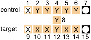
CNOT-gate
(b)	(c)
general rotation	$z$-rotation
(d)	(e)
Hadamard-gate	$\pi/2$-phase gate

Figure 1: Realization of elementary quantum gates on the $\mbox{QC}_{\cal{C}}$. Each square represents a lattice qubit. The squares in the extreme left column marked with white circles denote the input qubits, they on the right-most column denote the output qubits. Note that blank squares can represent either $\sigma_{z}$ measurements or empty lattice sites.

The measurement bases ${\cal{B}}(\varphi)$ and ${\cal{B}}(-\varphi)$ in (5) coincide for angles $\varphi=0$ and for $\varphi=\pm\pi/2$. For $\varphi=0$ the measurement basis ${\cal{B}}(\varphi)$ is the eigenbasis of $\sigma_{x}$, and for $\varphi=\pm\pi/2$ the measurement basis ${\cal{B}}(\varphi)$ is the eigenbasis of $\sigma_{y}$. In these cases, the choice of the measurement basis is not influenced by the results of measurements at other qubits. Therefore, rotations whose Euler angles $\xi,\eta,\zeta$ are in the set $\{0,\pm\pi/2\}$ can be realized simultaneously in the first round of measurements, that is no other cluster qubits need to be measured before. Among these rotations are the Hadamard gate and the $\pi/2$ phase shift. As displayed in Fig. 1, the Hadamard gate and the $\pi/2$-phase shift are both realized by performing a pattern of $\sigma_{x}$- and $\sigma_{y}$-measurements on the cluster ${\cal{C}}$. The byproduct operators which are thereby created are

$$\begin{array}[]{rcl}U_{\Sigma,H}&=&\sigma_{x}^{s_{1}+s_{3}+s_{4}+\kappa_{1,I}^{\prime}+\kappa_{3}^{\prime}+\kappa_{4}^{\prime}}\,\sigma_{z}^{s_{2}+s_{3}+\kappa_{2}^{\prime}+\kappa_{3}^{\prime}+\kappa_{5,O}^{\prime}}\\ U_{\Sigma,U_{z}(\pi/2)}&=&\sigma_{x}^{s_{2}+s_{4}+\kappa_{2}^{\prime}+\kappa_{4}^{\prime}}\,\sigma_{z}^{s_{1}+s_{2}+s_{3}+\kappa_{1,I}^{\prime}+\kappa_{2}^{\prime}+\kappa_{3}^{\prime}+\kappa_{5,O}^{\prime}}.\end{array}$$ (13)

Owing to the special Euler angles for the Hadamard- and the $\pi/2$-phase gate, the propagation relations for these rotations can also be written in a form resembling the propagation relation (12) for the CNOT-gate

$$\begin{array}[]{rcl}H\,{\sigma_{x}}^{s_{x}}{\sigma_{z}}^{s_{z}}&=&{\sigma_{x}}^{s_{z}}{\sigma_{z}}^{s_{x}}\,H,\\ U_{z}(\pi/2)\,{\sigma_{x}}^{s_{x}}{\sigma_{z}}^{s_{z}}&=&{\sigma_{x}}^{s_{x}}{\sigma_{z}}^{s_{x}+s_{z}}\,U_{z}(\pi/2).\end{array}$$ (14)

Under propagation –via the propagation relations (11), (12) and (14)– the byproduct operators resulting from the implementation of the universal gates generate a subgroup of the group

$${\cal{U}}^{\mbox{\tiny{local}}}=\left\{1,\sigma_{x}^{(i)},\sigma_{z}^{(i)},i=1..n,\;\,\mbox{and products thereof}\right\}$$ (15)

of all possible byproduct operators. ${\cal{U}}^{\mbox{\tiny{local}}}\subset SU(2)^{\otimes n}$ is a subset of the set of all multi-local unitary operations. Hence, it can be compensated for at the end of the computation by a local change of the measurement bases.

To summarize, any quantum logic network can be simulated on a one-way quantum computer. A set of universal gates can be realized by one-qubit measurements and the gates can be combined to circuits. Due to the randomness of the results of the individual measurements, unwanted byproduct operators are introduced. These byproduct operators can be accounted for by adapting measurement directions throughout the process of computation. In this way, a subset of qubits on the cluster ${\cal{C}}$ is prepared as the output register. The quantum state on this subset of qubits equals that of the quantum register of the simulated network up to the action of an accumulated byproduct operator. The byproduct operator determines how the measurements on the output register are to be interpreted.

3 Beyond the network picture

In the previous section we have described the $\mbox{QC}_{\cal{C}}\,\,$in a network terminology, which has been useful to prove the universality of the scheme. On the other hand, the cluster qubits do not have to be measured in the order prescribed by the order of the gates in the corresponding network. This observation indicates that the network picture does not describe the $\mbox{QC}_{\cal{C}}\,\,$in every respect.

3.1 The sets $Q_{t}$ of simultaneously measurable qubits

The cluster qubits which we have chosen to take the role of the readout register, for example, are just qubits like any other cluster qubits. It turns out that, in a more efficient way of running the $\mbox{QC}_{\cal{C}}$, the “readout” qubits are not the last ones to be measured but among the first. It is advantageous to forget about the network altogether and to view the $\mbox{QC}_{\cal{C}}\,\,$as a set of one-qubit measurements on a resource quantum state, the cluster state. These measurements have to be performed in a certain order and in a certain basis. The classical information of how to measure subsequent qubits must all be contained in the results of the already performed measurements. Similarly, the final result of the computation must be contained in all the measurement outcomes together.

In the following we will adopt the strategy that every cluster qubit is measured at the earliest possible time. This means that each qubit is measured as soon as the required measurement results from other qubits which determine its measurement basis are known. Let us denote by $Q_{t}$ the set of qubits which can be measured at the same time in the measurement round $t$. So, how can the sets $Q_{t}$ be determined? $Q_{0}$ is the set of qubits which are measured in the first round. These are all the qubits whose observables $\sigma_{x}$, $\sigma_{y}$ or $\sigma_{z}$ are measured. The measurement bases for these qubits do not depend on the results of any previous measurements. To determine the subsequent set $Q_{1}$, one looks at which qubits can be measured with the knowledge of the measurement results from the qubits in $Q_{0}$. Next, one looks which qubits can be measured with the measurement results from the qubits in $Q_{0}$ and $Q_{1}$ known. These qubits form the set $Q_{2}$. In this manner one proceeds until the whole cluster ${\cal{C}}$ is divided into disjoint subsets $Q_{t}$.

As will become clear later, it is useful to introduce the sets $Q^{(t)}$ of yet-to-be measured qubits. More precisely, $Q^{(t)}$ is the set of qubits which remain to be measured after measurement round No. $t-1$,

$$Q^{(t)}=\bigcup\limits_{i=t}^{t_{\mbox{\tiny{max}}}}Q_{i}.$$ (16)

Mathematically, the sets $Q_{t}$ are derived from a strict partial ordering in ${\cal{C}}$. The strict partial ordering, in turn, is generated by forward cones which are explained in the next section.

3.2 The forward- and backward cones

Be $g$ a gate in the network ${\cal{N}}$ to be simulated and $k\in{\cal{C}}(g)$ a cluster qubit that belongs to the implementation of $g$. Further, be ${\cal{O}}$, $A$ and $\Omega$ three vertical cuts through the network ${\cal{N}}$. A vertical cut is such that it intersects each qubit line in a network only once and that it does not intersect gates. ${\cal{O}}$ intersects ${\cal{N}}$ just after the gate $g$, i.e. the byproduct operator $U_{\Sigma,g}$ caused by the implementation of $g$, as given in (8) and (10), is located on ${\cal{O}}$. Note that the byproduct operators generated on ${\cal{O}}$ depend on the measurement results obtained in course of the gate implementation via ${\left(U_{k}\right)}^{s_{k}}$. $A$ intersects ${\cal{N}}$ just be fore the input, i.e. an operator propagated to $A$ acts on the input register of ${\cal{N}}$, and $\Omega$ intersects ${\cal{N}}$ just before the output such that an operator propagated to $\Omega$ acts on the output register of ${\cal{N}}$. We can now define the forward- and backward cones of the cluster qubits $k\in{\cal{C}}$.

Definition 1

The forward cone $\mbox{{\em{fc}}}(k)$ of a cluster qubit $k\in{\cal{C}}$ is the set of all those cluster qubits $j\in Q^{(1)}$ whose measurement basis ${\cal{B}}(\varphi_{j,\mbox{{\em{\footnotesize{meas}}}}})$ depends on the result $s_{k}$ of the measurement of qubit $k$ after the byproduct operator ${\left(U_{k}\right)}^{s_{k}}$ is propagated from ${\cal{O}}$ to $\Omega$.

Definition 2

The backward cone $\mbox{{\em{bc}}}(k)$ of a cluster qubit $k\in{\cal{C}}$ is the set of all those cluster qubits $j\in Q^{(1)}$ whose measurement basis ${\cal{B}}(\varphi_{j,\mbox{{\em{\footnotesize{meas}}}}})$ depends on the result $s_{k}$ of the measurement of qubit $k$ after the byproduct operator ${\left(U_{k}\right)}^{s_{k}}$ is propagated from ${\cal{O}}$ to $A$.

It will turn out that only the backward cones of the qubits $k\in Q_{0}$ constitute part of the information specifying an algorithm on the $\mbox{QC}_{\cal{C}}$, but nevertheless all the backward- and forward cones are important objects in the scheme. Either of the sets, the set of the forward- and that of the backward cones, separately contains the full information of the temporal structure of a computation on the $\mbox{QC}_{\cal{C}}$.

Let us examine the definitions 1 and 2 for a particular example, the general one-qubit rotation (3) as implemented by the procedure (6) modulo a byproduct operator $U_{\Sigma,Rot}$ as given in (8). The measurement result $s_{1}$ of qubit 1 (cf. Fig. 1) modifies the measurement angle of qubit 2, which is responsible for implementing an $x$-rotation $U_{x}(\xi)$, by a factor ${(-1)}^{s_{1}}$. Further, it causes a byproduct operator ${(\sigma_{z})}^{s_{1}}$ at ${\cal{O}}$. If this byproduct operator is propagated forward from ${\cal{O}}$ to $\Omega$ it has no effect on qubit 2, because qubit 2 is behind ${\cal{O}}$. The dependence on $s_{1}$ of the basis in which qubit 2 has to be measured persists and thus qubit 2 is in the forward cone of qubit 1, $\,\,2\in\mbox{fc}(1)$. The situation is different if the byproduct operator ${(\sigma_{z})}^{s_{1}}$ is propagated backwards from ${\cal{O}}$ to $A$: via the propagation relation (11) the Euler angle $\xi$ is modified by a factor ${(-1)}^{s_{1}}$ which has to be accounted for by multiplying the measurement angle $\varphi_{2,{\mbox{\footnotesize{meas}}}}$ by a factor ${(-1)}^{s_{1}}$, too. Thus, the factor ${(-1)}^{s_{1}}$ modifies the measurement angle $\varphi_{2,{\mbox{\footnotesize{meas}}}}$ twice, once via the procedure (6) and once in backward propagation, and there is no net effect. Qubit 2 is not in the backward cone of qubit 1, $\,\,2\not\in\mbox{bc}(1)$.

What does it mean that a cluster qubit $j$ is in the forward cone of another cluster qubit $k$, $j\in\mbox{fc}(k)$? According to the definition, a byproduct operator created via the measurement at cluster qubit $k$ influences the measurement angle $\varphi_{j,\mbox{\footnotesize{meas}}}$ at cluster qubit $j$. To determine the measurement angle at $j$ one must thus wait for the measurement result at $k$ to see what the byproduct operator created randomly by the measurement at $k$ is. If $j\in\mbox{fc}(k)$, the measurement at qubit $j$ is performed later than that at qubit $k$. This we denote by $k\prec j$

$$j\in\mbox{fc}(k)\Rightarrow k\prec j.$$ (17)

Please note that the converse of (17) is not true. If $k\prec j$ holds, still $j\in\mbox{fc}(k)$ may not. This can be easily verified for the example of a general rotation (3). There, according to the procedure for implementing such a rotation described in Section 2, the result of the measurement of qubit 1 enters into in which basis qubit 2 has to be measured. Hence, $2\in\mbox{fc}(1)$. By (17), $1\prec 2$ which means that the measurement at qubit 2 has to wait for the result of the measurement on qubit 1. Similarly, the measurement result on qubit 2 enters in the choice of the measurement basis for the measurement on qubit 3. $3\in\mbox{fc}(2)$ and thus $2\prec 3$. Then $1\prec 3$ also holds as shown below in (18) , but $3\not\in\mbox{fc}(1)$, since the measurement result on qubit 1 does not influence the choice of the measurement basis for the measurement on qubit 3.

The relation “$\prec$” is a strict partial ordering. Suppose, that besides $k\prec j$, for another cluster qubit $l$ one had $l\in\mbox{fc}(j)$ and thus $j\prec l$. This would mean that the measurement at $l$ must wait for the measurement at $j$, which itself had to wait for the measurement at $k$. Thus, the measurement at $l$ also had to wait for the measurement at $k$. Therefore the relation “$\prec$” is transitive,

$$k\prec j\,\,\wedge\,\,j\prec l\,\longrightarrow\,k\prec l.$$ (18)

Further, a measurement to implement a gate cannot and does not need to wait for its own result. Therefore the relation “$\prec$” is anti-reflexive,

$$\neg\exists j\in{\cal{C}}:j\prec j.$$ (19)

Let us now cast the procedure to construct the sets of simultaneously measured qubits given above in more precise terms. Be $Q_{t}\subset{\cal{C}}$ the set of cluster qubits measured in measurement round $t$, and $Q^{(t)}\subset{\cal{C}}$ the set of qubits which are to be measured in the measurement round $t$ and all subsequent rounds, as defined in (16). Then, $Q_{0}$ is the set of qubits which are measured in the first round. These are the qubits of which the observables $\sigma_{x}$, $\sigma_{y}$ or $\sigma_{z}$ are measured, so that the measurement bases are not influenced by other measurement results. Further, $Q^{(0)}={\cal{C}}$. Now, the sequence of sets $Q_{t}$ can be constructed using the following recursion relation

$$\begin{array}[]{lcl}Q_{t}&=&\displaystyle{\left\{q\in Q^{(t)}|\neg\exists p\in{Q}^{(t)}:p\prec q\right\}}\\ Q^{(t+1)}&=&\displaystyle{Q^{(t)}\backslash Q_{t}}.\end{array}$$ (20)

All those qubits which have no precursors in some remaining set $Q^{(t)}$ and thus do not have to wait for results of measurements of qubits in $Q^{(t)}$ are taken out of this set to form $Q_{t}$. The recursion proceeds until ${Q}^{(t_{\mbox{\footnotesize{max}}}+1)}=\emptyset$ for some maximal value $t_{\mbox{\footnotesize{max}}}$ of $t$.

Can it happen that the recursion does not terminate? That were the case if for a number $m$ of qubits $j_{1},...,j_{m}\in{\cal{C}}$ formed a cycle $j_{1}\prec j_{2}\prec...\prec j_{m}\prec j_{1}$. Then, none of the qubits $j_{1},..,j_{n}$ could ever taken out of the set. However, by transitivity (18) we then had $j_{1}\prec j_{1}$ which contradicts anti-reflexivity (19). Hence, such a situation cannot occur.

Let us at the end of this section define the forward- and backward cones $\mbox{fc}(g)$, $\mbox{bc}(g)$ of the gates $g$. In eq. (10) we have seen that the byproduct operator caused by the implementation of a CNOT-gate contains a constant contribution $U_{0}(CNOT)=\sigma_{z}^{(c)}$. This contribution to the byproduct operator does not depend on any local variables such as the measurement results and is thus attributed to the gate as a whole. This byproduct operator is of the same form as those depending on the individual measurement results and can influence measurement angles when being propagated forward or backward. Thus we define the forward- and backward cones of gates, in analogy to those of the cluster qubits $k\in{\cal{C}}$, as follows:

The forward cone $\mbox{fc}(g)$ of a gate $g\in{\cal{N}}$ is the set of all those cluster qubits $j\in Q^{(1)}$ of which the measurement basis ${\cal{B}}(\varphi_{j,\mbox{{\em{\footnotesize{meas}}}}})$ is modified if the byproduct operator $U_{0}(g)$ is propagated forward from ${\cal{O}}$ to $\Omega$.

The backward cone $\mbox{bc}(g)$ of a gate $g\in{\cal{N}}$ is the set of all those cluster qubits $j\in Q^{(1)}$ of which the measurement basis ${\cal{B}}(\varphi_{j,\mbox{{\em{\footnotesize{meas}}}}})$ is modified if the byproduct operator $U_{0}(g)$ is propagated backward from ${\cal{O}}$ to $A$.

The forward- and backward cones of gates contain some information about the temporal structure of an algorithm on the $\mbox{QC}_{\cal{C}}$, but –in contrast to the backward- and forward cones of the cluster qubits– not all. Also they do not form part of the information representing a quantum algorithm on the $\mbox{QC}_{\cal{C}}$, they will be absorbed into the algorithm angles. Their role for the description of a computation on the $\mbox{QC}_{\cal{C}}\,\,$is a technical one.

3.3 The algorithm- and measurement angles

There are three different types of angles involved in the described scheme of quantum computation of which the most prominent are the algorithm angles and the measurement angles.

The algorithm angles $\big{\{}\varphi_{j,{\mbox{\footnotesize{algo}}}},j\in Q^{(1)}\big{\}}$ are part of the information that specifies an algorithm on the $\mbox{QC}_{\cal{C}}$. They are derived from the network angles $\big{\{}\varphi_{j,\mbox{\footnotesize{qln}}},j\in Q^{(1)}\big{\}}$, i.e. the Euler angles of the one-qubit rotations in the quantum logic network. Further, the algorithm angles depend on the set $\big{\{}\kappa_{k},k\in{\cal{C}}\big{\}}$ characterizing the cluster state $|\phi\rangle_{\cal{C}}$ in (2), and on special properties of the measurement pattern. We see that the network angles are absorbed into the algorithm angles. They do not constitute part of the information specifying a $\mbox{QC}_{\cal{C}}$-algorithm.

As described before, the process of computation with the $\mbox{QC}_{\cal{C}}\,\,$comprises several measurement rounds. The first round, in wich the qubits in the set $Q_{0}$ are measured, is somewhat different from the following rounds. Therein, all gates of the circuit that belong to the Clifford group are implemented at the same time, no matter where they are located in the corresponding quantum logic network and in which step they would be carried out there. This results in byproduct operators scattered all over the place. These byproduct operators are, according to the scheme described in Section 4.2, propagated backwards. To account for the effect that the byproduct operators have on the algorithm angles, these angles have to updated to the modified algorithm angles $\big{\{}\varphi_{j,{\mbox{\footnotesize{algo}}}}^{\prime},j\in Q^{(1)}\big{\}}$. The modified algorithm angles $\varphi_{j,{\mbox{\footnotesize{algo}}}}^{\prime}$ are calculated from the respective algorithm angles $\varphi_{j,{\mbox{\footnotesize{algo}}}}$ and the results obtained in the first measurement round $\big{\{}s_{k},k\in Q_{0}\big{\}}$. In the subsequent measurement rounds no further update of the modified algorithm angles occurs. Finally, each qubit $j\in Q_{t}\subset Q^{(1)}$ is measured in some measurement round $t$ in the basis ${\cal{B}}(\varphi_{j,{\mbox{\footnotesize{meas}}}})$ where $\varphi_{j,{\mbox{\footnotesize{meas}}}}$ denotes the measurement angle of qubit $j$. The measurement angle $\varphi_{j,{\mbox{\footnotesize{meas}}}}$ of a qubit $j\in Q_{t}$ is calculated from the modified algorithm angle, $\varphi_{j,{\mbox{\footnotesize{algo}}}}^{\prime}$ and the results $\big{\{}s_{k},k\in\bigcup_{i=0}^{t-1}Q_{i}\big{\}}$ of the so far obtained measurements.

Before a quantum algorithm is run on the $\mbox{QC}_{\cal{C}}$, the algorithm angles are determined from the cluster and the properties of the algorithm. During runtime of the $\mbox{QC}_{\cal{C}}$, in the first measurement round $(t=0)$, the algorithm angles are replaced by the modified algorithm angles, i.e. only the latter are kept while the former are erased. Then, in the measurement round $t$ a qubit $j\in Q_{t}$ is measured in the basis determined by the measurement angle $\varphi_{j,{\mbox{\footnotesize{meas}}}}$. After the measurement of qubit $j$ both $\varphi_{j,{\mbox{\footnotesize{algo}}}}^{\prime}$ and $\varphi_{j,{\mbox{\footnotesize{meas}}}}$ can be erased.

Now there arises the question of how the measurement angles of the actual measurements are calculated from the results of previous measurements. This question will be answered in Section 4.2. The question which interests us most, of course, is: “How can the final result of the computation be determined from all the measurement outcomes?” It will turn out that the answers to both questions are very much related.

3.4 Quantities for the processing of the measurement results

3.4.1 The information vector

Let us again –as in Section 3.1– make the change of the viewpoint from an explanation of the $\mbox{QC}_{\cal{C}}\,\,$within the network model to a more suitable description, but now focusing on the quantities required to describe the processing of the measurement results.

Suppose in the simulation of a quantum logic network ${\cal{N}}$ on the $\mbox{QC}_{\cal{C}}\,\,$in a network manner –i.e. measuring the “readout” qubits at last– the processing has reached the stage where all but those cluster qubits have been measured which form the output register.

The accumulated byproduct operator $U_{\Sigma}$ to act upon the logical output qubits $1,..,n$ is known. It has the form

$$U_{\Sigma}=\prod\limits_{i=1}^{n}\,\,{\left(\sigma_{x}^{(i)}\right)}^{x_{i}}{\left(\sigma_{z}^{(i)}\right)}^{z_{i}},$$ (21)

where $x_{i},z_{i}\in\{0,1\}$ for $1\leq i\leq n$. Let us now label the unmeasured qubits on the cluster in the same way as the readout qubits on the quantum logic network are labelled.

The “readout” qubits on the cluster are, at this point, in a state $U_{\Sigma}|\mbox{out}\rangle$, where $|\mbox{out}\rangle$ is the output state of the corresponding quantum logic network. In the network picture, the computation is completed by measuring each qubit in the $\sigma_{z}$-eigenbasis, thereby obtaining the measurement results $\{s_{i}^{\prime}\}$, say. In the $\mbox{QC}_{\cal{C}}\,\,$scheme, one measures the state $U_{\Sigma}|\mbox{out}\rangle$ directly, whereby outcomes $\{s_{i}\}$ are obtained and the “readout” qubits are projected into the state $|{\cal{M}}\rangle=\prod_{i=1}^{n}\frac{1+{(-1)}^{s_{i}}\sigma_{z}^{(i)}}{2}\,\,U_{\Sigma}|\mbox{out}\rangle$. Depending on the known byproduct operator $U_{\Sigma}$, the set of measurement results $\{s_{i}\}$ in general has a different interpretation from what the network readout $\{s_{i}^{\prime}\}$ would have. The measurement basis is the same. From (21) one obtains

$$\begin{array}[]{rcl}|{\cal{M}}\rangle=\prod_{i=1}^{n}\frac{1+{(-1)}^{s_{i}}\sigma_{z}^{(i)}}{2}\,U_{\Sigma}|\mbox{out}\rangle&=&U_{\Sigma}\left(U_{\Sigma}^{\dagger}\,\prod_{i=1}^{n}\frac{1+{(-1)}^{s_{i}}\sigma_{z}^{(i)}}{2}U_{\Sigma}\right)|\mbox{out}\rangle\\ &=&U_{\Sigma}\,\prod_{i=1}^{n}\frac{1+{(-1)}^{s_{i}+x_{i}}\sigma_{z}^{(i)}}{2}|\mbox{out}\rangle\end{array}$$ (22)

From (22) we see that a $\sigma_{z}$-measurement on the state $U_{\Sigma}\,|\mbox{out}\rangle$ with results $\{s_{i}\}$ represents the same algorithmic output as a $\sigma_{z}$-measurement of the state $|\mbox{out}\rangle$ with the results $\{s_{i}^{\prime}\}$, where the sets $\{s_{i}\}$ and $\{s_{i}^{\prime}\}$ are related by

$$s_{i}^{\prime}\equiv s_{i}+x_{i}\;\mbox{mod}\,\,2.$$ (23)

The set $\{s_{i}^{\prime}\}$ represents the result of the computation. It can be calculated from the results $\{s_{i}\}$ of the $\sigma_{z}$-measurements on the “readout” cluster qubits, and the values $\{x_{i}\}$ which can be extracted from the byproduct operator $U_{\Sigma}$. We see that both the contribution of the byproduct operator and the result of the measurement on the “readout” qubits of the cluster enter expression (23) in the same way. Indeed, there is no need to distinguish between these two contributions. On the level of the byproduct operators, the readout measurement result is translated into an additional contribution to the accumulated byproduct operator. Both contributions to the such extended byproduct operator

$$U_{\Sigma R}=U_{\Sigma}U_{R},\;\mbox{with}\;U_{R}=\prod_{i=1}^{n}{(\sigma_{x}^{(i)})}^{s_{i}},$$ (24)

stem from random measurement results. It is just that the contributions which constitute $U_{\Sigma}$ must be propagated forward from where they originated and the additional contributions from the readout measurements must be propagated one step backwards. Both the forward and the backward propagated contributions to $U_{\Sigma R}$ are propagated to the same location in the network. Forward and backward propagation are closely related. In fact, as the propagation relations (11), (12) and (14) are their own inverse, the rules are the same for both directions. The distinguished role of the readout qubits is only a remnant of the interpretation of the $\mbox{QC}_{\cal{C}}\,\,$as a quantum logic network. A more adequate description will have the consequence that the cluster qubits on the “output register”, for instance, will be measured during the initialization of the $\mbox{QC}_{\cal{C}}\,\,$such that they are removed from the entangled quantum state even before the main part of the computation starts.

We now define the the information vector ${\bf{I}}$, a $2n$-component binary vector which is a function of the quantities $\{x_{i},z_{i}\}$ and the results $\{s_{i}\}$ of the measurements on the cluster output register. Together, these quantities determine the extended byproduct operator $U_{\Sigma R}$ via (21), and(24).

Definition 3

The information vector ${\bf{I}}$ is given by

$${\bf{I}}=\left(\begin{array}[]{c}\mbox{ }\\ {\bf{I}}_{x}\\ \vspace*{0.3cm}\hfil\\ {\bf{I}}_{z}\\ \mbox{ }\end{array}\right),\;\;\;\mbox{with}\;\;{\bf{I}}_{x}=\left(\begin{array}[]{c}x_{1}+s_{1}\\ x_{2}+s_{2}\\ .\\ .\\ .\\ x_{n}+s_{n}\end{array}\right),\;\;\;{\bf{I}}_{z}=\left(\begin{array}[]{c}z_{1}\\ z_{2}\\ .\\ .\\ .\\ z_{n}\end{array}\right).$$ (25)

As can be seen from (23) and (25), ${\bf{I}}_{x}$ is a possible result of a readout measurement in a corresponding quantum logic network. ${\bf{I}}_{z}$ is redundant. However, in Section 4.1 the flow quantity ${\bf{I}}(t)$, the information flow vector, will be defined for which ${\bf{I}}(t_{\mbox{\footnotesize{max}}})={\bf{I}}$, with $t_{\mbox{\footnotesize{max}}}$ the index of the final computational step. For $t<t_{\mbox{\footnotesize{max}}}$, in ${\bf{I}}(t)$ both the $z$-part ${\bf{I}}_{z}(t)$ and the $x$-part ${\bf{I}}_{x}(t)$ are required to determine the bases for the one-qubit measurements in $Q_{t+1}$. As ${\bf{I}}_{z}(t)$ is of equal importance as ${\bf{I}}_{x}(t)$ throughout the process of computation we keep ${\bf{I}}_{z}$ in the definition of ${\bf{I}}$ as well.

The set of possible information vectors ${\bf{I}}$ forms a $2n$ dimensional vector space over $F_{2}$, ${\cal{V}}$. Let us consider the group ${\cal{U}}^{\mbox{\tiny{local}}}$ of all possible extended byproduct operators $U_{\Sigma R}$. If we divide out the normal divisor $\{\pm 1\}$ of ${\cal{U}}^{\mbox{\tiny{local}}}$, the resulting factor group $\overline{\cal{U}}={\cal{U}}^{\mbox{\tiny{local}}}/\{\pm 1\}$ is isomorphic to ${\cal{V}}$. From the viewpoint of physics, dividing out the normal divisor $\{\pm 1\}$ means that we ignore a global phase. The isomorphism ${\cal{I}}$ which maps an ${\bf{I}}\in{\cal{V}}$ to the corresponding $U_{\Sigma R}\in\overline{\cal{U}}$ is given by

$${\cal{I}}:\,\,{\cal{V}}\ni{\bf{I}}\longrightarrow U_{\Sigma R}=\prod\limits_{i=1}^{n}\,\,{\left(\sigma_{x}^{(i)}\right)}^{{[I_{x}]}_{i}}{\left(\sigma_{z}^{(i)}\right)}^{{[I_{z}]}_{i}}\in\overline{\cal{U}},$$ (26)

where ${[I_{x}]}_{i}$ and ${[I_{z}]}_{i}$ are the respective components of ${\bf{I}}_{x}$ and ${\bf{I}}_{z}$. The component-wise addition of vectors in ${\cal{V}}$ corresponds, via the isomorphism ${\cal{I}}$, to the multiplication of byproduct operators modulo a phase factor $\{\pm 1\}$. The procedure to implement this product is to first use the operator product, then bring the factors into normal order according to (26) and finally drop the phase. Multiplication of vectors ${\bf{I}}\in{\cal{V}}$ with the scalars 0,1 corresponds to raising the byproduct operators $U_{\Sigma R}\in\overline{\cal{U}}$ to the respective powers. One may switch between the two pictures via the isomorphism (26). The algebraic structures involved will be more apparent in the representation using the information vector ${\bf{I}}={\bf{I}}\left(\{x_{i},z_{i},s_{i}\}\right)$ than in the formulation of the operator $U_{\Sigma R}$.

Now that we have defined the information vector ${\bf{I}}$ in (25) and have seen that the result of the computation can be directly read off from the $x$-part of ${\bf{I}}$, we would like to find out how ${\bf{I}}$ depends on the measurement outcomes $\big{\{}s_{k}\big{\}}$ and the set $\big{\{}\kappa_{k}\big{\}}$ of binary numbers that determine the cluster state $|\phi\rangle_{\cal{C}}$ in (2). This task is left until Section 4.1. Before we can accomplish it we need some further definitions. It will turn out that the information vector ${\bf{I}}$ can be written as a linear combination of the byproduct images which are explained next.

3.4.2 The byproduct images

Be $\Omega$ the “cut” through a network ${\cal{N}}$ which intersects the qubit lines just before its output. This is the cut at which the extended byproduct operator $U_{\Sigma R}$ is accumulated. Consider a qubit $k$ on the cluster ${\cal{C}}$ which is measured in the course of computation. Depending on the result of the measurement on qubit $k$, a byproduct operator ${\left(U_{k}\right)}^{s_{k}}$ is introduced in ${\cal{N}}$ at the location of the logical output qubits of the gate for whose implementation the cluster qubit $k$ was measured. This byproduct operator $U_{k}$ can –by using the propagation relations (11), (12) and (14)– propagated from where it occurred to the cut $\Omega$. There it appears as the forward propagated byproduct operator $U_{k}|_{\Omega}$. Now we can define the byproduct image ${\bf{F}}_{k}$ of a cluster qubit $k\in{\cal{C}}$.

Definition 4

Each cluster qubit $k\in{\cal{C}}$ has a byproduct image ${\bf{F}}_{k}$, which is the vector that corresponds via the isomorphism ${\cal{I}}^{-1}$ (26) to the forward propagated byproduct operator $U_{k}|_{\Omega}$,

$${\bf{F}}_{k}={\cal{I}}^{-1}\left(U_{k}|_{\Omega}\right).$$ (27)

In the definition (27) of the byproduct image ${\bf{F}}_{k}$ it is mentioned only implicitly that the image is evaluated on the cut $\Omega$. Later in the discussion it will become apparent that we could evaluate the byproduct image on every vertical cut ${\cal{O}}$. Sometimes, if we compare to other vertical cuts, we will explicitly write ${\bf{F}}_{k}|_{\Omega}$ for ${\bf{F}}_{k}$.

The set of byproduct images $\left\{{\bf{F}}_{k},k\in{\cal{C}}\right\}$ is an important quantity for the scheme. It represents part of the information which is needed to run a quantum algorithm with the $\mbox{QC}_{\cal{C}}$.

In eq. (10) the byproduct operator for the CNOT-gate as realized according to Fig. 1 is given. This byproduct operator contains a constant contribution $U_{0}(CNOT)=\sigma_{z}^{(c)}$. As $U_{0}$ does not depend on any local variables, neither on $\big{\{}s_{k}\big{\}}$ nor on $\big{\{}\kappa_{k}\big{\}}$, it makes no sense to attribute it to any of the cluster qubits that were measured to realize the gate. Instead, it is attributed to the part of the measurement pattern that implements the gate as a whole, or –for simplicity– to the gate itself. For any gate $g$, $U_{0}(g)$ can be propagated forward to the cut $\Omega$ to act upon the “readout” qubits. There it appears as the forward propagated byproduct operator $U_{0}(g)|_{\Omega}$. In analogy to the byproduct images of the cluster qubits, we can now define the byproduct images of the gates $g$ of the quantum logic network that is simulated on the $\mbox{QC}_{\cal{C}}$. For any such gate $g$ the byproduct image ${\bf{F}}_{g}$ is the vector that corresponds to $U_{0}(g)|_{\Omega}$ via

$${\bf{F}}_{g}={\cal{I}}^{-1}(U_{0}(g)|_{\Omega}).$$ (28)

Please note that in contrast to the byproduct images ${\bf{F}}_{k}$ of cluster qubits $k\in{\cal{C}}$ the byproduct images ${\bf{F}}_{g}$ of gates do not form a separate part of the information specifying a quantum algorithm on the $\mbox{QC}_{\cal{C}}$. They will be absorbed into the initialization value ${\bf{I}}_{\mbox{\footnotesize{init}}}$ of the information flow vector defined in Section 4.1 and they are thus only a convenient tool in the derivation of the computational model.

Via ${\cal{I}}^{-1}$ we map the multiplication of byproduct operators, i.e. their accumulation, onto addition modulo 2 on the level of the vectors in ${\cal{V}}$. Now there arises the question whether other operations on the byproduct operators could be expressed in terms of the corresponding vectors, too. Specifically, one may ask how the byproduct operator propagation looks like on the level of the ${\bf{I}}\in{\cal{V}}$.

3.4.3 The propagation matrices

The answer to this question is that on the level of the vector quantities in ${\cal{V}}$ propagation is described by multiplication with certain $2n\times 2n$-matrices $C$. Consider two cuts ${\cal{O}}_{1}$ and ${\cal{O}}_{2}$ through a network which intersect each qubit line only once. Further, be the two cuts such that they do not intersect each other and that ${\cal{O}}_{1}$ is earlier than ${\cal{O}}_{2}$. The part of the quantum logic network between ${\cal{O}}_{1}$ and ${\cal{O}}_{2}$ is denoted by ${\cal{N}}_{{\cal{O}}_{1}\rightarrow{\cal{O}}_{2}}$. Be ${\bf{I}}_{k}|_{{\cal{O}}_{1}}$ and ${\bf{I}}_{k}|_{{\cal{O}}_{2}}$ the vectors describing a byproduct operator resulting from the measurement of qubit $k$, propagated to the cuts ${\cal{O}}_{1}$ and ${\cal{O}}_{2}$, respectively. Then we have

$${\bf{I}}_{k}|_{{\cal{O}}_{2}}=C({{\cal{N}}_{{\cal{O}}_{1}\rightarrow{\cal{O}}_{2}}})\,{\bf{I}}_{k}|_{{\cal{O}}_{1}}.$$ (29)

To any quantum logic network ${\cal{N}}$ a matrix $C_{\cal{N}}$ can be assigned. For a network ${\cal{N}}_{2}\circ{\cal{N}}_{1}$ composed of two subnetworks ${\cal{N}}_{1}$ and ${\cal{N}}_{2}$ (of which ${\cal{N}}_{1}$ is carried out first) the propagation matrix is equal to the product of the propagation matrices of the subnetworks

$$C({{\cal{N}}_{2}\circ{\cal{N}}_{1}})=C({{\cal{N}}_{2}})C({{\cal{N}}_{1}}).$$ (30)

Because of property (30) we only need to find the propagation matrices for the general one-qubit rotations, the CNOT-, the Hadamard- and the $\pi/2$-phase gate. The one-qubit rotations and the CNOT-gate alone form a universal set of gates. The reason why we also include the Hadamard- and the $\pi/2$-phase gate is that here they are treated differently from the general rotations, as can be seen from the propagation relations (11) and (14). By propagation through a Hadamard- or $\pi/2$-phase gate, the gate is left unchanged while the byproduct operator changes; whereas for the propagation through a general rotation, the rotation changes and the byproduct operator stays the same. Thus, for finding the byproduct images the general rotations in ${\cal{N}}$ can be replaced by the identity. Only the CNOT-, Hadamard and $\pi/2$-phase gates have an effect. The special treatment of the Hadamard and the $\pi/2$-phase gate is advantageous with respect to the temporal complexity of a computation, because if one uses the propagation relation (14) the implementation of the Hadamard- and the $\pi/2$-phase gate does not need to wait for results of any previous measurements. To sum up, to each possible ${\cal{N}}$ belongs a unitary operation $U({\cal{N}})$ in the Clifford group and a corresponding matrix $C({\cal{N}})$, such that

$${\cal{I}}\left({C({\cal{N}}){\bf{I}}}\right)=U({\cal{N}})\,{\cal{I}}\left({\bf{I}}\right)\,U({\cal{N}})^{\dagger}\,,\;\;\;\;\forall{\bf{I}}\in{\cal{V}}.$$ (31)

Let us now give the propagation matrices for propagation through CNOT-, Hadamard and $\pi/2$-phase gates. The propagation matrices $C$ are conveniently written in block form

$$C=\left(\begin{array}[]{ccc|ccc}&\mbox{ }&&\mbox{ }&\\ &C_{xx}&&&C_{zx}&\\ &\mbox{ }&&&\\ \hline\cr&\mbox{ }&&&\\ &C_{xz}&&&C_{zz}&\\ &\mbox{ }&&&\end{array}\right),$$ (32)

where $C_{xx}$, $C_{zx}$, $C_{xz}$ and $C_{zz}$ are $n\times n$ matrices with binary-valued entries.

For the Hadamard gate $H^{(i)}$ on the logical qubit $i$ one finds

$$\begin{array}[]{rcl}{\left[C_{xx}(H^{(i)})\right]}_{kl}={\left[C_{zz}(H^{(i)})\right]}_{kl}&=&\delta_{kl}+\delta_{ki}\delta_{il},\\ {\left[C_{zx}(H^{(i)})\right]}_{kl}={\left[C_{xz}(H^{(i)})\right]}_{kl}&=&\delta_{ki}\delta_{il},\end{array}$$ (33)

where e.g. ${\left[C_{xx}(H^{(i)})\right]}_{kl}$ denotes the entry of row $k$ and column $l$ in $C_{xx}$. Note that the qubit index $i$ is not summed over in (33) and that the addition is modulo 2.

For the $\pi/2$-phase gate $U_{z}^{(i)}(\pi/2)$ on the logical qubit $i$ one finds

$$\begin{array}[]{rcl}{\left[C_{xx}(U_{z}^{(i)}(\pi/2))\right]}_{kl}&=&\delta_{kl},\\ {\left[C_{zz}(U_{z}^{(i)}(\pi/2))\right]}_{kl}&=&\delta_{kl},\\ {\left[C_{xz}(U_{z}^{(i)}(\pi/2))\right]}_{kl}&=&\delta_{ki}\delta_{il},\\ {\left[C_{zx}(U_{z}^{(i)}(\pi/2))\right]}_{kl}&=&0.\end{array}$$ (34)

For the CNOT-gate on control qubit $c$ and target qubit $t$ one finds the propagation matrix $C(\mbox{CNOT}(c,t))$ with

$$\begin{array}[]{rcl}{\left[C_{xx}(\mbox{CNOT}(c,t))\right]}_{kl}&=&\delta_{kl}+\delta_{kt}\delta_{cl},\\ {\left[C_{zz}(\mbox{CNOT}(c,t))\right]}_{kl}&=&\delta_{kl}+\delta_{kc}\delta_{tl},\\ C_{zx}(\mbox{CNOT}(c,t))&=&0,\\ C_{xz}(\mbox{CNOT}(c,t))&=&0.\end{array}$$ (35)

We will make use of the propagation matrices in the discussion of temporal complexity of algorithms on the $\mbox{QC}_{\cal{C}}\,\,$in Section 5.2.

For the action of the propagation matrices $C$ on the vectors ${\bf{I}}\in{\cal{V}}$ there exist conserved quantities. One of them, ${\bf{I}}_{x,1}^{T}{\bf{I}}_{z,2}+{\bf{I}}_{z,1}^{T}{\bf{I}}_{x,2}$, is discussed in the next section.

3.4.4 Conservation of the symplectic scalar product

The symplectic scalar product

$$({\bf{I}}_{1},{\bf{I}}_{2})_{S}={\bf{I}}^{T}_{x,1}{\bf{I}}_{z,2}+{\bf{I}}^{T}_{z,1}{\bf{I}}_{x,2}\;{\mbox{\small{mod}}}\;2$$ (36)

is conserved. For any ${\bf{I}}_{1},{\bf{I}}_{2}\in{\cal{V}}$ and $C$ the identity

$$\left({\bf{I}}_{1},{\bf{I}}_{2}\right)_{S}=\left(C{\bf{I}}_{1},C{\bf{I}}_{2}\right)_{S}$$ (37)

holds. Let us briefly explain why the symplectic scalar product (36) is conserved. First, note that the symplectic scalar product tells whether two operators ${\cal{I}}({\bf{I}}_{1})$, ${\cal{I}}({\bf{I}}_{2})$ in the Pauli group commute or anti-commute,

$${\cal{I}}({\bf{I}}_{1}){\cal{I}}({\bf{I}}_{2})={(-1)}^{{({\bf{I}}_{1},{\bf{I}}_{2})}_{\!S}}{\cal{I}}({\bf{I}}_{2}){\cal{I}}({\bf{I}}_{1}).$$ (38)

Relation (38) is the only place in this paper where we pay attention to the sign factor of a byproduct operator. There, the product, e.g. ${\cal{I}}({\bf{I}}_{1}){\cal{I}}({\bf{I}}_{2})$, denotes the usual operator product. However, everywhere else in this paper a product ${\cal{I}}({\bf{I}}_{1}){\cal{I}}({\bf{I}}_{2})$ denotes operator multiplication modulo a global phase factor $\pm 1$, i.e. the product is normal ordered as in (26) and the phase factor is dropped.

Using relation (38), the invariance (37) of the scalar product (36) is easily demonstrated. Consider the quantity ${\cal{I}}(C{\bf{I}}_{1}){\cal{I}}(C{\bf{I}}_{2})$ with ${\cal{I}}(C{\bf{I}}_{1})=U\,{\cal{I}}({\bf{I}}_{1})\,U^{\dagger}$ and ${\cal{I}}(C{\bf{I}}_{2})=U\,{\cal{I}}({\bf{I}}_{2})\,U^{\dagger}$ as in (31). Then, we find

$$\begin{array}[]{rcl}{\cal{I}}(C{\bf{I}}_{1}){\cal{I}}(C{\bf{I}}_{2})&=&U\,{\cal{I}}({\bf{I}}_{1})\,U^{\dagger}\,U\,{\cal{I}}({\bf{I}}_{2})\,U^{\dagger}\\ &=&U\,{\cal{I}}({\bf{I}}_{1})\,{\cal{I}}({\bf{I}}_{2})\,U^{\dagger}\\ &=&{(-1)}^{{({\bf{I}}_{1},{\bf{I}}_{2})}_{\!S}}U\,{\cal{I}}({\bf{I}}_{2})\,{\cal{I}}({\bf{I}}_{1})\,U^{\dagger}\\ &=&{(-1)}^{{({\bf{I}}_{1},{\bf{I}}_{2})}_{\!S}}U\,{\cal{I}}({\bf{I}}_{2})\,U^{\dagger}\,U\,{\cal{I}}({\bf{I}}_{1})\,U^{\dagger}\\ &=&{(-1)}^{{({\bf{I}}_{1},{\bf{I}}_{2})}_{\!S}}{\cal{I}}(C{\bf{I}}_{2}){\cal{I}}(C{\bf{I}}_{1}),\end{array}$$ (39)

where the third line holds by (38). On the other hand, as we can see from (38) directly that

$${\cal{I}}(C{\bf{I}}_{1}){\cal{I}}(C{\bf{I}}_{2})={(-1)}^{{(C{\bf{I}}_{1},C{\bf{I}}_{2})}_{\!S}}{\cal{I}}(C{\bf{I}}_{2}){\cal{I}}(C{\bf{I}}_{1}).$$ (40)

From (39) and (40) together it follows that $\left({\bf{I}}_{1},{\bf{I}}_{2}\right)_{S}=\left(C{\bf{I}}_{1},C{\bf{I}}_{2}\right)_{S}$, as stated in (37).

The symplectic scalar product (36) will prove useful in determining the measurement angles from previously obtained measurement results.

3.4.5 The cone test

The cone test is used to find out whether two measurements, which are part of some gates of a circuit, influence each other, i.e. whether one of the measurements has to wait for the result of the other. The cone test does not reveal which of the two measurements has to be performed first.

Let $j,k$ be some cluster qubits $k\in{\cal{C}}$ and $j\in Q^{(1)}$. Qubit $j$ is not measured in the first measurement round and thus the observable measured at qubit $j$ is a nontrivial linear combination of $\sigma_{x}$ and $\sigma_{y}$, hence $j$ can be in the forward and backward cones of some other cluster qubits. We would like to find out whether $j$ is in the forward or backward cone of $k$. For this question the cone test provides a necessary and sufficient criterion. It reads

$$\forall\;k\in{\cal{C}},j\in Q^{(1)}:\;\;j\in\mbox{fc}(k)\vee j\in\mbox{bc}(k)\Longleftrightarrow({\bf{F}}_{j},{\bf{F}}_{k})_{S}=1.$$ (41)

To check whether a qubit lies in some other qubits backward or forward cone we only need the two forward images and can use the symplectic scalar product.

We further observe that

$$\forall\;j,k\in Q^{(1)}:\;\;j\in\mbox{fc}(k)\Longleftrightarrow k\in\mbox{bc}(j).$$ (42)

If we confine $k$ to $k\in Q^{(1)}\subset{\cal{C}}$ we can insert (42) into (41) such that the expression on the l.h.s. of (41) becomes symmetric with respect to $j$ and $k$. This fits in well since the r.h.s of (41) is also symmetric.

Similar to (41) we can give a criterion for whether or not a qubit $j\in Q^{(1)}$ is in the forward- or backward cone $\mbox{fc}(g)$, $\mbox{bc}(g)$ of some gate $g$. It reads

$$\forall g\in{\cal{N}},\,\,j\in Q^{(1)}:\;j\in\mbox{fc}(g)\vee j\in\mbox{bc}(g)\Longleftrightarrow({\bf{F}}_{j},{\bf{F}}_{g})_{S}=1.$$ (43)

The proofs of the cone tests (41), (43) and the forward-backward cone relation (42) are given in appendix A.

3.5 To what a quantum logic network condenses

Simulating a quantum logic network on a $\mbox{QC}_{\cal{C}}\,\,$is a two-stage process. Before the genuine computation, we feed a classical computer with the network to be simulated. It returns the quantities needed to run the respective algorithm on the $\mbox{QC}_{\cal{C}}$. These quantities are the sets $Q_{t}$ of simultaneously measurable qubits, the measurement bases of the qubits $k\in Q_{0}$, the algorithm angles $\varphi_{l,\mbox{\footnotesize{algo}}}$ for $l\in{\cal{C}}\backslash Q_{0}$, the backward cones $\mbox{bc}(k)$ of the qubits $k\in Q_{0}$, the byproduct images ${\bf{F}}_{j}$ for $j\in{\cal{C}}$ and the initialization value ${\bf{I}}_{\mbox{\footnotesize{init}}}$ of the information flow vector ${\bf{I}}(t)$. Together these quantities represent the program for the $\mbox{QC}_{\cal{C}}$.

In [10] we wrote that the set of one-qubit measurements on a cluster state represents the program. Now we can be more specific about the measurement pattern representing the program for the $\mbox{QC}_{\cal{C}}$. The measurement pattern has both a temporal and a spatial structure. The temporal structure is given by the sets $Q_{t}$ of simultaneously measured qubits. The spatial structure consists of the bases ($\sigma_{x}$-, $\sigma_{y}$- or $\sigma_{z}$-) of the measurements in the first round and of the measurement angles in the subsequent rounds. The measurement angles can be determined only run-time, since they involve the random outcomes of previous measurements. The measurement angles are determined using the algorithm angles and the byproduct images.

4 Computational model for the $\mbox{QC}_{\cal{C}}\,\,$

In the preceding two sections we have established the notions of the sets of simultaneously measurable qubits, backward cones, byproduct images, measurement angles and the information vector. In this section, the computational model underlying the $\mbox{QC}_{\cal{C}}\,\,$is described in these terms. First, we would like to give a summary of the characteristic features of the model:

• The $\mbox{QC}_{\cal{C}}\,\,$has no quantum input and no quantum output.

• For any given quantum algorithm, the cluster ${\cal{C}}$ is divided into disjoint subsets $Q_{t}\subset{\cal{C}}$ of qubits, $t=0,1,\dots,t_{\mbox{\footnotesize{max}}}$, where $Q_{p}\cap Q_{q}=\emptyset$ for $p\neq q$ and $\bigcup_{t=0}^{t_{\mbox{\tiny{max}}}}Q_{t}={\cal{C}}$. These subsets are measured one after the other in the order given by the index $t$. In measurement round $t$ the set $Q_{t}$ of qubits is measured.

• The classical information gained by the measurements is processed within a flow scheme. The flow quantity is a classical $2n$-component binary vector ${\bf{I}}(t)$, where $n$ is the number of logical qubits of a corresponding quantum logic network and $t$ the number of the measurement round.

• This vector ${\bf{I}}(t)$, the information flow vector, is updated after every measurement round. That is, after the one-qubit measurements of all qubits of a set $Q_{t}$ have been performed simultaneously, ${\bf{I}}(t-1$) is updated to ${\bf{I}}(t)$ through the results of these measurements. In turn, ${\bf{I}}(t)$ determines which one-qubit observables are to be measured of the qubits of the set $Q_{t+1}$.

• The result of the computation is given by the information flow vector ${\bf{I}}(t_{\mbox{\footnotesize{max}}})$ after the last measurement round. From this quantity the readout measurement result of the quantum register in the corresponding quantum logic network can be read off directly without further processing.

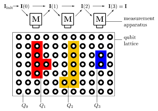
Figure 2: General scheme of the quantum computer via one-qubit measurements. The sets $Q_{t}$ of lattice qubits are measured one after the other. The results of earlier measurements determine the measurement bases of later ones. All classical information from the measurement results needed to steer the $\mbox{QC}_{\cal{C}}\,\,$is contained in the information flow vector ${\bf{I}}(t)$. After the last measurement round $t_{\mbox{\footnotesize{max}}}$, ${\bf{I}}(t_{\mbox{\footnotesize{max}}})$ contains the result of the computation.

We should make a comment on the first point. The $\mbox{QC}_{\cal{C}}\,\,$has no quantum output. Of course, the final result of any computation –including quantum computations– is a classical number, but for the quantum logic network the state of the output register before the readout measurements plays a distinguished role. For the $\mbox{QC}_{\cal{C}}\,\,$this is not the case, there are just cluster qubits measured in a certain order and basis. If, to perform a particular algorithm on the $\mbox{QC}_{\cal{C}}$, a quantum logic network is implemented on a cluster state there is a subset of cluster qubits which play the role of the output register. These qubits are, however, not the final qubits to be measured, but among the first (!).

The $\mbox{QC}_{\cal{C}}\,\,$has no quantum input. This means that the quantum input state is known and can thus be created from some standard quantum state, e.g. $|00...0\rangle$, by a circuit preceding the main part of the computation. Shor’s algorithm where one starts with an input state $\bigotimes_{i=1}^{n}1/\sqrt{2}(|0\rangle_{i}+|1\rangle_{i})$ is an example for such a situation. Other scenarios are conceivable, e.g. where an unknown quantum input is processed and the classical result of the computation is retransmitted to the sender of the input state; or the unmeasured network output register state is retransmitted. These scenarios would lead only to slight modifications in the computational model. They are, however, not in the focus of this paper. The reader who is interested in how to read in and process an unknown quantum state with the $\mbox{QC}_{\cal{C}}\,\,$is referred to [10].

4.1 Obtaining the computational result from the measurement outcomes

Now that we have defined the information vector ${\bf{I}}$ in (25) and have seen that the result of the computation can be directly read off from the $x$-part of ${\bf{I}}$, we will explain how ${\bf{I}}$ depends on the measurement outcomes $\big{\{}s_{k}\big{\}}$ and the set $\big{\{}\kappa_{k}\big{\}}$ of binary numbers that determine the cluster state $|\phi\rangle_{\cal{C}}$ in (2). For this purpose, we will express $U_{\Sigma R}$ in terms of $\big{\{}s_{k}\big{\}}$ and $\big{\{}\kappa_{k}\big{\}}$, and use the isomorphism (26) to obtain ${\bf{I}}$. As in (24), $U_{\Sigma R}$ can be decomposed into two parts, the accumulated byproduct operator $U_{\Sigma}$ and the contribution from the “readout” measurements, $U_{R}$. We will proceed in three steps. First, we will consider $U_{\Sigma}$ for the case where only the cluster qubits for the “readout” and those of which observables $\mbox{cos}\varphi\,\sigma_{x}+\mbox{sin}\varphi\,\sigma_{y}$ are measured are present. Second, we will extend the obtained result to the case where both the relevant and the redundant qubits are present, i.e. where a universal cluster ${\cal{C}}$ is used for computation. Third, we will include the contribution $U_{R}$ from the “readout” qubits.

To derive ${\bf{I}}$ as a function of $\big{\{}s_{k}\big{\}}$ and $\big{\{}\kappa_{k}\big{\}}$, we need to define the following sets. ${\cal{C}}$ is a universal cluster. Let $O\subset{\cal{C}}$ be the subset of the cluster which, in the simulation of a quantum logic network on the $\mbox{QC}_{\cal{C}}$, consists of the readout qubits. Let ${\cal{C}}_{N}\subset{\cal{C}}$ denote the cluster that contains only the relevant cluster qubits, i.e. those which are measured in a direction in the equator of the Bloch sphere, and the “readout” qubits. Be $Q_{0,z}\subset{\cal{C}}$ the set of qubits of which the operator $\sigma_{z}$ is measured. Among these sets, the following relations hold:

$$\begin{array}[]{rcl}{\cal{C}}_{N}\cup Q_{0,z}&=&{\cal{C}}\\ {\cal{C}}_{N}\cap Q_{0,z}&=&O.\end{array}$$ (44)

Further, let us denote a standard form of the cluster on which the gate $g$ can be implemented as ${\cal{C}}(g)$. The cluster ${\cal{C}}(g)$ shall consist only of essential qubits, i.e. those which are measured in a direction in the equator of the Bloch sphere ($x$-$y$-plane). The set ${\cal{C}}_{N}$ of qubits is the union of all clusters ${\cal{C}}(g)$

$${\cal{C}}_{N}=\bigcup_{g\in{\cal{N}}}{\cal{C}}(g).$$ (45)

Each ${\cal{C}}(g)$ is subdivided into an input zone ${\cal{C}}_{I}(g)$, an output zone ${\cal{C}}_{O}(g)$ and the body of the gate ${\cal{C}}_{M}(g)$; ${\cal{C}}_{I}(g)\cap{\cal{C}}_{O}(g)=\emptyset,{\cal{C}}_{M}(g)={\cal{C}}(g)\backslash\left({\cal{C}}_{I}(g)\cup{\cal{C}}_{O}(g)\right)$. In the two cases described in Section 2, the general rotation and the CNOT-gate, these sets are ${\cal{C}}(U_{Rot}(\xi,\eta,\zeta))=\{1,2,3,4,5\}$, ${\cal{C}}_{I}(U_{Rot}(\xi,\eta,\zeta))=\{1\}$, ${\cal{C}}_{M}(U_{Rot}(\xi,\eta,\zeta))=\{2,3,4\}$, ${\cal{C}}_{O}(U_{Rot}(\xi,\eta,\zeta))=\{5\}$ and ${\cal{C}}(CNOT)=\{1,..,15\}$, ${\cal{C}}_{I}(CNOT)=\{1,9\}$, ${\cal{C}}_{M}(CNOT)=\{2,..,6,8,10,..,14\}$, ${\cal{C}}_{O}(CNOT)=\{7,15\}$, with the labeling of qubit sites according to Fig. 1.

Let us now explain in greater detail the notation $\kappa_{k,I},\kappa_{l,O}$ which made use of in equations (6), (8) and (10) in Section 2. Some of the sets ${\cal{C}}(g)$ have an overlap. If a qubit $k$ in the output zone ${\cal{C}}_{O}(g)$, $k\in{\cal{C}}_{O}(g)$ is not a readout qubit, it is also in the input zone of some gate $\tilde{g}$ succeeding $g$, i.e. $k\in{\cal{C}}_{I}(\tilde{g})$. The procedures to implement the gates $g,\tilde{g}$ on clusters ${\cal{C}}(g),{\cal{C}}(\tilde{g})$ depend on the eigenvalues of the states $|\phi\rangle_{{\cal{C}}(g)},|\phi\rangle_{{\cal{C}}(\tilde{g})}$ in the respective eigenvalue equations of form (2). Namely, the procedures depend on the set $\{\kappa_{a}^{\prime},a\in{\cal{C}}(g)\}$ or $\{\kappa_{a}^{\prime},a\in{\cal{C}}(\tilde{g})\}$, respectively. In the described case, we have $k\in{\cal{C}}(g)$, $k\in{\cal{C}}(\tilde{g})$ and $k\in{\cal{C}}_{N}$. Thus, there are three eigenvalue equations associated with $k$, one for the state $|\phi\rangle_{{\cal{C}}(g)}$, one for $|\phi\rangle_{{\cal{C}}(\tilde{g})}$ and one for $|\phi\rangle_{{\cal{C}}_{N}}$. In all the three cases the symbols $K^{(k)}$ denote different operators, because the sets $ngbh(k)$ are different. For ${\cal{C}}(g)$, $k\in{\cal{C}}_{O}(g)$ has a left but no right neighbor. For ${\cal{C}}(\tilde{g})$, $k\in{\cal{C}}_{I}(\tilde{g})$ has a right but no left neighbor. For ${\cal{C}}_{N}$, $k$ has both a left and right neighbor. We specify the eigenvalue in the relevant equation (2) for the state $|\phi\rangle_{{\cal{C}}(g)}$, where $k$ is an output qubit, by $\kappa^{\prime}_{k,O}$, i.e. $K^{(k)}|\phi\rangle_{{\cal{C}}(g)}={(-1)}^{\kappa^{\prime}_{k,O}}|\phi\rangle_{{\cal{C}}(g)}$. Similarly, we specify the eigenvalue in the equation for $|\phi\rangle_{{\cal{C}}(\tilde{g})}$, where $k$ is an input qubit, by $\kappa^{\prime}_{k,I}$ and in the equation for the state $|\phi\rangle_{{\cal{C}}_{N}}$ by $\kappa^{\prime}_{k}$. The $\kappa^{\prime}_{k,I}$, $\kappa^{\prime}_{k,O}$ and $\kappa^{\prime}_{k}$ are generally different, but related in the following way

$$\begin{array}[]{lrcl}\displaystyle{\forall k\;|\;\exists\,g,\tilde{g}\in{\cal{N}},\;\mbox{such that}\;k\in{\cal{C}}_{O}(g)\wedge k\in{\cal{C}}_{I}(\tilde{g}):}&\kappa^{\prime}_{k}&=&\kappa^{\prime}_{k,I}+\kappa^{\prime}_{k,O},\\ \displaystyle{\forall k\;|\;\exists g\in{\cal{N}},\;\mbox{s.th.}\;k\in{\cal{C}}_{O}(g)\,\,\wedge\,\,\neg\exists\tilde{g}\in{\cal{N}},\;\mbox{s.th.}\;k\in{\cal{C}}_{I}(\tilde{g}):}&\kappa^{\prime}_{k}&=&\kappa^{\prime}_{k,O}\\ \displaystyle{\forall k\;|\;\neg\exists g\in{\cal{N}},\;\mbox{s.th.}\;k\in{\cal{C}}_{O}(g)\,\,\wedge\,\,\exists\tilde{g}\in{\cal{N}},\;\mbox{s.th.}\;k\in{\cal{C}}_{I}(\tilde{g}):}&\kappa^{\prime}_{k}&=&\kappa^{\prime}_{k,I}.\end{array}$$ (46)

The latter case of (46) applies to cluster qubits which belong to the cluster equivalent of the input- or output quantum register. The first line of (46) is proved in appendix B, the second and third line are straightforward.

For all qubits $k$ in the gate bodies, i.e. for which $\exists g\in{\cal{N}}\;\;\mbox{such that}\;k\in{\cal{C}}_{M}(g)\subset{\cal{C}}_{N}$, the $\kappa^{\prime}_{k}$ that defines $|\phi\rangle_{{\cal{C}}(g)}$ and the $\kappa^{\prime}_{k}$ that defines $|\phi\rangle_{{\cal{C}}_{N}}$ are equivalent,

$$\forall k\,|\,\exists g\in{\cal{N}},\;\mbox{such that}\;k\in{\cal{C}}_{M}(g):\;\kappa^{\prime}_{k\in{\cal{C}}(g)}=\kappa^{\prime}_{k\in{\cal{C}}_{N}}$$ (47)

and are therefore denoted by the same symbol. Provided with these definitions and relations, we can now start to express ${\bf{I}}$ in terms of $\big{\{}s_{k},k\in{\cal{C}}\big{\}}$ and $\big{\{}\kappa_{k},k\in{\cal{C}}\big{\}}$.

Let us –in the first step– discuss the accumulated byproduct operator $U_{\Sigma}$ for a computation on the special cluster ${\cal{C}}_{N}$. To $U_{\Sigma}$ contribute all the byproduct operators $U_{\Sigma}(g)$ that are created in the implementation of the gates $g$. For all necessary cases, the general rotations (8), the CNOT-gate (10) and the special rotations Hadamard-gate and $\pi/2$-phase-gate (13), the byproduct operators $U_{\Sigma}(g)$ can be written in the form

$$U_{\Sigma}(g)=\left(\prod_{k\in{\cal{C}}_{I}(g)}{\left(U_{k}\right)}^{s_{k}+\kappa_{k,I}^{\prime}}\right)\left(\prod_{k\in{\cal{C}}_{M}(g)}{\left(U_{k}\right)}^{s_{k}+\kappa_{k}^{\prime}}\right)\left(\prod_{k\in{\cal{C}}_{O}(g)}{\left(U_{k}\right)}^{\kappa_{k,O}^{\prime}}\right)U_{0}(g),$$ (48)

where we have attributed the contributions to $U_{\Sigma}$ which depend on $\kappa_{k,I}^{\prime}$, $\kappa_{k}^{\prime}$ or $\kappa_{k,O}^{\prime}$ to the qubit $k$. $U_{0}(g)$ is constant in the measurement outcomes $\big{\{}s_{k},k\in{\cal{C}}_{N}\backslash O\big{\}}$ and $\big{\{}\kappa_{k}^{\prime},k\in{\cal{C}}_{N}\backslash O\big{\}}$ and we therefore attribute it to the gate $g$ as a whole rather than to a particular cluster qubit. For all rotations we have $U_{0}(g)={\bf{1}}$, but for the CNOT-gate –if realized as depicted in Fig. 1– the contribution is nontrivial as can be read off from (10), $U_{0}(CNOT)=\sigma_{z}^{(c)}$.

To determine the effect of $U_{\Sigma}(g)$ on $U_{\Sigma}$ we propagate, by use of the propagation relations (11), (12) and (14), the byproduct operators $U_{\Sigma}(g)$ forward to the cut $\Omega$ which intersects the corresponding network ${\cal{N}}$ just before the output. The forward propagated byproduct operator that results from the byproduct operator $U_{\Sigma}(g)$ we denote by $U_{\Sigma}(g)|_{\Omega}$. In the same way, the forward propagated byproduct operator originating from $U_{k}$, the byproduct operator generated via the measurement of qubit $k$, is denoted by $U_{k}|_{\Omega}$ for all $k\in{\cal{C}}_{N}\backslash O$ . Finally, the forward propagated byproduct operator originating from $U_{0}(g)$, the byproduct operator attributed to the gate $g$ as a whole, is denoted by $U_{0}(g)|_{\Omega}$. To give an explicit expression, be ${\cal{O}}$ the vertical cut through a network ${\cal{N}}$ at the output of a gate $g$ and $U({\cal{N}}_{{\cal{O}}\rightarrow\Omega})$ the unitary operation in the Clifford group which corresponds to the part of the network ${\cal{N}}$ with all the one-qubit rotations except for the Hadamard- and $\pi/2$-phase gates replaced by the identity, as explained in Section 3.4.3. Then, the forward propagated byproduct operators are given by

$$\begin{array}[]{rcl}{U_{\Sigma}(g)|}_{\Omega}&=&U({\cal{N}}_{{\cal{O}}\rightarrow\Omega})\,U_{\Sigma}(g)\,U({\cal{N}}_{{\cal{O}}\rightarrow\Omega})^{\dagger}\\ {U_{k}|}_{\Omega}&=&U({\cal{N}}_{{\cal{O}}\rightarrow\Omega})\,U_{k}\,U({\cal{N}}_{{\cal{O}}\rightarrow\Omega})^{\dagger}\\ {U_{0}(g)|}_{\Omega}&=&U({\cal{N}}_{{\cal{O}}\rightarrow\Omega})\,U_{0}(g)\,U({\cal{N}}_{{\cal{O}}\rightarrow\Omega})^{\dagger}\\ \end{array}$$ (49)

The contribution $U_{\Sigma}(g)|_{\Omega}$ from the gate $g$ to $U_{\Sigma}$ is

$$U_{\Sigma}(g)|_{\Omega}=\left(\prod_{k\in{\cal{C}}_{I}(g)}{U_{k}|_{\Omega}}^{s_{k}+\kappa_{k,I}^{\prime}}\right)\left(\prod_{k\in{\cal{C}}_{M}(g)}{U_{k}|_{\Omega}}^{s_{k}+\kappa_{k}^{\prime}}\right)\left(\prod_{k\in{\cal{C}}_{O}(g)}{U_{k}|_{\Omega}}^{\kappa_{k,O}^{\prime}}\right)U_{0}(g)|_{\Omega}.$$ (50)

The total byproduct operator $U_{\Sigma}$ is the product of all forward propagated byproduct operators $U_{\Sigma}(g)|_{\Omega}$, $U_{\Sigma}=\prod_{g\in{\cal{N}}}U_{\Sigma}(g)|_{\Omega}$, and thus given by

$$U_{\Sigma}=\prod_{g\in{\cal{N}}}\left(U_{0}(g)|_{\Omega}\prod_{k\in{\cal{C}}_{I}(g)}{U_{k}|_{\Omega}}^{s_{k}+\kappa_{k,I}^{\prime}}\prod_{k\in{\cal{C}}_{M}(g)}{U_{k}|_{\Omega}}^{s_{k}+\kappa_{k}^{\prime}}\prod_{k\in{\cal{C}}_{O}(g)}{U_{k}|_{\Omega}}^{\kappa_{k,O}^{\prime}}\right).$$ (51)

As can be seen from eq. (51), for $k\in{\cal{C}}_{M}(g),\;g\in{\cal{N}}$ the accumulated byproduct operator $U_{\Sigma}$ depends only on the combinations $s_{k}+\kappa_{k}^{\prime}$. This is, in fact, true for all $k\in{\cal{C}}$ as will be shown below. That this property of $U_{\Sigma}$ in its general form is not directly visible in eq. (51) is a disadvantage of this equation. A further disadvantage of (51) is that it depends on the $\kappa_{k,I}^{\prime},\;k\in{\cal{C}}_{I}(g)$, $\kappa_{l}^{\prime},\;l\in{\cal{C}}_{M}(g)$ and $\kappa_{m,O}^{\prime},\;m\in{\cal{C}}_{O}(g)$, but not on the $\kappa_{k},\;k\in{\cal{C}}$ which define the cluster state $|\phi\rangle_{\cal{C}}$.

To find a more convenient expression for $U_{\Sigma}$ we first observe that by use of eq. (51) $U_{\Sigma}$ can be written in the form

$$U_{\Sigma}=\left(\prod_{k\in{\cal{C}}_{N}\backslash O}{U_{k}|_{\Omega}}^{s_{k}}\right)\cdot\mbox{const}\left(\big{\{}\kappa_{k}^{\prime},\,\,k\in{\cal{C}}_{N}\big{\}}\right).$$ (52)

This is possible because in eq. (51) for $k\in{\cal{C}}_{O}(g)$ the factors contributing to $U_{\Sigma}$ do not depend on $\{s_{k}\}$. Thus, if one only picks the $s_{k}$-dependent contributions the product index variable $k$ runs over $\bigcup_{g\in{\cal{N}}}{\cal{C}}_{I}(g)\cup{\cal{C}}_{M}(g)={\cal{C}}_{N}\backslash O$. Now, $U_{\Sigma}$ depends for all $k\in{\cal{C}}_{N}\backslash O$ only on the combinations $s_{k}+\kappa_{k}^{\prime}$ which can be seen as follows: Let us consider two cluster states $|\phi\rangle_{{\cal{C}}_{N}}$ and $|\tilde{\phi}\rangle_{{\cal{C}}_{N}}$ on the cluster ${\cal{C}}_{N}$ which are related via $|\tilde{\phi}\rangle_{{\cal{C}}_{N}}=\sigma_{z}^{(k)}|\phi\rangle_{{\cal{C}}_{N}}$, such that the respective eigenvalues are related by $\kappa_{k}^{\prime}(|\tilde{\phi}\rangle_{{\cal{C}}_{N}})=\kappa_{k}^{\prime}(|\phi\rangle_{{\cal{C}}_{N}})+1\;\mbox{mod}\,\,2$, and $\kappa_{l}^{\prime}(|\tilde{\phi}\rangle_{{\cal{C}}_{N}})=\kappa_{l}^{\prime}(|\phi\rangle_{{\cal{C}}_{N}})$ for all $l\neq k$. Suppose one would use the cluster state $|\phi\rangle_{{\cal{C}}_{N}}$ for a computation. For each choice of $k\in{\cal{C}}_{N}\backslash O$ qubit $k$ is measured in some direction $\vec{r}$ on the equator of the Bloch sphere, i.e. the operator $\vec{r}\cdot\vec{\sigma}^{(k)}$ with $\vec{r}\cdot\vec{e}_{z}=0$ is measured, and the measurement result is $s_{k}$. For the resulting state one finds

$$\frac{1+{(-1)}^{s_{k}}\vec{r}\cdot\vec{\sigma}^{(k)}}{2}\,|\phi\rangle_{{\cal{C}}_{N}}=\sigma_{z}^{(k)}\frac{1+{(-1)}^{s_{k}+1}\vec{r}\cdot\vec{\sigma}^{(k)}}{2}\,|\tilde{\phi}\rangle_{{\cal{C}}_{N}}.$$ (53)

The state on the r.h.s. of eq. (53) is modulo the posterior $\sigma_{z}^{(k)}$ equal to the state into which one had projected if the cluster state $|\tilde{\phi}\rangle_{{\cal{C}}_{N}}$ instead of $|\phi\rangle_{{\cal{C}}_{N}}$ was used for computation and the result $s_{k}+1\;\mbox{mod}\,\,2$ was obtained. Since we are only interested in the measurement results but not the resulting quantum state, the posterior $\sigma_{z}^{(k)}$ is irrelevant for the computation. Using a cluster state $|\phi\rangle_{{\cal{C}}_{N}}$, characterized by $\kappa_{k}^{\prime}$, and obtaining the measurement result $s_{k}$ is equivalent to using a cluster state $|\tilde{\phi}\rangle_{{\cal{C}}_{N}}$, characterized by $\kappa_{k}^{\prime}+1\;\mbox{mod}\,\,2$, and obtaining the measurement result $s_{k}+1\;\mbox{mod}\,\,2$. Thus, $U_{\Sigma}$ can depend only on $s_{k}+\kappa_{k}^{\prime}\;\mbox{mod}\,\,2$ for all $k\in{\cal{C}}_{N}\backslash O$, i.e.

$$U_{\Sigma}=\left(\prod_{k\in{\cal{C}}_{N}\backslash O}{U_{k}}^{s_{k}+\kappa_{k}^{\prime}}\right)\cdot\mbox{const.}$$ (54)

Now, the constant operator can be identified via comparison of eqs. (51) and (54). For this purpose, we choose $\big{\{}\kappa_{k,I}^{\prime}=0,\kappa_{l}^{\prime}=0,\kappa_{m,O}^{\prime}=0,\;\forall g\in{\cal{N}},k\in{\cal{C}}_{I}(g),l\in{\cal{C}}_{M}(g),m\in{\cal{C}}_{O}(g)\big{\}}$ and insert it into eq. (51). This choice implies via eq. (46) that $\big{\{}\kappa_{k}^{\prime}=0,\;\forall k\in{\cal{C}}_{N}\big{\}}$ which we insert into eq. (54). In this way we find $\mbox{const}=\prod_{g\in{\cal{N}}}U_{0}(g)|_{\Omega}$ and thus

$$U_{\Sigma}=\prod_{k\in{\cal{C}}_{N}\backslash O}{U_{k}}^{s_{k}+\kappa_{k}^{\prime}}\cdot\prod_{g\in{\cal{N}}}U_{0}(g)|_{\Omega}.$$ (55)

Let us now –in the second step– include the effect of the qubits $l\in Q_{0,z}\backslash O$ on $U_{\Sigma}$. These qubits are among the redundant qubits which are measured in the first measurement round. Redundant here always means redundant with respect to a given quantum logic network to be simulated. If one starts with a universal cluster state $|\phi\rangle_{\cal{C}}$ on a cluster ${\cal{C}}$ and projects out the qubits $l\in Q_{0,z}\backslash O$ the resulting state on the unmeasured qubits $k\in{\cal{C}}_{N}$ is again a cluster state $|\phi\rangle_{{\cal{C}}_{N}}$. The eigenvalues that specify the state $|\phi\rangle_{{\cal{C}}_{N}}$ in an equation analogous to eq. (2) depend on the results of the $\sigma_{z}$-measurements on the qubits $l\in Q_{0,z}\backslash O$. For the set $\big{\{}\kappa_{k}^{\prime},\;k\in{\cal{C}}_{N}\big{\}}$ that specifies $|\phi\rangle_{{\cal{C}}_{N}}$ one finds

$$\forall k\in{\cal{C}}_{N}:\;\kappa_{k}^{\prime}=\kappa_{k}+\sum_{j\in\,nbgh(k)\cap Q_{0,z}\backslash O}s_{j},$$ (56)

as can be easily derived from eq. (2). In eq. (56) the $\kappa_{k}$ are those which specify the universal cluster state $|\phi\rangle_{\cal{C}}$ in (2). If one now inserts eq. (56) into (55) one obtains

$$U_{\Sigma}=\left(\prod_{k\in{\cal{C}}_{N}\backslash O}{U_{k}|_{\Omega}}^{s_{k}+\kappa_{k}}\right)\left(\prod_{k\in{\cal{C}}_{N}\backslash O}\prod_{\footnotesize{\begin{array}[]{rl}j|&\!\!\!\!j\in nbgh(k)\,\wedge\\ &\!\!\!\!j\in Q_{0,z}\backslash O\end{array}}}{U_{k}|_{\Omega}}^{s_{j}}\right)\left(\prod_{g\in{\cal{N}}}U_{0}(g)|_{\Omega}\right).$$ (57)

Therein and in the following it should be understood that a product of operators is set equal to the unity operator if the index variable runs over an empty set. The second factor in eq. (57) can now be rewritten in the following way

$$\begin{array}[]{rcl}\displaystyle{\prod\limits_{k\in{\cal{C}}_{N}\backslash O}\prod\limits_{\footnotesize{\begin{array}[]{rl}j|&\!\!\!\!j\in nbgh(k)\,\wedge\\ &\!\!\!\!j\in Q_{0,z}\backslash O\end{array}}}{U_{k}|_{\Omega}}^{s_{j}}}&=&\displaystyle{\prod\limits_{j\in{\cal{C}}_{N}\backslash O}\prod\limits_{\footnotesize{\begin{array}[]{rl}k|&\!\!\!\!j\in nbgh(k)\,\wedge\\ &\!\!\!\!k\in Q_{0,z}\backslash O\end{array}}}{U_{j}|_{\Omega}}^{s_{k}}\vspace{0.2cm}}\\ &=&\displaystyle{\prod\limits_{\footnotesize{\begin{array}[]{rl}(j,k)|&\!\!\!\!j\in{\cal{C}}_{N}\backslash O\,\wedge\\ &\!\!\!\!j\in nbgh(k)\,\wedge\\ &\!\!\!\!k\in Q_{0,z}\backslash O\end{array}}}{U_{j}|_{\Omega}}^{s_{k}}\vspace{0.2cm}}\\ &=&\displaystyle{\prod\limits_{k\in Q_{0,z}\backslash O}\prod\limits_{\footnotesize{\begin{array}[]{rl}j|&\!\!\!\!j\in nbgh(k)\,\wedge\\ &\!\!\!\!j\in{\cal{C}}_{N}\backslash O\end{array}}}{U_{j}|_{\Omega}}^{s_{k}}}.\end{array}$$ (58)

In the first line of (58) the labels $j$ and $k$ were interchanged and the relation $j\in nbgh(k)\;\Longleftrightarrow\;k\in nbgh(j)$ was used. In the second and third line the order of the products over $k$ and $j$ was interchanged.

We now define the forward propagated byproduct operators $U_{k}|_{\Omega}$ for qubits $k\in Q_{0,z}\backslash O={\cal{C}}\backslash{{\cal{C}}_{N}}$ as

$$U_{k}|_{\Omega}=\prod\limits_{\footnotesize{\begin{array}[]{rl}j|&\!\!\!\!j\in nbgh(k)\,\wedge\\ &\!\!\!\!j\in{\cal{C}}_{N}\backslash O\end{array}}}{U_{j}|_{\Omega}}\,,\;\;\;\;\;\forall k\in Q_{0,z}\backslash O.$$ (59)

In this way, we have traced back the forward propagated byproduct operators for qubits $k\in Q_{0,z}\backslash O$ to those for qubits $j\in{\cal{C}}_{N}\backslash O$ which are already known. On the level of the corresponding byproduct images we find via the isomorphism (26)

$${\bf{F}}_{k}=\sum\limits_{\footnotesize{\begin{array}[]{rl}j|&\!\!\!\!j\in nbgh(k)\,\wedge\\ &\!\!\!\!j\in{\cal{C}}_{N}\backslash O\end{array}}}{\bf{F}}_{j}\,,\;\;\;\;\;\forall k\in Q_{0,z}\backslash O.$$ (60)

If we insert the definition (59) into (58) we obtain

$${\prod\limits_{k\in{\cal{C}}_{N}\backslash O}\prod\limits_{\footnotesize{\begin{array}[]{rl}j|&\!\!\!\!j\in nbgh(k)\,\wedge\\ &\!\!\!\!j\in Q_{0,z}\backslash O\end{array}}}{U_{k}|_{\Omega}}^{s_{j}}}=\displaystyle{\prod_{k\in Q_{0,z}\backslash O}{U_{k}|_{\Omega}}^{s_{k}}.}$$ (61)

Thus, with $Q_{0,z}\backslash O={\cal{C}}\backslash{\cal{C}}_{N}$ from eq. (44) and substituting (61) into (57), one finds

$$U_{\Sigma}=\left(\prod\limits_{k\in{\cal{C}}\backslash O}{U_{k}|_{\Omega}}^{s_{k}}\right)\left(\prod\limits_{k\in{\cal{C}}\backslash Q_{0,z}}{U_{k}|_{\Omega}}^{\kappa_{k}}\right)\left(\prod_{g\in{\cal{N}}}U_{0}(g)|_{\Omega}\right).$$ (62)

Finally –in the third step– we investigate the contribution from $U_{R}$ to $U_{\Sigma R}$ which comes from the set $O$ of “output” qubits. With eq. (24) we have $U_{R}=\prod_{k=1}^{n}\left(\sigma_{x}^{(k)}\right)^{s_{k}}$ where the $n$ cluster qubits in the set $O$ shall be labeled in the same way as the $n$ logical qubits. Then, we can define the propagated byproduct operators $U_{k}|_{\Omega}$ for $k\in O$ as

$$U_{k}|_{\Omega}=\sigma_{x}^{(k)}\,,\;\;\;\;\forall k\in O,$$ (63)

and the corresponding byproduct images via (27)

$${\bf{F}}_{k}={(0_{1},0_{2},..,0_{k-1},1_{k},0_{k+1},..,0_{n};0_{n+1},..,0_{2n})}^{T}\,,\;\;\;\;\forall k\in O,$$ (64)

where e.g. $1_{k}$ denotes a 1 at the $k$th position of ${\bf{F}}_{k},\;k\in 0$. Combining eqs. (62) and (63) in (24), the extended byproduct operator $U_{\Sigma R}=U_{\Sigma}U_{R}$ becomes

$$U_{\Sigma R}=\left(\prod\limits_{k\in{\cal{C}}}{U_{k}|_{\Omega}}^{s_{k}}\right)\left(\prod\limits_{k\in{\cal{C}}\backslash Q_{0,z}}{U_{k}|_{\Omega}}^{\kappa_{k}}\right)\left(\prod_{g\in{\cal{N}}}U_{0}(g)|_{\Omega}\right).$$ (65)

Via the isomorphism (26) and using the definitions of the byproduct images (27) and (28) one can now express the information vector ${\bf{I}}={\cal{I}}^{-1}(U_{\Sigma R})$ as a function of the measurement results $\{s_{k},\;k\in{\cal{C}}\}$ and the $\{\kappa_{k},\;k\in{\cal{C}}\}$ defining the cluster state $|\phi\rangle_{\cal{C}}$ on the cluster ${\cal{C}}$,

$${\bf{I}}=\sum_{k\in{\cal{C}}}s_{k}{\bf{F}}_{k}+\sum_{k\in{\cal{C}}\backslash Q_{0,z}}\kappa_{k}{\bf{F}}_{k}+\sum_{g\in{\cal{N}}}{\bf{F}}_{g}$$ (66)

To derive the expression (66) for the information vector has been the primary purpose of this section.

With the expression (66) at hand we are finally able to define the quantity which carries the algorithmic information during the computational process and which has already been mentioned on earlier occasions in this paper, the information flow vector ${\bf{I}}(t)$.

Definition 5

The information flow vector ${\bf{I}}(t)$ is given by

$${\bf{I}}(t)=\sum\limits_{k\in\bigcup\limits_{i=0}^{t}Q_{i}}s_{k}\,{\bf{F}}_{k}+\sum_{k\in{\cal{C}}\backslash Q_{0,z}}\kappa_{k}{\bf{F}}_{k}+\sum_{g\in{\cal{N}}}{\bf{F}}_{g}$$ (67)

The quantity ${\bf{I}}(t)$ is similar to ${\bf{I}}$ as given in (66), but to ${\bf{I}}(t)$ only contribute the byproduct images of qubits from a subset $\bigcup\limits_{i=1}^{t}Q_{i}$ of ${\cal{C}}$. The information flow vector ${\bf{I}}(t_{\mbox{\footnotesize{max}}})$ after the final measurement round $t_{\mbox{\footnotesize{max}}}$ equals the information vector ${\bf{I}}$,

$${\bf{I}}={\bf{I}}(t_{\mbox{\footnotesize{max}}}).$$ (68)

As will be shown later, during all steps of the computation, except for after the final one, the information flow vector determines the measurement bases for the cluster qubits that are to be measured in the next round. After the final round it contains the result of the computation. Thus, it has a meaning in every step of the computation. No further information obtained from the measurements is needed. In this sense, the information flow vector can be regarded as the carrier of the algorithmic information on the $\mbox{QC}_{\cal{C}}$.

The information flow vector has a constant part which does not depend on the measurement results $\big{\{}s_{k}\big{\}}$. This part alone forms its initialization value ${\bf{I}}_{\mbox{\footnotesize{init}}}$,

$${\bf{I}}_{\mbox{\footnotesize{init}}}=\sum_{k\in{\cal{C}}\backslash Q_{0,z}}\kappa_{k}{\bf{F}}_{k}+\sum_{g\in{\cal{N}}}{\bf{F}}_{g},$$ (69)

such that ${\bf{I}}(t)$ becomes

$${\bf{I}}(t)={\bf{I}}_{\mbox{\footnotesize{init}}}+\sum\limits_{k\in\bigcup\limits_{i=0}^{t}Q_{i}}s_{k}\,{\bf{F}}_{k}.$$ (70)

From eq. (69) we see that the byproduct images of the gates ${\bf{F}}_{g}$ do not form an independent part of the information specifying a quantum algorithm on the $\mbox{QC}_{\cal{C}}$. Instead, they are absorbed into the initialization value ${\bf{I}}_{\mbox{\footnotesize{init}}}$ of ${\bf{I}}(t)$.

The measurement bases in which the results $s_{k}$ are obtained –referred to implicitly in (66) and (67)– are not fixed a priori, but must be determined during the computation. They will be calculated using the byproduct images $\{{\bf{F}}_{k},k\in{\cal{C}}\}$ and ${\bf{I}}(t)$, as explained in Sections 4.2 and 4.3. Besides the byproduct images, the algorithm angles $\varphi_{j,\mbox{\footnotesize{algo}}},\;j\in Q^{(1)}$ are also needed to determine the appropriate measurement bases. They are related to the network angles $\varphi_{j,\mbox{\footnotesize{qln}}},\;j\in Q^{(1)}$ that specify the one-qubit rotations in the corresponding quantum logic network via

$$\varphi_{j,\mbox{\footnotesize{algo}}}={(-1)}^{\eta_{j}}\,\varphi_{j,\mbox{\footnotesize{qln}}}\,,\;\;\;\;j\in Q^{(1)},$$ (71)

where $\eta_{j}$ is given by

$$\eta_{j}=\sum\limits_{\footnotesize{\begin{array}[]{rl}k|&\!\!\!\!k\in{\cal{C}}\backslash Q_{0,z}\,,\\ &\!\!\!\!j\in\mbox{bc}(k)\end{array}}}\kappa_{k}+\sum\limits_{\footnotesize{\begin{array}[]{rl}g|&\!\!\!\!g\in{\cal{N}}\,,\\ &\!\!\!\!j\in\mbox{bc}(g)\end{array}}}1.$$ (72)

The pair of equations (71), (72) is, for the moment, just a definition of the algorithm angles. It will become apparent in Sections 4.2 and 4.3 that this definition is indeed useful.

4.2 Description of the model

As already listed in Section 3.5, a quantum algorithm on the $\mbox{QC}_{\cal{C}}\,\,$is specified by the sets $Q_{t}$ of simultaneously measured qubits, the backward cones $\mbox{bc}(k)$ of the qubits $k\in Q_{0}$, the measurement bases of the qubits $k\in Q_{0}$, the byproduct images ${\bf{F}}_{j}$ for $j\in{\cal{C}}$, the algorithm angles $\varphi_{l,\mbox{\footnotesize{algo}}}$ for $l\in Q^{(1)}$ and the initialization value ${\bf{I}}_{\mbox{\footnotesize{init}}}$ of the information flow vector ${\bf{I}}(t)$. If an algorithm is not given in this form but rather as a quantum logic network composed of CNOT-gates and one-qubit rotations, the above quantities can be derived from the network as explained in the previous sections.

Let us summarize this step of classical pre-processing. First, the measurement pattern is obtained –if one has no better idea– by patching together the measurement patterns for the individual gates displayed in Fig. 1. This gives the measurement directions for the qubits $k\in Q_{0}$. The network angles $\varphi_{j,\mbox{\footnotesize{qln}}}$ for the qubits $j\in Q^{(1)}$ are taken from the quantum logic network to be simulated. To determine the sets $\{Q_{t},t=0..t_{\mbox{\footnotesize{max}}}\}$, we need the forward cones. The forward cones $\mbox{fc}(k)$ for all qubits $k\in{\cal{C}}$ can be obtained using the expressions (8), (10) for the byproduct operators and the propagation relations (11), (12) and (14). From the forward cones we derive a strict partial ordering “$\prec$” (17) among the cluster qubits, and from the strict partial ordering we derive the sets $Q_{t}\subset{\cal{C}}$ via (20). The byproduct images ${\bf{F}}_{k}$ for the qubits $k\in{\cal{C}}\backslash Q_{0,z}$ are obtained from their definition (27) once the corresponding forward propagated byproduct operators are obtained from (49). The byproduct images of the qubits $k\in Q_{0,z}\backslash O$ are traced back to those in the set ${\cal{C}}\backslash Q_{0,z}$ via eq. (60). The byproduct images of the remaining qubits in ${\cal{C}}$, $k\in O$, are given by (64). To determine the algorithm angles we need the backward cones $\mbox{bc}(k)$ for the qubits $k\in Q_{0}$ and the backward cones of gates $\mbox{bc}(g)$. Then, the algorithm angles are given by (71), (72). Finally, for the initialization value ${\bf{I}}_{\mbox{\footnotesize{init}}}$ of the information flow vector we need the byproduct images ${\bf{F}}_{g}$ of the gates $g$ which we obtain from eq. (28). ${\bf{I}}_{\mbox{\footnotesize{init}}}$ is set via (69). All the pre-processing required to extract the listed quantities from a quantum logic network can be performed efficiently on a classical computer, see Appendix C.

The scheme of quantum computation on the $\mbox{QC}_{\cal{C}}\,\,$comprises several measurement rounds in which the following steps have to be performed:

1. First measurement round.

   1. Measure all qubits $k\in Q_{0}$. Obtain measurement results $\{s_{k}|k\in Q_{0}\}$.

   2. Modify the angles $\varphi_{j,\mbox{\footnotesize{algo}}}$ for the continuous gates

      $$\varphi_{j,{\mbox{\footnotesize{algo}}}}\longrightarrow\varphi^{\prime}_{j,{\mbox{\footnotesize{algo}}}}=\varphi_{j,{\mbox{\footnotesize{algo}}}}\,{(-1)}^{\eta_{j}^{\prime}},$$ (73)

      with

      $$\eta_{j}^{\prime}=\sum_{k\in Q_{0}|j\in\mbox{\small{bc}}(k)}s_{k}$$ (74)

      for all $j\in Q^{(1)}$.

   3. Update the information flow vector from ${\bf{I}}_{\mbox{\footnotesize{init}}}$ to ${\bf{I}}(0)$

      $${\bf{I}}(0)={\bf{I}}_{\mbox{\footnotesize{init}}}+\sum_{k\in Q_{0}}s_{k}{\bf{F}}_{k}.$$ (75)

2. Subsequent measurement rounds.
   Perform the following three steps (2a) - (2c) for all qubit sets $Q_{t}\subset{\cal{C}}\backslash Q_{0}$ in ascending order, beginning with $Q_{1}$. In the measurement round $t$,

   1. Determine the measurement bases for ${j\in Q_{t}}$ according to

      $$\varphi_{j,\mbox{\footnotesize{meas}}}=\varphi^{\prime}_{j,\mbox{\footnotesize{algo}}}\,{(-1)}^{\left({\bf{I}}(t-1),{\bf{F}}_{j}\right)_{S}}$$ (76)

   2. Perform the measurements on the qubits $j\in Q_{t}$. Thereby obtain the measurement results $\left\{s_{j}\in\{0,1\}\;|\;j\in Q_{t}\right\}$.

   3. Update the information flow vector ${\bf{I}}$

      $${\bf{I}}(t)={\bf{I}}(t-1)+\sum\limits_{j\in Q_{t}}s_{j}\,{\bf{F}}_{j}.$$ (77)

The information flow vector ${\bf{I}}(t_{\mbox{\footnotesize{max}}})$ after the final measurement round $t_{\mbox{\footnotesize{max}}}$ equals the information vector ${\bf{I}}$, as can be seen from (68). At the end of the computation, from ${\bf{I}}$ we can directly read off the result ${\bf{I}}_{x}$ of the computation. ${\bf{I}}_{x}$ is identical to the readout of the corresponding quantum logic network.

Remark 1. Note that in the first measurement round the byproduct operators created by the measurements on qubits in $Q_{0}$ have been propagated backwards to set the angles $\{\varphi^{\prime}_{j,\mbox{\footnotesize{algo}}}\}$. There is also a scheme in which the byproduct operators caused by the measurements in the initialization round are propagated forward to set the modified algorithm angles $\{\varphi^{\prime}_{j\mbox{\footnotesize{algo}}}\}$. In that scheme, the update of the information flow vector ${\bf{I}}(t)$ and the rule to determine the measurement angles $\varphi_{j,{\mbox{\footnotesize{meas}}}}$ are the same as in the described scheme, given by (76) and (77). What is different is the initialization and the appearance of a step of post-processing. In the modified scheme, in eqs. (72) and (74) the backward cones $\mbox{bc}(k)$ are replaced by the respective forward cones $\mbox{fc}(k)$ and ${\bf{I}}_{\mbox{\footnotesize{init}}}$ is set to zero. The quantity which was ${\bf{I}}_{\mbox{\footnotesize{init}}}$ in (69) is computed as well but now stored as an auxiliary quantity $\Delta{\bf{I}}$ until the end of the computation. After the last measurement round $t_{\mbox{\footnotesize{max}}}$, the information vector ${\bf{I}}$ then is obtained by the relation ${\bf{I}}={\bf{I}}(t_{\mbox{\footnotesize{max}}})+\Delta{\bf{I}}$, which requires the extra post-processing step and extra memory during the computation. We have chosen to present the scheme with backward propagation of byproduct operators in order to avoid this superfluous post-processing. This way, the quantity ${\bf{I}}(t)$ which steers the computational process directly displays the result of the computation after the final update to ${\bf{I}}(t_{\mbox{\footnotesize{max}}})$.

Remark 2. This comment concerns the choice ${\cal{O}}=\Omega$ of the cut on which the byproduct images ${\bf{F}}_{k}$ and ${\bf{F}}_{g}$ are evaluated. In the visualization of the $\mbox{QC}_{\cal{C}}\,\,$as an implementation of a quantum logic network the cut $\Omega$ plays a distinguished role. The byproduct operators accumulated at $\Omega$ determine how the “readout” measurements have to be interpreted. In the computational model underlying the $\mbox{QC}_{\cal{C}}$, however, the former readout qubits are just qubits to be measured like any other cluster qubits. Here, the cut $\Omega$ is not distinguished. Due to the invariance (37) of the symplectic scalar product (36) the byproduct images ${\bf{F}}_{k}$, which enter the expression (76) for the $\varphi_{k,{\mbox{\footnotesize{meas}}}}$ directly and via (69) and (77), can be evaluated with respect to any vertical cut ${\cal{O}}$ through the corresponding quantum logic network. The information vector ${\bf{I}}$ which displays the result of the computation in its $x$-part ${\bf{I}}_{x}$ would then be related to the information flow vector after the final measurement round ${\bf{I}}(t_{\mbox{\footnotesize{max}}})$ via ${\bf{I}}=C({\cal{N}}_{{\cal{O}}\rightarrow\Omega})\,{\bf{I}}(t_{\mbox{\footnotesize{max}}})$. Thus, the particular vertical cut ${\cal{O}}=\Omega$ was chosen just to avoid an additional step of post-processing. The dependence on the cut ${\cal{O}}$ would vanish altogether if one would write the $n$ output bits of the quantum computation in the form ${\left[I_{x}\right]}_{i}={({\bf{I}}|_{\cal{O}},f_{i}|_{\cal{O}})}_{S}$ for suitably chosen $\{f_{i}\in{\cal{V}},i=1,..,n\}$, e.g. for the case ${\cal{O}}=\Omega$, $f_{1}=(0,..,0;1,0,..,0)^{T}$, $f_{2}=(0,..,0;0,1,0,..,0)^{T}$, and the other $f_{i},\;i\leq n$ accordingly.

4.3 Proof of the model

In this section it is shown that if we run the $\mbox{QC}_{\cal{C}}\,\,$according to the scheme described in Section 4.2, we obtain the same result as in the corresponding quantum logic network. This requires to prove that (a) one does indeed choose all the measurement angles correctly and (b) obtains at the end of the computation the result ${\bf{I}}_{x}$, the $x$-part of the information vector ${\bf{I}}$ as given in (66).

To show point (b), we use (69), (75) and (77) and obtain for the information vector

$${\bf{I}}=\sum_{k\in{\cal{C}}\backslash Q_{0,z}}\kappa_{k}{\bf{F}}_{k}+\sum_{g\in{\cal{N}}}{\bf{F}}_{g}+\sum_{k\in Q_{0}}s_{k}{\bf{F}}_{k}+\sum_{k\in\bigcup_{i=1}^{t_{\mbox{\tiny{max}}}}Q_{i}}s_{k}{\bf{F}}_{k}$$

which coincides with (66). This ensures that we obtain the right vector ${\bf{I}}$ at the end of the computation, provided the measurement bases were chosen appropriately, as required for (a). This is checked below.

First we observe that the measurement angle $\varphi_{j,{\mbox{\footnotesize{meas}}}}$ and the network angle $\varphi_{j,\mbox{\footnotesize{qln}}}$ are for all $j\in Q^{(1)}$ related in the following way

$$\varphi_{j,{\mbox{\footnotesize{meas}}}}={(-1)}^{\vartheta_{j}}\,\varphi_{j,\mbox{\footnotesize{qln}}}\,,$$ (78)

with

$$\vartheta_{j}=\sum\limits_{k\in{\cal{C}}|j\in\mbox{\small{fc}}(k)}s_{k}+\sum\limits_{k\in{\cal{C}}\backslash Q_{0,z}|j\in\mbox{\small{fc}}(k)}\kappa_{k}+\sum\limits_{g\in{\cal{N}}|j\in\mbox{\small{fc}}(g)}1\;\;\;\mbox{mod}\;2.$$ (79)

Why does the pair of equations (78), (79) hold? As can be seen from the propagation relation for rotations (11), the network and the measurement angle of a qubit $j\in Q^{(1)}$ can differ only by a sign factor $\pm 1$ and can therefore always be related as in (78). The first and the third sum in (79) follow from the definition of the forward cones of the cluster qubits and of gates in Section 3.2. The measurement angle at $j$ acquires a factor ${(-1)}^{s_{k}}$ if $j\in\mbox{fc}(k)$ and a factor of $(-1)$ for each gate $g$ with $j\in\mbox{fc}(g)$. The $\kappa$-dependent part can be derived in the same way as it was derived for $U_{\Sigma}$ through equations (52) - (62). Note that $\vartheta_{j}$ depends, similar to the information vector ${\bf{I}}$, only on the combination $s_{k}+\kappa_{k}$ for $k\in{\cal{C}}\backslash Q_{0,z}$ and on $s_{k}$ for $k\in Q_{0,z}$.

Now, we rewrite the quantity $\vartheta_{j}$ in the following way

$$\vartheta_{j} = \sum\limits_{k\in{\cal{C}}|j\in\mbox{\small{fc}}(k)}s_{k}+\sum\limits_{k\in{\cal{C}}\backslash Q_{0,z}|j\in\mbox{\small{fc}}(k)}\kappa_{k}+\sum\limits_{g\in{\cal{N}}|j\in\mbox{\small{fc}}(g)}1\;\;\;\mbox{mod}\;2$$

$$= \sum\limits_{k\in{\cal{C}}|j\in\mbox{\small{fc}}(k)}s_{k}+\sum\limits_{k\in{\cal{C}}\backslash Q_{0,z}|j\in\mbox{\small{fc}}(k)}\kappa_{k}+\sum\limits_{g\in{\cal{N}}|j\in\mbox{\small{fc}}(g)}1+$$

$$+2\left(\sum\limits_{k\in Q_{0}|j\in\mbox{\small{bc}}(k)}s_{k}+\sum\limits_{k\in{\cal{C}}\backslash Q_{0,z}|j\in\mbox{\small{bc}}(k)}\kappa_{k}+\sum\limits_{g\in{\cal{N}}|j\in\mbox{\small{bc}}(g)}1\right)\;\;\;\mbox{mod}\,\,2$$

$$= \underbrace{\sum\limits_{k\in Q_{0}|j\in\mbox{\footnotesize{fc}}(k)\vee j\in\mbox{\footnotesize{bc}}(k)}s_{k}}_{S_{1}}\;\;+\underbrace{\sum\limits_{k\in Q^{(1)}|j\in\mbox{\footnotesize{fc}}(k)}s_{k}}_{S_{2}}\;\;+\underbrace{\sum\limits_{k\in Q_{0}|j\in\mbox{\footnotesize{bc}}(k)}s_{k}}_{S_{3}}\;+$$

$$+\underbrace{\sum\limits_{k\in{\cal{C}}\backslash Q_{0,z}|j\in\mbox{\footnotesize{fc}}(k)\vee j\in\mbox{\footnotesize{bc}}(k)}\kappa_{k}}_{S_{4}}\;\;+\underbrace{\sum\limits_{k\in{\cal{C}}\backslash Q_{0,z}|j\in\mbox{\footnotesize{bc}}(k)}\kappa_{k}}_{S_{5}}\;+$$

$$+\underbrace{\sum\limits_{g\in{\cal{N}}|j\in\mbox{\small{fc}}(g)\vee j\in\mbox{\small{bc}}(g)}1}_{S_{6}}\;\;+\underbrace{\sum\limits_{g\in{\cal{N}}|j\in\mbox{\small{bc}}(g)}1}_{S_{7}}\;\;\;\mbox{mod}\,\,2.$$

We now discuss the seven terms $S_{1},\,..\,,S_{7}$. All sums are evaluated modulo 2.

Term $S_{1}$ of (4.3):

$$S_{1}=\sum\limits_{k\in Q_{0}|j\in\mbox{\footnotesize{fc}}(k)\vee j\in\mbox{\footnotesize{bc}}(k)}s_{k}=\sum\limits_{k\in Q_{0}}s_{k}\,({\bf{F}}_{k},{\bf{F}}_{j})_{S},$$ (81)

where the last identity holds by the cone test (41).

Term $S_{2}$ of (4.3):
Let be $j\in Q_{t}$ and $k\in Q_{i}$. Qubit $j$ can only then be in the forward cone of $k$, $j\in\mbox{fc}(k)$, if $i<t$. Hence

$$S_{2} = \sum\limits_{\left.{k\in Q^{(1)}}\right|j\in\mbox{\footnotesize{fc}}(k)}s_{k}$$ (82)

$$= \sum\limits_{k\in\bigcup\limits_{i=1}^{t-1}\left.{Q_{i}}\right|j\in\mbox{\footnotesize{fc}}(k)}s_{k}$$

$$= \sum\limits_{k\in\bigcup\limits_{i=1}^{t-1}Q_{i}}s_{k}\,({\bf{F}}_{k},{\bf{F}}_{j})_{S}.$$

In (82) the last line again follows by using the cone test (41).

Term $S_{3}$ of (4.3):

$$S_{3}=\sum\limits_{k\in Q_{0}|j\in\mbox{\footnotesize{bc}(k)}}s_{k}=\eta_{j}^{\prime}.$$ (83)

This equity follows by the definition of $\eta_{j}^{\prime}$ in (74). Thus, the term $S_{3}$ is the contribution to $\vartheta_{j}$ coming from the first measurement round where the algorithm angles $\{\varphi_{j,\mbox{\footnotesize{algo}}}\}$ are changed to the modified algorithm angles $\{\varphi^{\prime}_{j,\mbox{\footnotesize{algo}}}\}$.

Term $S_{4}$ of (4.3):

$$S_{4}=\sum\limits_{k\in{\cal{C}}\backslash Q_{0,z}|j\in\mbox{\footnotesize{fc}}(k)\vee j\in\mbox{\footnotesize{bc}}(k)}\kappa_{k}=\sum\limits_{k\in{\cal{C}}\backslash Q_{0,z}}\kappa_{k}\left({\bf{F}}_{k},{\bf{F}}_{j}\right)_{S},$$ (84)

which follows by the cone test (41).

Terms $S_{5}+S_{7}$ of (4.3):

$$S_{5}+S_{7}=\sum\limits_{k\in{\cal{C}}\backslash Q_{0,z}|j\in\mbox{\footnotesize{bc}}(k)}\kappa_{k}\;+\sum\limits_{g\in{\cal{N}}|j\in\mbox{\small{bc}}(g)}1=\eta_{j},$$ (85)

via the definition (72) of the $\eta_{j}$.

Finally, term $S_{6}$ of (4.3):

$$S_{6}=\sum\limits_{g\in{\cal{N}}|j\in\mbox{\small{fc}}(g)\vee j\in\mbox{\small{bc}}(g)}1=\sum\limits_{g\in{\cal{N}}}\left({\bf{F}}_{g},{\bf{F}}_{j}\right)_{S},$$ (86)

which follows by the cone criterion (43) for gates.

Now we combine these seven terms $S_{1},\,..\,,S_{7}$. By (4.3) - (86) we obtain

$$\vartheta_{j} = \eta_{j}+\eta_{j}^{\prime}+\sum\limits_{g\in{\cal{N}}}\left({\bf{F}}_{g},{\bf{F}}_{j}\right)_{S}\;+\sum\limits_{k\in{\cal{C}}\backslash Q_{0}}\kappa_{k}\,({\bf{F}}_{k},{\bf{F}}_{j})_{S}\;+\sum\limits_{k\in\bigcup\limits_{i=0}^{t-1}Q_{i}}s_{k}\,({\bf{F}}_{k},{\bf{F}}_{j})_{S}$$ (87)

$$= \eta_{j}+\eta_{j}^{\prime}+({\bf{I}}(t-1),{\bf{F}}_{j})_{S}.$$

The last line follows from the definition (67) of the information flow vector. If we consider the relations (71), (73) and (78) between the angles $\varphi_{j,\mbox{\footnotesize{algo}}}$, $\varphi_{j,\mbox{\footnotesize{algo}}}^{\prime}$ and $\varphi_{j,\mbox{\footnotesize{meas}}}$, we find

$$\varphi_{j,\mbox{\footnotesize{meas}}}={(-1)}^{\vartheta_{j}-\eta_{j}-\eta^{\prime}_{j}}\varphi_{j,\mbox{\footnotesize{algo}}}^{\prime}.$$ (88)

Now we insert (87) into (88) and obtain

$$\varphi_{j,\mbox{\footnotesize{meas}}} = \varphi^{\prime}_{j,\mbox{\footnotesize{algo}}}\,{(-1)}^{\left({\bf{I}}(t-1),{\bf{F}}_{j}\right)_{S}},$$

which proofs that the assignment of the measurement angles (76) is correct, and thereby concludes the proof of the computational model described in Section 4.2.

5 Logical depth and temporal complexity

The logical depth has, to our knowledge, only been defined in the context of quantum logic networks, but it can straightforwardly be generalized to the $\mbox{QC}_{\cal{C}}$. In networks one groups gates which can be performed in parallel to layers. The logical depth of a quantum logic network then is the minimum number of its layers. Similarly in case of the $\mbox{QC}_{\cal{C}}$, one can group the cluster qubits which can be measured simultaneously to sets $Q_{t}$. There, the logical depth of the $\mbox{QC}_{\cal{C}}$-realization of an algorithm is the minimal number of such sets.

Since the one-qubit measurements on the cluster state mutually commute, one may be led to think that they can always be performed all in parallel. They could, but then the measurements would in general not drive a deterministic computation.

In the following, we will denote the logical depth in the context of the $\mbox{QC}_{\cal{C}}\,\,$by $D$ and the logical depth of a quantum logic network by $D_{\cal{N}}$.

5.1 $D=1$ for circuits in the Clifford group

The Clifford group of gates is generated by the CNOT-gates, the Hadamard-gates and the $\pi/2$-phase shifts. In this section it is proved that the logical depth of such circuits is $D=1$ on the $\mbox{QC}_{\cal{C}}$, independent of the number of logical qubits $n$. For a subgroup of the Clifford group, the group generated by the CNOT- and Hadamard gates alone we can compare the result to the best known upper bound for quantum logic networks, where the logical depth $D_{\cal{N}}$ scales like $O(\log n)$ [13].

The elementary gates we use are the Hadamard gate $H=1/\sqrt{2}(\sigma_{x}+\sigma_{z})$, the $\pi/2$-phase gate $U_{z}(\pi/2)=\mbox{exp}(-i\pi/4\,\sigma_{z})$, and the CNOT-gate between neighbouring qubits, whose realization on the $\mbox{QC}_{\cal{C}}\,\,$is depicted in Fig. 1. Out of the latter we construct the CNOT-gate between arbitrary qubits via the swap-gate composed of three CNOT-gates. Hence, out of the elements displayed in Fig. 1 any circuit in the Clifford group can be composed. At this point we must emphasize that in a practical realization of a $\mbox{QC}_{\cal{C}}\,\,$we would not perform a general CNOT in the described manner using the swap gate. There is a more efficient realization for the general CNOT, whose spatial resources scale more favourably. This gate will be displayed elsewhere. The purpose here is to keep the argument compact rather than the gates.

It is possible to measure all qubits at once. This works since, as shown in Fig. 1, all cluster qubits necessary for the realization of the CNOT-, Hadamard- and $\pi/2$-phase gates are measured either in the eigenbasis of $\sigma_{x}$ or of $\sigma_{y}$. The redundant qubits are measured in $\sigma_{z}$, as explained in [10]. Thus, none of the qubits is measured in a basis whose proper adjustment requires classical information from measurement results at other qubit sites. This concludes the proof of $D=1$ for circuits in the Clifford group. In a computation, of course all the measurement results obtained must be interpreted. Therefore, there exists a contribution to the computation time from classical post-processing. The connection between logical depth and computation time is discussed in section 5.3.

5.2 $D=2$ for circuits of CNOT-gates and a ${U(1)}^{\otimes n}$-subgroup of rotations

In this section we prove that the logical depth $D$ of a circuit composed of either CNOT-gates and rotations about the $x$-axis or of CNOT-gates and rotations about the $z$-axis is $D=2$. This set of circuits contains all circuits of diagonal 2-qubit gates as a special case. For circuits of diagonal 2-qubit gates we can compare our result $D=2$ to the best known result [13] for quantum logic networks where the logical depth scales logarithmically in the number of gates.

Here we give the proof for circuits of CNOT-gates and rotations about the $z$-axis $U_{z}(\alpha)=e^{-i\alpha\frac{\sigma_{z}}{2}}$. The elementary gates used are (a) the rotations about the $z$-axis $U_{z}(\alpha)=e^{-i\alpha\frac{\sigma_{z}}{2}}$, and (b) the CNOT-gate between neighbouring logical qubits. The realization of the rotation $U_{z}$ is depicted in Fig. 1. Of the CNOT-gate between neighbouring qubits we construct the swap-gate between neighbouring qubits and by that the general CNOT-gate, as in section 5.1. The strategy to implement the circuit is then: (1) to measure all those qubits on ${\cal{C}}$ which are to be measured in the eigenbases of $\sigma_{x}$, $\sigma_{z}$ or $\sigma_{y}$; and (2) to measure the remaining qubits, i.e. the ones which are measured in a direction in the $x-y$-plane.

The result that the measurements in step (1) can be performed in one step has already been shown in section 5.1. It remains to be shown that the measurements in the tilted measurement directions of step (2) can also be performed in parallel. Let $j$ and $l$ be two cluster qubits which are measured in a tilted basis in step 2 in order to implement the rotations. Using (20) one finds

$$D>2\Longrightarrow\exists\;j,l\in Q^{(1)}:\;l\prec j\;\;\mbox{(that is, $Q^{(2)}\neq\emptyset$)}.$$ (89)

Further holds

$$l\prec j\Longrightarrow\exists\;k\in Q^{(1)}:\;j\in\mbox{fc}(k),$$ (90)

because the strict partial ordering “$\prec$” is generated by the forward cones, i.e. $l\prec j\Longleftrightarrow\mbox{either}\;j\in\mbox{fc}(l),\;\mbox{or}\;\exists(k_{1},\dots\,k_{r}):\;k_{1}\in\mbox{fc}(l)\;\wedge\;\big{\{}k_{s}\in\mbox{fc}(k_{s-1})|\,2\leq s\leq r\big{\}}\;\wedge\;j\in\mbox{fc}(k_{r})$.

Moreover, from the criterion (41) one derives

$$j\in\mbox{fc}(k)\Longrightarrow({\bf{F}}_{j},{\bf{F}}_{k})_{S}=1.$$ (91)

Now, by putting the implications (89), (90) and (91) together we obtain

$$D>2\Longrightarrow\exists\;j,k\in Q^{(1)}:\;({\bf{F}}_{j},{\bf{F}}_{k})_{S}=1,$$ (92)

which we negate to obtain

$$\forall j,k\in Q^{(1)}:({\bf{F}}_{j},{\bf{F}}_{k})_{S}=0\Longrightarrow D\leq 2.$$ (93)

Next it is proved that $({\bf{F}}_{j},{\bf{F}}_{k})_{S}=0$ does indeed hold for all $j,k\in Q^{(1)}$.

A measurement of a qubit at site $k$ , which is part of the implementation of a rotation about the $z$-axis (central qubit 3 in Fig. 1c), generates a byproduct operator ${(U_{k})}^{s_{k}}={(\sigma_{z})}^{s_{k}}$. This can be seen from equations (3), (7) and (8). Note that in Fig. 1c, qubits 1,2,4 are measured in the $\sigma_{x}$-eigenbasis, they belong to the set $Q_{0}$. Now let be $i$ the number of the logical qubit on which the rotation $U_{z}(\varphi_{k})$ is performed by the measurement of cluster qubit $k$. Further, let ${\cal{O}}$ be a vertical cut through the network simulated by the $\mbox{QC}_{\cal{C}}$. ${\cal{O}}$ intersects each qubit line only once. In particular, it shall intersect the qubit line $i$ just at the output side of the rotation $U_{z}(\varphi_{k})$. Thus, the image ${\bf{F}}_{k}|_{\cal{O}}$ of $U_{k}$ on the cut ${\cal{O}}$ is

$${\bf{F}}_{k}|_{\cal{O}}=\left(\begin{array}[]{c}\mbox{ }\\ 0\\ \mbox{ }\\ {{\bf{F}}_{k}}_{z}|_{\cal{O}}\\ \mbox{ }\end{array}\right),\;\;\mbox{with}\;{F_{k}}_{z,l}=\delta_{il}.$$ (94)

What we see from (94) is that ${{\bf{F}}_{k}}_{x}|_{\cal{O}}=0$. Be ${\cal{N}}_{{\cal{O}}\rightarrow\Omega}$ the part of the network ${\cal{N}}$ which is located between the two cuts ${\cal{O}}$ and $\Omega$. The byproduct image ${\bf{F}}_{k}$ corresponding to $U_{k}$ is then given by

$${\bf{F}}_{k}\equiv{\bf{F}}_{k}|_{\Omega}=C({\cal{N}}_{{\cal{O}}\rightarrow\Omega})\,{\bf{F}}_{k}|_{\cal{O}}.$$ (95)

The only gates that contribute to $C({\cal{N}}_{{\cal{O}}\rightarrow\Omega})$ are the CNOT gates, as described in section 3.4.3. The propagation matrices for CNOT gates (35) have block-diagonal form. Hence, using (30) the propagation matrix for the network ${\cal{N}}_{{\cal{O}}\rightarrow\Omega}$ has block-diagonal form

$$C({\cal{N}}_{{\cal{O}}\rightarrow\Omega})=\left(\begin{array}[]{ccc|ccc}&\mbox{ }&&\mbox{ }&\\ &C_{xx}({\cal{N}}_{{\cal{O}}\rightarrow\Omega})&&&0&\\ &\mbox{ }&&&\\ \hline\cr&\mbox{ }&&&\\ &0&&&C_{zz}({\cal{N}}_{{\cal{O}}\rightarrow\Omega})&\\ &\mbox{ }&&&\end{array}\right).$$ (96)

From (94), (95) and (96) it follows that the $x$-part of the byproduct image vector ${\bf{F}}_{k}$ vanishes for all $k$

$${\left[{{\bf{F}}_{x}}\right]}_{k}=0\;\;\forall k\in Q^{(1)}.$$ (97)

Hence by the definition of the symplectic scalar product (36), we obtain $({\bf{F}}_{j},{\bf{F}}_{k})_{S}=0$ for all $j,k\in Q^{(1)}$. This proves via (93) $D\leq 2$. The measurements to implement the one-qubit rotations can thus all be performed at the same time. In (93) the case $D=1$ can be easily be excluded for all interesting cases such that only $D=2$ remains. This concludes the proof of $D=2$ for circuits of CNOT-gates and rotations of the form $e^{-i\varphi\frac{\sigma_{z}}{2}}$. The proof for circuits of CNOT-gates and rotations $e^{-i\varphi\frac{\sigma_{x}}{2}}$ runs analogously.

Figure 3: Network for a diagonal gate composed of rotations $U_{z}$ and CNOT-gates.

Now let us discuss the special case of circuits composed of diagonal two-qubit gates. A diagonal gate $G_{d}$ in the computational basis is of the form

$$G_{d}=\left(\begin{array}[]{cccc}e^{i\varphi_{1}}\\ &e^{i\varphi_{2}}\\ &&e^{i\varphi_{3}}\\ &&&1\end{array}\right),$$ (98)

modulo a possible global phase which is not relevant.

The network of rotations about the $z$-axis and of a CNOT-gate shown in Fig. 3 realizes a general diagonal two-qubit gate. In order to obtain the angles $\varphi_{1}$, $\varphi_{2}$ and $\varphi_{3}$ specifying the diagonal gate $G_{d}$ in (98), one chooses the following angles for the three $z$-rotations in this network

$$\begin{array}[]{rcl}\alpha&=&\displaystyle{\frac{1}{2}\left(-\varphi_{1}-\varphi_{2}+\varphi_{3}\right)},\vspace*{2mm}\\ \beta&=&\displaystyle{\frac{1}{2}\left(-\varphi_{1}+\varphi_{2}-\varphi_{3}\right)},\vspace*{2mm}\\ \gamma&=&\displaystyle{\frac{1}{2}\left(-\varphi_{1}+\varphi_{2}+\varphi_{3}\right)}.\end{array}$$ (99)

Thus, a circuit of diagonal two-qubit gates can also be regarded as a circuit of $z$-rotations and CNOT-gates. Therefore we find $D=2$ for circuits of diagonal two-qubit gates on the $\mbox{QC}_{\cal{C}}$. This result can be compared to the best known upper bound [13] for quantum logic networks where the logical depth is of the order ${\cal{O}}(\log n_{G})$ with $n_{G}$ the number of two-qubit gates.

5.3 The logical depth $D$ is a good measure for temporal complexity

In this section, we will express the computation time as a function of the logical depth. The computational model described in section 4.2 consists of an alternating series of measurement rounds and classical processing of the thereby obtained measurement results. The classical processing contributes to the duration of the computation and will therefore enter into the relation between the computation time and the logical depth. For the computation time, this results in a correction logarithmic in the number $n$ of logical qubits involved, and thus the computation time is no longer the logical depth times a constant. For all practical purposes, however, this logarithmic correction is small compared to the time required for the genuine quantum part of the computation, consisting of the measurements.

Let $\Delta_{Q}$ be the time required to perform the simultaneous measurements in one measurement round and $\Delta_{cl}$ the time required for the elementary steps of classical processing: say, addition modulo 2 or multiplication of two bits. The time $T_{cl}(t)$ required for classical processing after each measurement round has two contributions. First, the time $T_{cl,{\bf{I}}}(t)$ to update the information flow vector ${\bf{I}}(t)$ and second, the time $T_{cl,\pm}(t)$ to determine the signs of the measurement angles of all measurements in the next round. The total computation time $T_{\mbox{\footnotesize{comp}}}$ is given by

$$T_{\mbox{\footnotesize{comp}}}=D\Delta_{Q}+\sum\limits_{t=0}^{D-1}T_{cl,{\bf{I}}}(t)+T_{cl,\pm}(t)$$ (100)

The update of the information vector ${\bf{I}}(t)$ according to (77) can be done for all $2n$ components in parallel. The update ${\bf{I}}(t-1)\longrightarrow{\bf{I}}(t)$ following measurement round $t$ requires the time that it takes to add up $\|Q_{t}\|$ bits modulo 2. As the drawing below illustrates, $T_{cl,{\bf{I}}}(t)$ is logarithmic in $\|Q_{t}\|$.

The number of qubits in the set $Q_{t}$ is bounded from above by $\|{\cal{C}}\|$ since $Q_{t}\subset{\cal{C}}$. Here, ${\cal{C}}$ is any cluster sufficiently large to carry the network to be simulated. Thus

$$T_{cl,{\bf{I}}}(t)\leq\Delta_{cl}\,\log\|{\cal{C}}\|.$$ (101)

To determine the proper measurement angle $\varphi_{k,\mbox{\footnotesize{meas}}}$ for the measurement on qubit $k\in Q_{t+1}$ in the next measurement round requires, according to (76), the evaluation of the symplectic scalar product $({\bf{I}}(t),F_{k})_{S}$. This requires 1 step for multiplication and $\log 2n$ steps for addition modulo 2. Thus,

$$T_{cl,\pm}=\Delta_{cl}\left(\log n+2\right).$$ (102)

Combining (100), (101) and (102), the total computation time $T_{\mbox{\footnotesize{comp}}}$ is bounded from above by

$$T_{\mbox{\footnotesize{comp}}}\leq D\,\Delta_{Q}\left(1+\frac{\Delta_{cl}}{\Delta_{Q}}\left[\log\|{\cal{C}}\|+\log n+2\right]\right).$$ (103)

We see that, although the computation time $T_{\mbox{\footnotesize{comp}}}$ is linear in the logical depth $D$, it contains contributions logarithmic in the number $n$ of logical qubits and in the cluster size $\|{\cal{C}}\|$. These logarithmic contributions are, however, suppressed by the ratio between the characteristic time for classical processing and the characteristic time for the von-Neumann measurements, ${\Delta_{cl}}/{\Delta_{Q}}$. This ratio can, in practice, be very small. Therefore, the logarithmic corrections become important only in the limit of large clusters and large $n$. As will be argued below, even in the regimes where a quantum computer is believed to become useful, say $n\approx 10^{5}$, the logarithmic corrections have only a minor influence on the total computation time.

We now eliminate the dependence of the total computation time on the cluster size $\|{\cal{C}}\|$. For this we assume that on the $\mbox{QC}_{\cal{C}}\,\,$we simulate a quantum logic network with the network logical depth $D_{\cal{N}}$. Now, we give an upper bound on $\|{\cal{C}}\|$ as a function of $n$ and $D_{\cal{N}}$. As displayed in Fig. 1, a single CNOT gate has height 3 and width 6 on the cluster ${\cal{C}}$. Here we do not count the output qubits of the gates since they also form the input qubits of the gates in the next slice. As in Fig. 1, the rotation has height 1 and width 4, if the output qubit is again not counted for the width. The wires for the logical qubits on the cluster can be arranged with distance 2. Each set of parallelized gates will at most require a slice of width 6 on the cluster. The circuit as a whole requires an additional slice of width 1 for the output. A swap-gate that is composed of three CNOT-gates, requires an array of $3\times 18$ qubits on the cluster. If a general CNOT-gate on the cluster were composed of a next-neighbour CNOT-gate and swap-gates (in practice it is not), then it would require at most an array of [height] $\times$ [width] =$[2n-1]\,\,\times\,\,[18(n-2)+6]$ qubits. Hence, a CNOT gate would, to leading order, consume at most $36n^{2}$ cluster qubits. Each rotation would require at most –in the worst case where on the network it could not be performed in parallel with other gates– a slice of width 4 on the cluster, so it consumes, to leading order, at most $8n$ cluster qubits. The total number of gates in the network is bounded from above by $n\,D_{\cal{N}}$. The simulation of each gate costs at most $\mbox{max}(36n^{2},8n)=36n^{2}$ cluster qubits. Hence, the size of the required cluster is bounded by

$$\|{\cal{C}}\|\leq 36n^{3}D_{\cal{N}}.$$ (104)

If we now use the assumption about a good quantum algorithm that the logical depth scales polynomially in the number of qubits $n$,

$$D_{\cal{N}}=c\,n^{p},$$ (105)

and insert (104) and (105) into (103), we obtain

$$T_{\mbox{\footnotesize{comp}}}\leq D\,\Delta_{Q}\left(\left[1+\frac{\Delta_{cl}}{\Delta_{Q}}(4+\log 9c)\right]+\frac{\Delta_{cl}}{\Delta_{Q}}(p+4)\log n\right).$$ (106)

From a practical point of view, we find that the logarithmic corrections –even for numbers $n$ of logical qubits in the range of $10^{5}$– play a minor role since they are suppressed by the ratio ${\Delta_{cl}}/{\Delta_{Q}}$. We could plug in some typical numbers, say $\Delta_{Q}=1\;\mu\mbox{s}$, $\Delta_{cl}=1\;\mbox{ns}$, $p=3$ and $n=10^{5}$, to obtain ${\Delta_{cl}}/{\Delta_{Q}}\,(p+4)\log n\approx 0.12$ (or $\approx 0.24$ for $n=10^{10}$).

The spatial overhead $\|{\cal{C}}\|$ is polynomial in the number $n$ of logical qubits. But, if one adopts this more practical viewpoint one may not be satisfied by the mere result that the spatial overhead scales polynomially, but might want to know what the scaling power actually is. Above we found that $\|{\cal{C}}\|$ scales with the $(p+3)$th power of $n$. However, in the above argument, we focused on the computation time where the precise value of exponent for the spatial scaling did not play an important role, thus have been extremely wasteful with spatial resources. A more careful discussion yields a more favourable scaling of the spatial overhead.

From a strict scaling point of view, we find in (106) that the computation time is no longer equal to the logical depth $D$ times a constant, but there are $\log n$ -corrections due to the classical processing. This is, as the above numbers illustrate, of little relevance for practical purposes. The classical processing can be parallelized to such a degree that it increases the total computation time only marginally.

6 Discussion

The discussion about the logical depth of certain algorithms with the $\mbox{QC}_{\cal{C}}\,\,$in Section 5 showed that there are ways of information processing possible with the $\mbox{QC}_{\cal{C}}\,\,$which cannot be explained adequately in network model terms. This made a computational model appropriately describing the $\mbox{QC}_{\cal{C}}\,\,$desirable. The computational model underlying the $\mbox{QC}_{\cal{C}}\,\,$that we found does not seem to have much in common with the network model. It is based on objects of a different sort which require an interpretation. In this section, we attempt to clarify the role of the binary valued information flow vector ${\bf{I}}(t)$ and that of the stepwise measured quantum state.

What is the role of the information flow vector ${\bf{I}}(t)$? In every computational step except the final one the information flow vector ${\bf{I}}(t)$ is completely random. So one might ask whether it contains information at all. It does, since in every step except the last one it tells what has to be done next. After the final computational step at time $t_{\mbox{\footnotesize{max}}}$ the quantity ${\bf{I}}(t_{\mbox{\footnotesize{max}}})$ contains the result of the computation. Thus, the quantity ${\bf{I}}(t)$ has a meaning in every computational step. In this sense, it represents the algorithmic information in the described scheme of quantum computation.

What is the role of the stepwise measured quantum state? To see that explicitly, let us consider the scenario where a quantum computation is halted in the middle and continued at a later time by another person who only knows which steps of the computation are left to perform but does not know what has been done so far. In analogy to a teleportation protocol where both the result from the Bell measurement and the quantum state at the receivers side are required to reconstruct the initial state, the halted computation can be successfully completed only if both pieces –the intermediate information flow vector ${\bf{I}}(t_{i})$ and the half-measured quantum state– are stored until the computation proceeds. Thus, the quantum state cannot be neglected just because it does not appear in the formal description of the computational model. The quantum correlations in the stepwise measured state are what basically enables the described way of quantum information processing. However, the role of this state is a passive one. It serves as a resource that is used up during the course of computation.

For the description of the $\mbox{QC}_{\cal{C}}\,\,$there is no necessity to refer to the “qubit” as a basic notion of quantum information theory. As described above, the stepwise modified quantum state attains the role of a consumable resource but not that of the carrier of algorithmic information. It is thus sufficiently described in terms of standard quantum mechanics, namely as a quantum state of entangled two-level systems. The processed algorithmic information is classical.

Let us at the end of this discussion come back to the role which the randomness of the individual measurement results plays for the $\mbox{QC}_{\cal{C}}$. It may surprise that a set of classical binary numbers represents the algorithmic information in a scheme of quantum computation. In the network model the quantum state (of the quantum register) is usually considered to represent the processed information. For the $\mbox{QC}_{\cal{C}}$, the situation is different. There, the randomness of the individual measurement results makes it necessary to store classical steering information. The need to process this information has called for a novel information carrying quantity. What, in a network-like description of the $\mbox{QC}_{\cal{C}}$, has been regarded as a mere byproduct turns out to be the central quantity of information processing with the $\mbox{QC}_{\cal{C}}$.

7 Conclusion

We have described the computational model underlying the one-way quantum computer, which is very different from the quantum logic network model.

The formal description of the $\mbox{QC}_{\cal{C}}\,\,$is based on primitive quantities of which the most important are the sets $Q_{t}\subset{\cal{C}}$ of cluster qubits defining the temporal ordering of measurements on the cluster state, and the binary valued information flow vector ${\bf{I}}(t)$ which is the carrier of the algorithmic information.

The information processing with the $\mbox{QC}_{\cal{C}}\,\,$goes beyond mere emulation of quantum gates by sequences of measurements. The complete description of the computational process on the $\mbox{QC}_{\cal{C}}\,\,$contains the temporal order in which the measurements are performed, and the most efficient temporal order does not follow from the rules that apply for the temporal ordering of gates in the network model. Thus, the network picture is insufficient to describe computation with the $\mbox{QC}_{\cal{C}}\,\,$and is therefore abandoned. In the proposed scheme the unitary gates from some universal set can not be taken for the elementary building blocks of quantum computation.

As a practical implication of the new model, the logical depth of certain algorithms on the $\mbox{QC}_{\cal{C}}\,\,$is lower than for their corresponding network realizations. As shown for circuits of diagonal gates or of CNOT-, Hadamard- and $\pi/2$-phase gates, the logical depths for the $\mbox{QC}_{\cal{C}}\,\,$are constant in the number of gates and logical qubits, namely one and two. The best bounds for networks that have been known so far scale logarithmically. It therefore seems that, at least for the $\mbox{QC}_{\cal{C}}$, the question of temporal complexity must be revisited. The tools for this discussion together with first results have been provided in this paper.

Appendix A Proof: cone test and forward-backward cone relation

Here we prove the cone test (41) and the forward-backward cone relation (42). Considering the cone test, first note that whether a one-qubit rotation at some position in the network is about the $z$-axis or a about the $x$-axis can be identified by the potential byproduct operator produced when the rotation is implemented. This can be seen by inspecting (3), (7), (8) and the procedure to implement a general rotation as described in section 2. The $x$-rotations $U_{x}(\xi)$ and $U_{x}(\zeta)$ of $U_{R}(\xi,\eta,\zeta)$ in (3) are implemented by measurements on the qubits 2 and 4 of a 5-qubit chain. As can be seen from (8), they contribute to the byproduct operator $U_{\Sigma}$ of the rotation $U_{R}$ with ${\sigma_{x}}^{s_{2}+s_{4}}$ where $s_{2}$ and $s_{4}$ are the results of the measurements on qubits 2 and 4. Further, the rotation about the $z$-axis, $U_{z}(\zeta)$, is implemented by measurement of qubit 3. The contribution to the byproduct operator which is thereby generated is, from (8), ${\sigma_{z}}^{s_{3}}$. We see that $x$-rotations only generate byproduct operators $\sigma_{x}$ and $z$-rotations only generate byproduct operators $\sigma_{z}$.

A byproduct operator generated via the measurement on the cluster qubit $k$ must be propagated either forward or backward to possibly reach the rotation on the logical qubit $i$ implemented via the measurement on the cluster qubit $j$. Let be ${\cal{O}}_{K}$ and ${\cal{O}}_{J}$ two cuts through the network which intersect each logical qubit line only once. More specifically, ${\cal{O}}_{K}$ intersects the qubit line $i$ just before the rotation implemented by the measurement at cluster qubit $k$. ${\cal{O}}_{J}$ intersects the qubit line $i$ just before the rotation implemented by the measurement at cluster qubit $j$.

There are two cases which can occur. Either the cut ${\cal{O}}_{K}$ is before the cut ${\cal{O}}_{J}$ in the network ${\cal{N}}$ which we denote by ${\cal{O}}_{K}\leq{\cal{O}}_{J}$, or ${\cal{O}}_{J}$ is before the cut ${\cal{O}}_{K}$ which we denote by ${\cal{O}}_{J}\leq{\cal{O}}_{K}$. It can also be that both is true at the same time but it cannot be that neither of the two relations hold.

Case I: ${\cal{O}}_{K}\leq{\cal{O}}_{J}$.
The byproduct operator generated via the measurement at qubit $k$ must be propagated forward to possibly affect the measurement at qubit $j$. It is not possible that the result of the measurement on qubit $j$ has an effect on the measurement basis chosen at $k$.

Let us introduce a further cut ${\cal{O}}_{J^{\prime}}$ which is the same as ${\cal{O}}_{J}$, except for that it intersects the line of the logical qubit $i$ in the network ${\cal{N}}$ just after the rotation implemented via the measurement on the cluster qubit $j$. The potential byproduct operator which is generated via the measurement on cluster qubit $k$ and then propagated forward to the cuts ${\cal{O}}_{J}$ and ${\cal{O}}_{J^{\prime}}$, is denoted by $U_{k}|_{{\cal{O}}_{J}}$ and $U_{k}|_{{\cal{O}}_{J^{\prime}}}$, respectively (the byproduct operators which are actually generated are ${\left(U_{k}|_{{\cal{O}}_{J}}\right)}^{s_{k}}$ and ${\left(U_{k}|_{{\cal{O}}_{J^{\prime}}}\right)}^{s_{k}}$). Further, we denote the restriction of the byproduct operators $U_{k}|_{{\cal{O}}_{J}}$ and $U_{k}|_{{\cal{O}}_{J^{\prime}}}$ to the logical qubit $i$ by $\left[U_{k}|_{{\cal{O}}_{J}}\right]_{i}$ and $\left[U_{k}|_{{\cal{O}}_{J^{\prime}}}\right]_{i}$. The two cuts differ only on the logical qubit $i$, and there only by the side of the respective cut on which the rotation is located. Therefore, using (11), it follows that $U_{k}|_{{\cal{O}}_{J}}=U_{k}|_{{\cal{O}}_{J^{\prime}}}$. Hence also

$$\left[U_{k}|_{{\cal{O}}_{J}}\right]_{i}=\left[U_{k}|_{{\cal{O}}_{J^{\prime}}}\right]_{i}.$$ (107)

If the rotation implemented via the measurement on cluster qubit $j$ is about the $x$-axis, then the measurement on qubit $j$ has to wait for the measurement on cluster qubit $k$ iff $\left[U_{k}|_{{\cal{O}}_{J}}\right]_{i}$ contains a contribution $\sigma_{z}$. The measurement on $j$ itself produces a potential byproduct operator $\left[U_{j}|_{{\cal{O}}_{J^{\prime}}}\right]_{i}=\sigma_{x}$. Similarly, if the rotation implemented via the measurement on $j$ is about the $z$-axis then the measurement on $j$ has to wait for the measurement on $k$ iff $\left[U_{k}|_{{\cal{O}}_{J}}\right]_{i}$ contains a contribution $\sigma_{x}$. The measurement on $j$ itself produces a potential byproduct operator $\left[U_{j}|_{{\cal{O}}_{J^{\prime}}}\right]_{i}=\sigma_{z}$.

Because of (107) $U_{k}$ can as well be evaluated at the cut ${\cal{O}}_{J^{\prime}}$ instead of ${\cal{O}}_{J}$. The byproduct operator on the intersection of qubit line $i$ and cut ${\cal{O}}_{J^{\prime}}$ resulting from the measurement on qubit $j$ can be written in the form

$$\left[U_{j}|_{{\cal{O}}_{J^{\prime}}}\right]_{i}={\left(\sigma_{x}^{(i)}\right)}^{x_{j,i}}{\left(\sigma_{z}^{(i)}\right)}^{z_{j,i}}\;\mbox{with}\;\;\left(\begin{array}[]{c}x_{j,i}\\ z_{j,i}\end{array}\right)=\left\{\begin{array}[]{rr}\left(\begin{array}[]{c}0\\ 1\end{array}\right)&\mbox{for $z$-rotations}\\ \left(\begin{array}[]{c}1\\ 0\end{array}\right)&\mbox{for $x$-rotations}\end{array}\right..$$ (108)

The byproduct operator on the intersection of qubit line $i$ and cut ${\cal{O}}_{J^{\prime}}$ resulting from the measurement on qubit $k$ reads

$$\left[U_{k}|_{{\cal{O}}_{J^{\prime}}}\right]_{i}={\left(\sigma_{x}^{(i)}\right)}^{x_{k,i}}{\left(\sigma_{z}^{(i)}\right)}^{z_{k,i}}.$$ (109)

One can now easily check for both the cases of an $x$- and a $z$-rotation implemented by the measurement on qubit $j$ that the measurement of qubit $j$ must wait for the result of the measurement of qubit $k$ iff

$$x_{j,i}z_{k,i}+z_{j,i}x_{k,i}=1\;\mbox{mod}\;2.$$ (110)

Now we note that the correspondence between $\left(\begin{array}[]{c}x_{j,i}\\ z_{j,i}\end{array}\right)$ and $\left[U_{j}|_{{\cal{O}}_{J^{\prime}}}\right]_{i}$; and between $\left(\begin{array}[]{c}x_{k,i}\\ z_{k,i}\end{array}\right)$ and $\left[U_{k}|_{{\cal{O}}_{J^{\prime}}}\right]_{i}$ is via the restriction of the isomorphism (26) on qubit $i$. Thus, $x_{j,i},z_{j,i}$ are just the $i$-components of ${\bf{I}}_{x}|_{{\cal{O}}_{J^{\prime}}}$ and ${\bf{I}}_{z}|{{\cal{O}}_{J^{\prime}}}$, respectively. Equivalent relations hold for $x_{k,i},z_{k,i}$. One finds

$$\begin{array}[]{lcl}x_{j,i}=\left[I_{x,j}|_{{\cal{O}}_{J^{\prime}}}\right]_{i}&,&z_{j,i}=\left[I_{z,j}|_{{\cal{O}}_{J^{\prime}}}\right]_{i}\\ x_{k,i}=\left[I_{x,k}|_{{\cal{O}}_{J^{\prime}}}\right]_{i}&,&z_{k,i}=\left[I_{z,k}|_{{\cal{O}}_{J^{\prime}}}\right]_{i}\end{array}.$$ (111)

Further we observe that

$$\left[I_{x,j}|_{{\cal{O}}_{J^{\prime}}}\right]_{l}=0,\;\;\left[I_{z,j}|_{{\cal{O}}_{J^{\prime}}}\right]_{l}=0\;\mbox{for all}\;l\neq i,$$ (112)

since the byproduct operator introduced by the implementation of the rotation acts, at the cut ${\cal{O}}_{J^{\prime}}$, non-trivially only on the logical qubit $i$. Thus we can write

$$\begin{array}[]{rcl}x_{j,i}z_{k,i}+z_{j,i}x_{k,i}&=&\displaystyle{\sum\limits_{l=1}^{n}x_{j,l}z_{k,l}+z_{j,l}x_{k,l}}\\ &=&\displaystyle{\left({\bf{I}}_{j}|_{{\cal{O}}_{J^{\prime}}},{\bf{I}}_{k}|_{{\cal{O}}_{J^{\prime}}}\right)_{S}}\\ &=&\displaystyle{\left({\bf{I}}_{j}|_{\Omega},{\bf{I}}_{k}|_{\Omega}\right)_{S}}\\ &=&\displaystyle{\left({\bf{F}}_{j},{\bf{F}}_{k}\right)_{S}},\end{array}$$ (113)

where the second line holds by the definition (36) and the third by (29) and the conservation (37) of the symplectic scalar product. Inserting (113) into (110) yields

$${\cal{O}}_{K}\leq{\cal{O}}_{J}:\;\;j\in\mbox{fc}(k)\Longleftrightarrow\left({\bf{F}}_{j},{\bf{F}}_{k}\right)_{S}=1.$$ (114)

For ${\cal{O}}_{K}\leq{\cal{O}}_{J}$, $j\in\mbox{bc}(k)$ cannot occur, hence with (114),

$${\cal{O}}_{K}\leq{\cal{O}}_{J}:\;\;j\in\mbox{fc}(k)\vee j\in\mbox{bc}(k)\Longleftrightarrow\left({\bf{F}}_{j},{\bf{F}}_{k}\right)_{S}=1.$$ (115)

Case II: ${\cal{O}}_{J}\leq{\cal{O}}_{K}$.
First we observe that $j$ can only be in the backward cone of $k$, but not in the forward cone. Thus, the byproduct operator generated via the measurement on $k$ must be propagated backwards in the network to reach the gate for whose implementation qubit $j$ is to be measured. The reasoning is completely analogous to case I, up to the fact that the potential byproduct operator generated via the measurement of cluster qubit $k$ is in this case propagated backwards onto the cut ${\cal{O}}_{J^{\prime}}$. Qubit $j$ is in the backward cone of qubit $k$ iff the quantity $\left({\bf{I}}_{j}|_{{\cal{O}}_{J^{\prime}}},{\bf{I}}_{k}|_{{\cal{O}}_{J^{\prime}}}\right)_{S}$ is equal to 1. Again, by conservation (37) of the symplectic scalar product follows

$${\cal{O}}_{J}\leq{\cal{O}}_{K}:\;\;j\in\mbox{bc}(k)\Longleftrightarrow({\bf{F}}_{j},{\bf{F}}_{k})_{S}=1.$$ (116)

For ${\cal{O}}_{J}\leq{\cal{O}}_{K}$, $j\in\mbox{fc}(k)$ cannot occur, and therefore with (116),

$${\cal{O}}_{J}\leq{\cal{O}}_{K}:\;\;j\in\mbox{fc}(k)\vee j\in\mbox{bc}(k)\Longleftrightarrow\left({\bf{F}}_{j},{\bf{F}}_{k}\right)_{S}=1.$$ (117)

Now we combine the two cases and with (115) and (117) we obtain

$$k\in{\cal{C}},j\in Q^{(1)}:\;\;j\in\mbox{fc}(k)\;\vee\;j\in\mbox{bc}(k)\Longleftrightarrow\left({\bf{F}}_{j},{\bf{F}}_{k}\right)_{S}=1,$$

which proves the cone test (41).

The proof of the cone test for gates (43) goes along the same lines, only the byproduct operator $(U_{k})^{s_{k}}$ generated via the measurement at cluster qubit $k\in{\cal{C}}$ has to be replaced with the byproduct operator $U_{0}(g)$ of the gate $g$.

Finally, the proof the forward-backward cone relation shall be outlined. Suppose that $j\in\mbox{fc}(k)$. With the same methods as used in the proof of (41) one can derive that

$$\begin{array}[]{lcl}j\in\mbox{fc}(k)&\Longleftrightarrow&({\bf{I}}_{k}|_{{\cal{O}}_{J}},{\bf{I}}_{j}|_{{\cal{O}}_{J}})_{S}=1,\\ k\in\mbox{bc}(j)&\Longleftrightarrow&({\bf{I}}_{k}|_{{\cal{O}}_{K}},{\bf{I}}_{j}|_{{\cal{O}}_{K}})_{S}=1.\end{array}$$ (118)

Then, with (118) and the invariance (37) of the symplectic scalar product

$$j\in\mbox{fc}(k) \Longleftrightarrow k\in\mbox{bc}(j),$$

which proves (42).

Appendix B Relation among $\kappa_{k,I}^{\prime}$, $\kappa_{k,O}^{\prime}$ and $\kappa_{k}^{\prime}$

Let us briefly explain why the first line of eq. (46) holds. Be the left neighbor of the qubit $k\in{\cal{C}}_{O}(g)\cap{\cal{C}}_{I}(\tilde{g})$ in question denoted by $k-1$ and the right neighbor by $k+1$. The interaction $S_{N}$ takes a product state $|P\rangle_{{\cal{C}}_{N}}=\bigotimes_{i\in{\cal{C}}_{N}}|+\rangle_{i}$ to a cluster state $|\phi\rangle_{{\cal{C}}_{N}}$. Since all pair-interactions in the Hamiltonian generating $S_{N}$ commute, $S_{N}$ can be written in the form $S_{N}=S_{k-1,k}\,S_{k,k+1}\,S^{\prime}$, where $S_{k-1,k}$ describes the pair-interaction between $k-1$ and $k$, $S_{k,k+1}$ the pair-interaction between $k$ and $k+1$, and $S^{\prime}$ all the remaining pair-interactions. One can easily check that

$$\begin{array}[]{rcl}S_{N}\,\sigma_{x}^{(k)}\,S_{N}^{\dagger}&=&{(-1)}^{\alpha}\sigma_{z}^{(k-1)}\sigma_{x}^{(k)}\sigma_{z}^{(k+1)}\\ S_{k-1,k}\,\sigma_{x}^{(k)}\,S_{k-1,k}^{\dagger}&=&{(-1)}^{\beta}\sigma_{z}^{(k-1)}\sigma_{x}^{(k)}\\ S_{k,k+1}\,\sigma_{x}^{(k)}\,S_{k,k+1}^{\dagger}&=&{(-1)}^{\gamma}\sigma_{x}^{(k)}\sigma_{z}^{(k+1)}\\ S_{k-1,k}\,\sigma_{z}^{(k+1)}\,S_{k-1,k}^{\dagger}&=&\sigma_{z}^{(k+1)},\end{array}$$ (119)

with $\alpha,\beta,\gamma\in\{0,1\}$. Since the state $|P\rangle_{{\cal{C}}_{N}}$ obeys the eigenvalue equation $|P\rangle_{{\cal{C}}_{N}}=\sigma_{x}^{(k)}|P\rangle_{{\cal{C}}_{N}}$ the state $|\phi\rangle_{{\cal{C}}_{N}}$ obeys $|\phi\rangle_{{\cal{C}}_{N}}=S_{N}\,\sigma_{x}^{(k)}\,S_{N}^{\dagger}\,|\phi\rangle_{{\cal{C}}_{N}}$. Thus, via eqs. (2) and (119) we can identify $\alpha=\kappa_{k}^{\prime}$. Further holds

$$S_{N}\,\sigma_{x}^{(k)}\,S_{N}^{\dagger}=S_{k-1,k}S_{k,k+1}\,\sigma_{x}^{(k)}\,S_{k+1,k}^{\dagger}S_{k,k-1}^{\dagger}={(-1)}^{\beta+\gamma}\sigma_{z}^{(k-1)}\sigma_{x}^{(k)}\sigma_{z}^{(k+1)},$$ (120)

such that $\alpha=\kappa_{k}^{\prime}=\beta+\gamma$. For the cluster state $|\phi\rangle_{{\cal{C}}(g)}$ on the cluster ${\cal{C}}(g)$ where only the qubits $k-1$ and $k$ are present, but not qubit $k+1$, there holds $|\phi\rangle_{{\cal{C}}(g)}=S_{k-1,k}\sigma_{x}^{(k)}S_{k-1,k}^{\dagger}\,|\phi\rangle_{{\cal{C}}(g)}$. Via eqs. (2) and (119) we can thus identify $\beta=\kappa_{k,O}^{\prime}$. In the same way, if we look at the cluster state $|\phi\rangle_{{\cal{C}}(g^{\prime})}$ on the cluster ${\cal{C}}(g^{\prime})$ we can identify $\gamma=\kappa_{k,I}^{\prime}$. Combining the relations for $\alpha,\beta,\gamma$, we finally obtain $\kappa_{k}^{\prime}=\kappa_{k,I}^{\prime}+\kappa_{k,O}^{\prime}$ as in eq. (46).

Appendix C Temporal complexity of the classical pre-processing

The time that it takes for a classical computer (i.e. a compiler) to translate an algorithm into a machine-specific set of operations (i.e. the machine code) is usually not regarded as to count for the temporal complexity of that algorithm. For quantum logic networks this viewpoint is certainly justified because there the complexity to compute the circuit layout is well understood and known not to exceed the complexity of the quantum logic network itself.

For the $\mbox{QC}_{\cal{C}}\,\,$however, the situation is less clear. For the time being, we do not know of any other way to obtain the quantities characterizing a $\mbox{QC}_{\cal{C}}$-computation than to derive them from the network formulation of the respective algorithm. Therefore, we must exclude the possibility that for the $\mbox{QC}_{\cal{C}}\,\,$the algorithmic complexity of a quantum computation is shuffled from the genuine quantum part of the computation to the classical pre-processing, and that this classical pre-processing may be exponentially hard. As will be shown below, such a case does not occur. All the classical pre-processing can be done in polynomial time.

To see this, we assume that the quantum algorithm on $n$ logical qubits is given as a sequence of $\|{\cal{N}}\|$ elementary gates. For good quantum algorithms, $\|{\cal{N}}\|$ is polynomial in $n$, as is $\|{\cal{C}}\|$, the number of physical qubits in the cluster ${\cal{C}}$ required to run the algorithm (see Section 5.3).

The layout of the measurement pattern requires to assign $\|Q_{0}\|$ measurement bases and $\|{\cal{C}}\backslash Q_{0}\|$ angles. Creating the pattern is for itself not a problem since it can be obtained by patching together the measurement patterns of the elementary gates which are available in block form. The temporal complexity for this step is thus $O(\|{\cal{C}}\|)$.

To obtain the byproduct images we introduce $\|{\cal{N}}\|$ vertical cuts ${\cal{O}}_{i},\;i=1,..,\|{\cal{N}}\|$ to the network, one after each gate (such that ${\cal{O}}_{\|{\cal{N}}\|}=\Omega$) and compute the $2n\times 2n$-matrices $C({\cal{N}}_{{\cal{O}}_{i}\rightarrow\Omega})$ for $i=1,..,\|{\cal{N}}\|-1$, starting with $i=\|{\cal{N}}\|-1$. The operational effort for this is of the order $O(n^{3}\|{\cal{N}}\|)$. By use of these matrices the byproduct images for cluster qubits $k\in{\cal{C}}\backslash Q_{0,z}$ can now be obtained via (29), which requires $O(n^{2})$ elementary operations per byproduct image. The way to obtain the byproduct images ${\bf{F}}_{g}$ of the gates is the same. For $k\in Q_{0,z}\backslash O$ at most four byproduct images have to be added in (60), which requires $O(n)$ operations. The computation of ${\bf{F}}_{k}$ for $k\in O$ is trivial. Thus, to compute a byproduct image requires at most $O(n^{2})$ operations per cluster qubit or gate such that the complexity to compute all of them is at most $O\left(n^{2}(\|{\cal{C}}\|+\|{\cal{N}}\|)\right)$.

The backward- and forward cones of the cluster qubits $k\in{\cal{C}}$ are computed using the temporal ordering of gates in a sequence representing the quantum logic network and the cone test (41). The number of cone tests that have to be performed in each case is $\|{\cal{N}}\|(\|{\cal{N}}\|-1)/2$ where the computational effort for each test scales like $O(n)$. Thus, the complexity of this step is $O(n\|{\cal{N}}\|^{2})$.

The forward cones generate the anti-reflexive semi ordering “$\prec$”. The semi ordering can be computed from them in $O(\|{\cal{C}}\|^{5})$ steps.

For each set $Q_{t}$ there have to be $\|Q^{(t)}\|\leq\|{\cal{C}}\|$ test of the relation $j\prec k,\,\,j\in Q^{(t)}$ performed to check whether some qubit $k\in Q^{(t)}$ is in $Q_{t}$. Also, $\|Q^{(t)}\|$ qubits have to be checked for each $Q_{t}$. At most $\|{\cal{C}}\|$ sets $Q_{t}$ exist such that the operational effort to obtain the these sets is $O(\|{\cal{C}}\|^{3})$.

As far as the stated upper bounds are conclusive, it looks as if the computation of the anti-reflexive semi ordering is the toughest part. However, as elementary a relation between the cluster qubits “$\prec$” is, for the conversion of a quantum logic network into a $\mbox{QC}_{\cal{C}}$-algorithm it needs not be computed. Please note that the semi ordering is finally only needed to compute the sets $Q_{t}$ via (20). But instead of computing “$\prec$” from the forward cones and the sets $Q_{t}$ from “$\prec$”, the sets $Q_{t}$ can also be computed from the forward cones directly. For this, please note that $\exists j\in Q_{t}|\,\,j\prec k\in Q^{(t)}\Longleftrightarrow\exists j^{\prime}\in Q_{t}|\,\,k\in\mbox{fc}(j^{\prime})$. The direction “$\Longleftarrow$” is obvious with $j=j^{\prime}$. The opposite direction, “$\Longrightarrow$”, holds by an argument analogous to the one justifying (90). In fact, statement “$\Longrightarrow$” is the same as (90) with $Q^{(1)}$ replaced by $Q^{(t)}$. Thus, eq. (20) can be replaced by

$$Q_{t}=\left\{k\in Q^{(t)}|\,\,\neg\exists j^{\prime}\in Q^{(t)}:\,\,k\in\mbox{fc}(j^{\prime})\right\}.$$ (121)

To set the algorithm angles via (71), (72) requires at most $\|{\cal{C}}\|+\|{\cal{N}}\|$ additions per angle and there are at most $\|{\cal{C}}\|$ such angles. Hence, in total it takes $O\left(\|{\cal{C}}\|(\|{\cal{C}}\|+\|{\cal{N}}\|)\right)$ operations to set them. Finally, to initialize the information flow vector via (69) requires $O\left(n(\|{\cal{C}}\|+\|{\cal{N}}\|)\right)$ operations. Thus we see that all classical processing requires only a polynomial overhead of elementary operations and can therefore be done in polynomial time.

References

- [1] D. Deutsch, Proc. R. Soc. London Ser. A 400, 97 (1985).
- [2] D. Deutsch, Proc. R. Soc. London Ser. A 425, 73 (1989).
- [3] R. B. Griffiths and C.-S. Niu, Phys. Rev. Lett. 76, 3228 (1996).
- [4] M. A. Nielsen and I. L. Chuang, Phys. Rev. Lett. 79, 321 (1997).
- [5] D. Gottesman and I. L. Chuang, Nature (London) 402, 390 (1999).
- [6] E. Knill, R. Laflamme and G. J. Milburn, Nature (London) 409, 46 (2001).
- [7] M. A. Nielsen, quant-ph/0108020 (2001).
- [8] A. Fenner and Y. Zhang, quant-ph/0111077 (2001).
- [9] D. W. Leung, quant-ph/0111122 (2001).
- [10] R. Raussendorf and H.-J. Briegel, Phys. Rev. Lett. 86, 5188 (2001).
- [11] H.-J. Briegel and R. Raussendorf, Phys. Rev. Lett. 86, 910 (2001).
- [12] E. Knill, R. Laflamme and W. H. Zurek, quant-ph/9702058 (1997).
- [13] C. Moore and M. Nilsson, quant-ph/9808027 (1998).
- [14] M. Li and P. Vitányi, An introduction to Kolmogorov complexity and its applications. Springer (1997).