Stockholm
USITP 01
July 2001

We show that many topological and geometrical properties of complex projective space can be understood just by looking at a suitably constructed picture. The idea is to view ${\bf CP}^{n}$ as a set of flat tori parametrized by the positive octant of a round sphere. We pay particular attention to submanifolds of constant entanglement in ${\bf CP}^{3}$ and give a few new results concerning them.

1. Introduction.

Most people are familiar with the sphere ${\bf S}^{2}$; how to make a map of a sphere and how to use it to get insight into the geometrical and topological properties of a sphere. It is rare to see complex projective space ${\bf CP}^{n}$ treated in the same way, even though a large number of people deal with the geometrical and topological properties of this space in their everyday work. (It happens that ${\bf CP}^{n}$ is precisely the space of pure states of a particle of spin $n/2$, so indeed undergraduate physics students deal with it every day! For $n=1$ it happens that ${\bf CP}^{1}={\bf S}^{2}$ and we get the “Bloch sphere” but for $n>1$ ${\bf CP}^{n}$ is not a sphere.)

It is the purpose of this paper to convince the reader—or at least those readers who like this sort of thing—that we can literally draw maps of ${\bf CP}^{2}$ and ${\bf CP}^{3}$. Now every map distorts geography, so if we choose some property of ${\bf CP}^{3}$ that we wish to illustrate it is not obvious that it will be recognizable on the map. Our interest lies in illustrating the geometry of quantum mechanical entanglement, and the pleasant surprise is that our map works very well. Unfortunately we cannot really draw our map when the real dimension of the space to be mapped exceeds six, which means that we must restrict ourselves to the entanglement of two qubits in a pure state. This case is fully understood—it is probably the only case where this is true—so that we will not derive any new insights. Nevertheless we found the picture pleasing, and we would like to share it with others.

The paper is organized as follows: In section 2 we introduce the picture and use it to illustrate some topological properties of ${\bf CP}^{2}$. In section 3 we study the separable and maximally entangled states in ${\bf CP}^{3}$. This is the lowest dimension where entanglement can occur. In section 4 we study submanifolds of states with intermediate entanglement. Section 5 is an aside on the Schmidt decomposition and the statistical geometry of density matrices and section 6 is another aside on the symplectic geometry of ${\bf CP}^{n}$. Throughout we try to keep track of which properties that are special to low dimensions, and which are not. Our main purpose is pedagogical although a few new results are included (eg. in sections 4 and 6). It will be helpful but we hope not necessary if the reader has a nodding acquaintance with the 3-sphere and the Hopf fibration; there are references [1] that explain all that is needed in elementary terms. It only remains to add that the picture was not invented by us. There is a branch of mathematics called toric geometry [2] whose subject matter (roughly speaking) consists of spaces that can be depicted in this way. Moreover the picture has featured in the quantum mechanics literature already [3] [4].

2. The picture.

A pure state in quantum mechanics is described by a vector in an $N$ complex dimensional vector space; in Dirac’s notation

$$|{\Psi}\rangle=\sum_{{\alpha}=0}^{n}Z^{\alpha}|{\alpha}\rangle\ ,$$ (1)

where $|{\alpha}\rangle$ is a given orthonormal basis, $n=N-1$ and $Z^{\alpha}$ has $N$ complex components. It is understood that vectors that differ only by an overall complex factor count as the same state. This means that there is a one-to-one correspondence between the set of pure states and the set of equivalence classes

$$(Z^{0},Z^{1},Z^{2},\ ...,Z^{n})\sim z(Z^{0},Z^{1},Z^{2},\ ...,Z^{n})\ ,\hskip 14.22636ptz\in{\bf C}$$ (2)

By definition this is complex projective space ${\bf CP}^{n}$. The numbers $Z^{\alpha}$ are known as homogeneous coordinates. To make this description more concrete, suppose $n=2$. Choose the complex number $z$ and the relative phases ${\nu}_{1}$ and ${\nu}_{2}$ so that

$$(Z^{0},Z^{1},Z^{2})=(n_{0},n_{1}e^{i{\nu}_{1}},n_{2}e^{i{\nu}_{2}})\ ,$$ (3)

where $0\leq{\nu}_{i}<2{\pi}$ and the real numbers $n_{0},n_{1},n_{2}$ are non-negative, $n_{0}\geq 0\ ,n_{1}\geq 0\ ,n_{2}\geq 0$, and obey the constraint

$$n_{0}^{2}+n_{1}^{2}+n_{2}^{2}=1\ .$$ (4)

(So we work with normalized state vectors.) This means that the set of allowed numbers $n_{0},n_{1},n_{2}$ are in one-to-one correspondence with points on the positive octant of the 2-sphere, while the periodic coordinates ${\nu}_{1},{\nu}_{2}$ are in one-to-one correspondence with the points on a torus. The description breaks down at the edges of the octant since then the torus is undefined. Apart from this we already have a picture of the topology of ${\bf CP}^{2}$ which turns out to be quite useful.

Even more to the point, this picture reflects the geometry of ${\bf CP}^{2}$. There is a natural way to define the ”distance” between two pure states in quantum mechanics—namely in the sense of statistical distance [5]. There is also a mathematically natural notion of distance on ${\bf CP}^{n}$ called the Fubini-Study metric. The two of them coincide; the distance $d$ between two states is given by

$$\cos^{2}{d}=\frac{|\langle\Psi_{1}|{\Psi}_{2}\rangle|^{2}}{\langle\Psi_{1}|{\Psi}_{1}\rangle\langle{\Psi}_{2}|{\Psi}_{2}\rangle}=\frac{|{Z}_{1}\cdot\bar{Z}_{2}|^{2}}{Z_{1}\cdot\bar{Z}_{1}Z_{2}\cdot\bar{Z}_{2}}\ ,$$ (5)

where $Z\cdot\bar{Z}=Z^{\alpha}\bar{Z}_{\alpha}$ and $\bar{Z}_{\alpha}$ is the row vector whose entries are the complex conjugates of the entries of the column vector $Z^{\alpha}$. Note that the maximum distance between two points equals ${\pi}/2$; the precise number is a convention but the fact that there exists a maximal distance is not. In infinitesimal form the Fubini-Study distance becomes the metric tensor

$$ds^{2}=\frac{Z\cdot\bar{Z}dZ\cdot d\bar{Z}-Z\cdot d\bar{Z}dZ\cdot\bar{Z}}{Z\cdot\bar{Z}Z\cdot\bar{Z}}\ .$$ (6)

The point we are driving at is that this metric takes a very nice form in the coordinates given above; common algebraic work shows that

$$ds^{2}=dn_{0}^{2}+dn_{1}^{2}+dn_{2}^{2}+\hskip 142.26378pt$$

(7)

$$\hskip 85.35826pt+n_{1}^{2}(1-n_{1}^{2})d{\nu}_{1}^{2}+n_{2}^{2}(1-n_{2}^{2})d{\nu}_{2}^{2}-2n_{1}^{2}n_{2}^{2}d{\nu}_{1}d{\nu}_{2}\ .$$

The first piece here, given eq. (4), is recognizable as the ordinary ”round” metric on the sphere. The second part is the metric on a flat torus, whose shape depends on where we are on the octant. Hence we are justified in thinking of ${\bf CP}^{2}$ as a set of flat 2-tori ”parametrized” by a round octant of a 2-sphere. There is an evident generalization to all $n$. In particular for $n=1$ we obtain a one parameter family of circles (that degenerate to points at the end of the interval). A moment’s thought will convince the reader that this is simply a way to describe a 2-sphere—and indeed it is well known that ${\bf CP}^{1}$ is the same thing as the 2-sphere ${\bf S}^{2}$, usually called the Bloch sphere when it is regarded as the space of states of a spin 1/2 particle. (The choice of the metric (6) means that the radius of this sphere is actually 1/2, so that the maximum distance between two points on the Bloch sphere is ${\pi}/2$.)

To make the case $n=2$ quite clear we make a flat map of the octant. Two methods suggest themselves, namely stereographic [1] and gnomonic projection. The first is a standard coordinate system with several advantages; notably one can cover an entire sphere minus one point with one map. For our purposes the gnomonic (central) projection works even better; here the projection from the sphere to the flat map is made from the center of the sphere. It does not matter that only half the sphere can be covered since we need to cover only one octant anyway. A decided advantage is that the geodesics on the sphere, i.e. its great circles, appear as straight lines on the map. This is obvious because a great circle is the intersection between the sphere and a plane through the origin, and this will appear as a straight line when we project from the origin.

We choose to center the projection at the center of the octant and adjust the coordinate plane so that the coordinate distance between a pair of corners of the resulting triangle is one. Explicitly, first we choose an auxiliary basis in three space so that $X^{0}=1$ labels the center of the octant:

$$\begin{array}[]{lll}X^{0}&=&\frac{1}{\sqrt{3}}(n_{0}+n_{1}+n_{2})\\ X^{1}&=&\frac{1}{\sqrt{2}}(-n_{0}+n_{1})\\ X^{2}&=&\frac{1}{\sqrt{6}}(-n_{0}-n_{1}+2n_{2})\end{array}\ .$$ (8)

Next we define the gnomonic coordinates $x_{1},x_{2}$ by

$$x_{i}=\frac{1}{\sqrt{6}}\frac{X^{i}}{X^{0}}\hskip 14.22636pt\Leftrightarrow\hskip 14.22636ptX^{0}=\frac{1}{\sqrt{1+r^{2}}}\hskip 14.22636ptX^{i}=\frac{\sqrt{6}x_{i}}{\sqrt{1+6r^{2}}}\ ;\hskip 11.38109ptr^{2}\equiv x_{1}^{2}+x_{2}^{2}\ .$$ (9)

The octant is bounded by great circles and therefore it now appears as a triangle centered at the origin. Its sides have coordinate length one and in the gnomonic coordinates the metric takes the form

$$ds^{2}=dn_{0}^{2}+dn_{1}^{2}+dn_{2}^{2}=\frac{6}{(1+6r^{2})^{2}}((1+6r^{2})dx\cdot dx-6(x\cdot dx)^{2})$$ (10)

where $x\cdot dx\equiv x_{1}dx_{1}+x_{2}dx_{2}$ and so on. Figure 1 should make all this clear.

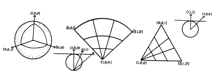
Figure 1: An octant of a sphere and two flat maps: To the left we see the positive octant of the sphere. In the middle there is a stereographic map of the octant centered at $(n_{0},n_{1},n_{2})=(1,0,0)$. On the right there is a gnomonic map centered at $\frac{1}{\sqrt{3}}(1,1,1)$. The projections are done respectively from the South Pole and from the center of the sphere, as shown. On each map four geodesics are drawn. A pair of these geodesics that meet an edge divides that edge into three equal parts. This gives an idea about how distances are distorted by the maps.

This takes care of the octant (the ”manifold with corners” in the language of toric geometry [2]). It becomes a picture of ${\bf CP}^{2}$ when we remember that each point in the interior really represents a flat torus, conveniently regarded as a parallelogram with opposite sides identified. The shape of the parallelogram is relevant. According to eq. (S0.Ex2) the lengths of the sides are

$$L_{1}=\int_{0}^{2{\pi}}ds=2{\pi}n_{1}\sqrt{1-n_{1}^{2}}\hskip 14.22636pt\mbox{and}\hskip 14.22636ptL_{2}=2{\pi}n_{2}\sqrt{1-n_{2}^{2}}\ .$$ (11)

The angle between them is given by

$$\cos{{\theta}_{12}}=-\frac{n_{1}n_{2}}{\sqrt{1-n_{1}^{2}}\sqrt{1-n_{2}^{2}}}\ .$$ (12)

The point is that the shape depends on where we are on the octant. So does the total area of the torus,

$$A=L_{1}L_{2}\sin{{\theta}_{12}}=4{\pi}^{2}n_{0}n_{1}n_{2}\ .$$ (13)

The ”biggest” torus occurs at the center of the octant. At the boundaries the area of the tori is zero. This is because there the tori degenerate to circles. Figure 2 shows how this happens. In effect an edge of the octant is a one parameter family of circles, in other words it is a ${\bf CP}^{1}$.

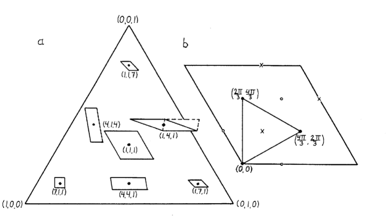
Figure 2: The octant really parametrizes a family of flat tori of varying sizes and shapes. In a) we indicate how the torus lying over each interior point changes with position in the octant. The position in the octant is given by an unnormalized vector. At the edges the tori degenerate to circles so that the edges are complex projective lines, while the corners of the octant represent points. Sometimes it is convenient to perform a little cutting and gluing of the parallelogram before thinking about the shape of the torus it defines, as indicated with dashed lines for the torus lying over the point $(1,4,1)$. The size of the octant relative to that of the tori is exaggerated in the picture. To bring this home we show, in b), the largest torus—the one sitting over $(1,1,1)$—decorated with three times three points corresponding to three mutually unbiased bases (represented respectively by crosses and filled and unfilled dots). They are all mutually unbiased with respect to the basis that forms the corners of the octant. The coordinates $({\nu}_{1},{\nu}_{2})$ are given for one basis.

It is crucial to realize that there is nothing special going on at the edges and corners of the octant, whatever the impression left by the map may be. Like the sphere, ${\bf CP}^{n}$ is a homogeneous space and looks the same from every point. To see this, note that any choice of an orthogonal basis in a 3 dimensional Hilbert space gives rise to 3 points separated by the distance ${\pi}/2$ from each other in ${\bf CP}^{2}$. In projective geometry the triplet of points arising from an orthogonal basis in the underlying vector space is known as a triangle of reference. By an appropriate choice of coordinates we can make any such triple of points sit at the corners of an octant in a picture identical to the one above.

To get used to the picture let us consider some submanifolds. ${\bf CP}^{2}$ is also known as the ”complex projective plane”. Every pair of points in this ”plane” defines a unique ”complex projective line” containing the pair of points, and such a ”line” is a ${\bf CP}^{1}$. Conversely a pair of complex projective lines always intersect at a unique point. Since a ${\bf CP}^{1}$ is always a sphere (of radius 1/2) the terminology may boggle some minds, but these intersection properties are precisely what defines a line in projective geometry. Through every point there passes a 2-sphere’s worth of complex projective lines, conveniently parametrized by the way they intersect the ”line at infinity”, that is the set of points at maximal distance from the given point, which in itself is a ${\bf CP}^{1}$. This is easily illustrated provided we arrange the picture so that the given point sits in a corner.

Another submanifold is the real projective plane ${\bf RP}^{2}$. It is defined in a way analogous to the definition of ${\bf CP}^{2}$ except that real rather than complex numbers are used. The points of ${\bf RP}^{2}$ are therefore in one-to-one correspondence with the set of lines through the origin in a three dimensional real vector space and also with the points of ${\bf S}^{2}/{\bf Z}^{2}$, that is to say the sphere with antipodal points identified. In its turn this is a hemisphere with antipodal points on the equator identified. ${\bf RP}^{2}$ is clearly a subset of ${\bf CP}^{2}$. It is illuminating to see how the octant picture is obtained, starting from the stereographic projection of a hemisphere (a unit disk) and folding it twice, as in Figure 3.

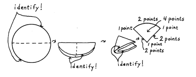
Figure 3: Using stereographic rather than gnomonic coordinates we show how the octant picture of the real submanifold ${\bf RP}^{2}$ is related to the standard description as a hemisphere with antipodal points on the equator identified.

Brody and Hughston [6] give a beautiful account of how the physics of a spin 1 particle is tied to the geometry of ${\bf CP}^{2}$. The space of all possible spin up states (with respect to some direction) forms a sphere of radius $1/\sqrt{2}$. This is not a complex projective line because of its size. The space of all possible spin 0 states (with respect to some direction) forms a sphere with antipodal points identified since such states do not distinguish up and down, hence this is an ${\bf RP}^{2}$. This is illustrated in Figure 4 under the assumption that the corners of the octant correspond to eigenstates of the operator $S_{z}$. It is interesting to observe that if we start from a ${\bf CP}^{1}$ (and place it as an edge in the picture) then we can increase the size of the sphere by deforming the edge, but we cannot shrink it. Therefore ${\bf CP}^{2}$ contains non-contractible 2-spheres, just as a torus contains non-contractible circles. Note that two non-contractible 2-spheres always touch at a point, essentially because two complex projective lines intersect in a unique point.

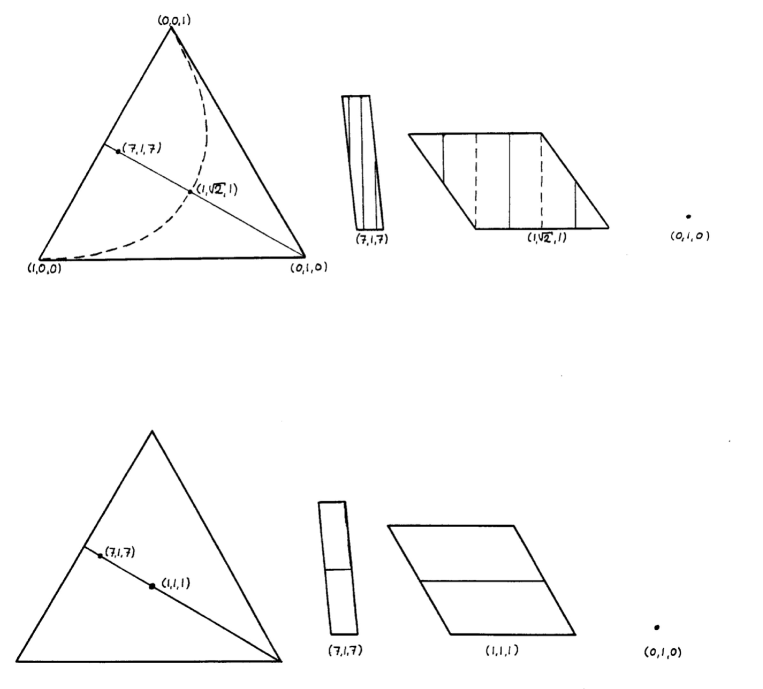
Figure 4: The physics of spin systems (above). The dashed curve represents a sphere with radius $1/\sqrt{2}$, and the solid line an ${\bf RP}^{2}$. Both are one parameter families of circles with points at one end. The sphere has a point at both ends, while for the real projective plane the circle sits in the torus in such a way that when the torus is squashed to a circle then the circle wrapped inside it suddenly collapses to a circle of half the size it had just before. We show how this happens by drawing two of the tori explicitly; again points on the sphere are represented by dashed lines and points on the ${\bf RP}^{2}$ by solid lines. For comparison we also show a complex projective line (below). This is a one parameter family of circles with points at both ends, as shown in the tori on the right hand side. Note also that any edge of the octant is a ${\bf CP}^{1}$, namely the ”line at infinity” with respect to the point in the opposite corner.

Next choose a point. Place it at a corner of the octant and surround it with a 3-sphere consisting of points at constant distance from the given point. In the picture this will appear as a curve in the octant with an entire torus sitting over each interior point of the curve. Readers familiar with the Hopf fibration know that ${\bf S}^{3}$ can be thought of as a one parameter family of tori with circles at the ends. The 3-sphere is round if the tori have a suitable rectangular shape. As we let the 3-sphere in Figure 5 grow the tori get more and more ”squashed” by the curvature of ${\bf CP}^{2}$, and the roundness gradually disappears. When the radius reaches its maximum value of ${\pi}/2$ the 3-sphere collapses to a 2-sphere, namely to the projective line ”at infinity”. Readers unfamiliar with the Hopf fibration may wish to consult Urbantke [1] at this point; let us just remark that only odd dimensional spheres can be squashed in this specific way (so it is no use to try to picture this in terms of the 2-sphere).

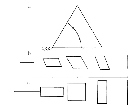
Figure 5: The set of points at constant distance from a corner form a squashed 3-sphere. In a) we show how such a submanifold appears in the octant. All the points in the torus lying over a point on the curve are included. In b) we show how the size and shape of the torus change as we move along the curve in the octant; at the ends of the interval the tori collapse to circles. For comparison, in c) we show the corresponding picture for a round 3-sphere.

Finally, a warning: The picture distorts distances in many ways. For instance, the distance between two points in a given torus is shorter than it looks, because the shortest path between them is not the same as a straight line within the torus itself. Technically, the flat tori are not totally geodesic. Note also that we have chosen to exaggerate the size of the octant relative to that of the tori in the pictures. To realize how much room there is in the largest torus, consider mutually unbiased measurements [7]. It is known that one can find 4 sets of orthonormal bases in the Hilbert space of a spin 1 particle such that the absolute value of the scalar product between members of different basises is $1/\sqrt{3}$ —clearly a kind of sphere packing problem if translated into geometrical terms by means of eq. (5). If one basis is represented by the corners of the octant, the remaining 3 times 3 basis vectors are situated in the torus over the center of the octant. (See figure 2.)

3. Separable and maximally entangled states in ${\bf CP}^{3}$.

We now wish to illustrate entanglement. This forces us to increase the dimension, since our system should be composed of two subsystems. If we choose to study pairs of entangled qubits the complex Hilbert space is ${\bf C}^{2}\otimes{\bf C}^{2}={\bf C}^{4}$, and the space of pure states becomes the six real dimensional space ${\bf CP}^{3}$. This is complex projective space. A preliminary remark about it is that it contains complex projective planes and lines (${\bf CP}^{2}$ and ${\bf CP}^{1}$) as submanifolds, and the intersection properties of these are just those of planes and lines in ordinary Euclidean space, with the important simplification that all troublesome exceptional cases (such as parallel planes that do not intersect in a line) are absent.

It is easy to make a picture of this six dimensional space. Choose the coordinates

$$(Z^{0},Z^{1},Z^{2},Z^{3})=(n_{0},n_{1}e^{i{\nu}_{1}},n_{2}e^{i{\nu}_{2}},n_{3}e^{i{\nu}_{3}})\ .$$ (14)

The phases now form a 3-torus (that we can picture as a rhomboid), while the non-negative real numbers $n_{0}$ etc. obey

$$n^{2}_{0}+n_{1}^{2}+n_{2}^{2}+n_{3}^{2}=1\ .$$ (15)

Hence they form a hyperoctant of the 3-sphere. Without further ado it is clear that if we perform a gnomonic projection centered at

$$(n_{0},n_{1},n_{2},n_{3})=\frac{1}{2}(1,1,1,1)$$ (16)

then we obtain a picture of this hyperoctant as a regular tetrahedron. In this picture straight lines correspond to geodesics on the round hyperoctant. Over each point in the interior there is a flat 3-torus of a definite shape. The faces of the tetrahedron are complex projective planes, its edges are complex projective lines, and its corners are points. Such pictures will appear soon.

We do not give the transformation to gnomonic coordinates here. This is because their only advantage is to give a nice symmetrical picture that is easy to draw, and most of our pictures can be drawn using only the fact that geodesics are straight lines, plus explicit knowledge of the two dimensional case. (Calculations should be performed in coordinate systems suited to calculation—for most purposes the embedding coordinates $n_{0}$, $n_{1}$, $n_{2}$, $n_{3}$ will do.)

Now, what about entanglement? Our illustrations in this section will depict submanifolds of states of constant entanglement, namely separable states (that are not entangled) and maximally entangled states. In the next section we show how states of ”intermediate entanglement” sit in ${\bf CP}^{3}$. The same story has been told before [8] but not in quite this way.

A brief review of the facts seems appropriate. State vectors for composite systems are conveniently written as

$$|{\Psi}\rangle=\frac{1}{\sqrt{N}}\sum_{i=0}^{n}\sum_{j=0}^{n}C_{ij}|i\rangle|j\rangle\ ,$$ (17)

where $C_{ij}$ is an $N\times N$ matrix with complex entries and during the review we keep the state vector normalized. Throughout the discussion we rely on a fixed way of splitting the Hilbert space into a tensor product of two smaller Hilbert spaces. In other words it has been agreed that the Hilbert space is ${\cal H}_{A}\otimes{\cal H}_{B}$ in a specific way. Otherwise the term ”entanglement” has no meaning. For the $2\times 2$ case let us agree that

$$(Z^{0},Z^{1},Z^{2},Z^{3})\equiv(C_{00},C_{01},C_{10},C_{11})\ .$$ (18)

The density matrix for the system can be written with composite indices, in the form

$${\rho}_{ij,kl}=\frac{1}{N}C_{ij}C^{*}_{kl}\ .$$ (19)

It has rank one because the system is in a pure state. Now suppose that we are performing experiments on one of the subsystems only. Then the relevant density matrix is the partially traced density matrix ${\rho}_{A}=\mbox{Tr}_{B}{\rho}$,

$${\rho}^{A}_{ik}=\sum_{j=0}^{n}{\rho}_{ij,kj}\ .$$ (20)

The rank of this matrix may well be greater than one. There are two extreme cases. The global state of the system may be a product state,

$$|{\Psi}\rangle=|A\rangle|B\rangle=\sum_{i=0}^{n}\sum_{j=0}^{n}(a_{i}|i\rangle)(b_{j}|j\rangle)\hskip 14.22636pt\Leftrightarrow\hskip 14.22636ptC_{ij}=a_{i}b_{j}\ ,$$ (21)

so the matrix $C$ is an outer (dyadic) product of two vectors $a$ and $b$. In this case the partially traced density matrix and the matrix $C_{ij}$ both have rank one and the individual subsystems are in pure states of their own. A global state of this kind is said to be un-entangled or separable. At the opposite end of the spectrum it happens that

$${\rho}^{A}_{ik}=\frac{1}{N}{\bf 1}\hskip 14.22636pt\Leftrightarrow\hskip 14.22636pt\sum_{j=0}^{n}C_{ij}C^{*}_{kj}={\delta}_{ik}\ .$$ (22)

This means that we know nothing at all about the state of the subsystems, even though the global state is precisely known. A global state of this kind is said to be maximally entangled. In between these cases are cases where the von Neumann entropy of ${\rho}^{A}$ takes some intermediate value. They are also entangled. It is known [9] that an arbitrary state in the Hilbert space ${\cal H}^{N}\otimes{\cal H}^{N}$ can be brought to the form

$$|{\Psi}\rangle=\sum_{i=0}^{n}c_{i}|i\rangle|i\rangle$$ (23)

by means of unitary transformations belonging to the subgroup $U(N)\times U(N)$, that is by ”local unitary” transformations acting independently on the two subsystems. The coefficients are square roots of the eigenvalues of the density matrix obtained when one subsystem is traced out, and hence they obey

$$\sum_{i=0}^{n}c_{i}^{2}=1\ .$$ (24)

This is known as the Schmidt decomposition and is explained in many places [10][11]. Once the Schmidt coefficients $c_{i}$ have been ordered (say by their sizes) they cannot be changed by local unitaries, so that they can be used to label the orbits of $U(N)\times U(N)$ in ${\bf CP}^{3}$. This ends our brief review of entanglement.

Now we are going to take a look (literally!) on the submanifolds that we mentioned. Consider first the separable states, as described in eq. (21). If we keep $|A\rangle$ fixed and vary $|B\rangle$ we sweep out a ${\bf CP}^{n}$ that lies, in its entirety, in the submanifold. Reversing the roles of $|A\rangle$ and $|B\rangle$ we sweep out another ${\bf CP}^{n}$, and every state in the submanifold can be reached by a combination of these operations. This means that the submanifold of separable states is the Cartesian product ${\bf CP}^{n}\times{\bf CP}^{n}$. For $N=2$ (that is $n=1$) we get the four real dimensional submanifold ${\bf CP}^{1}\times{\bf CP}^{1}$ sitting inside ${\bf CP}^{3}$, and the question is what it looks like in our picture. We want it to appear as a surface in the 3-torus, sitting over a surface in the octant. It is not a priori clear that this can be arranged. It depends on the arrangement of the octant picture. As a matter of fact it works nicely if the corners of the octant are made to represent separable states (and it does not work nicely if the corners represent the Bell basis). Explicitly, the state is separable if the rank of $C_{ij}$ is unity. Using the homogeneous coordinates introduced already in eq. (18) this means that

$$Z^{0}Z^{3}-Z^{1}Z^{2}=0\ .$$ (25)

In our coordinates this corresponds to the two real equations

$$n_{0}n_{3}-n_{1}n_{2}=0$$ (26)

$${\nu}_{1}+{\nu}_{2}-{\nu}_{3}=0\ .$$ (27)

The equation does separate into two equations, one independent of the phases and the other involving only them. This is a picture that can be drawn.

The surface in the 3-torus is, in itself, a flat 2-torus. The surface in the octant is easy to draw too because it has an interesting structure. In eq. (21), keep the state of the second subsystem fixed. Say $b_{0}/b_{1}=ke^{i{\phi}}$, where $k$ is a real number. This implies that

$$\frac{Z^{0}}{Z^{1}}=\frac{b_{0}}{b_{1}}\hskip 14.22636pt\Rightarrow\hskip 14.22636ptn_{0}=kn_{1}$$ (28)

$$\frac{Z^{2}}{Z^{3}}=\frac{b_{0}}{b_{1}}\hskip 14.22636pt\Rightarrow\hskip 14.22636ptn_{2}=kn_{3}\ .$$ (29)

As we vary the state of the first subsystem we sweep out a curve in the octant that is in fact a geodesic (the intersection between the 3-sphere and two hyperplanes through the origin in the embedding space). In our picture this is a straight line. In this way we see that the surface in the picture is a ruled surface swept out by two families of straight lines. If the octant of the 3-sphere (that is the interior of our gnomonic tetrahedron) had been flat this would have been an intrinsically curved surface, as a glance at Figure 6 shows. But the true intrinsic geometry of the surface we see in the picture is flat. To see this it is convenient to coordinatize the octant by means of Euler angles;

$$\left(\begin{array}[]{c}n_{0}\\ n_{1}\\ n_{2}\\ n_{3}\end{array}\right)=\left(\begin{array}[]{c}\sin{\frac{{\tau}-{\phi}}{2}}\sin{\frac{\theta}{2}}\\ \sin{\frac{{\tau}+{\phi}}{2}}\cos{\frac{\theta}{2}}\\ \cos{\frac{{\tau}-{\phi}}{2}}\sin{\frac{\theta}{2}}\\ \cos{\frac{{\tau}+{\phi}}{2}}\cos{\frac{\theta}{2}}\end{array}\right)\ .$$ (30)

A straightforward calculation now shows that the separability condition (26) is equivalent to ${\phi}=0$. The coordinate ${\tau}$ varies with the state of the first subsystem, and the coordinate ${\theta}$ with the other. The intrinsic metric of the surface that we see in the octant is

$$ds^{2}=\frac{1}{4}(d{\tau}^{2}+d{\theta}^{2})\ .$$ (31)

Hence it is an intrinsically flat surface embedded in a curved space; in the language of toric geometry the ”manifold with corners” of ${\bf CP}^{1}\times{\bf CP}^{1}$ is a flat square.

This little calculation has an interesting interpretation that we mention for the benefit of those readers who are familiar with the Hopf fibration of the 3-sphere [1]. The 3-sphere can be filled with a congruence of nowhere vanishing geodesics (”Villarceau circles”) that twist around each other but never meet. The Euler angles are adapted to this congruence in such a way that ${\tau}$ runs along the geodesics and the latter are labelled by ${\theta}$ and ${\phi}$. Thus we see that our surface is made up of a one parameter family of ”Hopf fibres”; actually there is another Hopf fibration with the opposite twist and this explains why the surface is ruled by two families of intersecting geodesics.

We are now ready to look at the space of separable states in ${\bf CP}^{3}$. It is given in Figure 6.

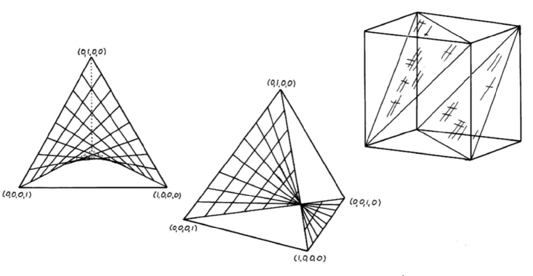
Figure 6: The separable states, or the submanifold ${\bf CP}^{1}\times{\bf CP}^{1}$ in ${\bf CP}^{3}$. It appears as a surface ruled by geodesics in the octant, and it must be remembered that there is a 2-torus sitting in the 3-torus over each of its interior points. The intrinsic geometry of the ”manifold with corners”, that is the ruled surface that we see in the octant, is actually flat. Two different perspectives of the octant are shown. The 3-torus is shown schematically as a cube.

We now turn to the maximally entangled states. According to eq. (22) a state is maximally entangled if and only if the matrix $C_{ij}$ is unitary. Since an overall factor of this matrix is irrelevant for the state we can use it to adjust the determinant of the matrix to equal one. The state now determines the matrix up to multiplication with an $N$th root of unity. We arrive at the conclusion that the space of maximally entangled states form the group manifold $SU(N)/{\bf Z}^{N}=U(N)/U(1)$ [12] [13]. The reason why this space turns up is that, like the separable states, the maximally entangled ones forms an orbit of the group of local unitary transformations. The group manifold $SU(N)/{\bf Z}^{N}$ and the product space ${\bf CP}^{n}\times{\bf CP}^{n}$ then spring to mind as the two most obvious candidates.

When $N=2$ we have $SU(2)/{\bf Z}^{2}=SO(3)$, and this happens to be the real projective space ${\bf RP}^{3}$. To see what it looks like in the picture we parametrize the unitary matrix $C_{ij}$ as

$$C_{ij}=\left(\begin{array}[]{cc}{\alpha}&{\beta}\\ -{\beta}^{*}&{\alpha}^{*}\end{array}\right)\hskip 14.22636pt\Rightarrow\hskip 14.22636ptZ^{\alpha}=({\alpha},{\beta},-{\beta}^{*},{\alpha}^{*})\ .$$ (32)

In our coordinates this yields three real equations, namely

$$n_{0}=n_{3}\hskip 34.1433ptn_{1}=n_{2}$$ (33)

$${\nu}_{1}+{\nu}_{2}-{\nu}_{3}={\pi}\ .$$ (34)

In the octant this is a single geodesic connecting the entangled edges and passing through the center of the tetrahedron. In the 3-torus it is a surface representing a flat 2-torus. So it appears as a one parameter family of 2-tori, in fact an ${\bf RP}^{3}$, as it should. Note that the geodesic in the octant crosses the separable surface where the 3-torus achieves its maximum size; this is how it manages to keep its distance from the entangled states (namely, every maximally entangled state is at the distance ${\pi}/4$ from the separable surface). This is shown in Figure 7, where we also show the location of the maximally entangled Bell basis

$$|{\psi}^{\pm}\rangle=|0\rangle|1\rangle\pm|1\rangle|0\rangle\hskip 22.76219pt|{\phi}^{\pm}\rangle=|0\rangle|0\rangle\pm|1\rangle|1\rangle\ .$$ (35)

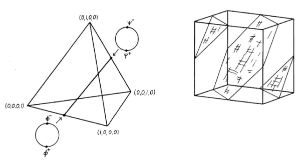
Figure 7: The maximally entangled states form an ${\bf RP}^{3}$’s worth of points, all at distance ${\pi}/4$ from the closest separable states. In the octant we see a single straight line; the location of the standard Bell basis is also shown. There is a 2-torus in the 3-torus (again shown schematically as a cube) over each interior point.

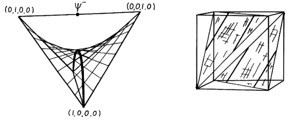
Figure 8: If the global system is in the Bell state $|{\Psi}^{-}\rangle$ and if we perform a complete measurement on one of the subsystems we end up on a sphere that lies on the separable surface. It is a one parameter family of circles as it should be. We show one such circle lying on the separable surface in the 3-torus on the right hand side.

Finally, let us illustrate the collapse of the wave function. If we perform a measurement on one of the subsystems the state of the composite system will ”jump” in the general direction of the separable surface. If the measurement is a von Neumann measurement we end up on the surface of separable states. The question is, where? The most likely possibility is on that point on the separable surface that is closest to the state we started out from. In the generic case this point is unique. (To compute it, first use local unitaries to bring the given state to the Schmidt form. Unitary transformations are isometries and do not change distances. It is now easy to see that the closest separable state is in fact the nearest corner of the Schmidt simplex. Generically this is unique.) Maximally entangled states are exceptional in that there is an entire 2-sphere’s worth of points on the separable surface at equal distance from the given state. This 2-sphere is not a complex projective line because its radius is $1/\sqrt{2}$ whereas a complex projective line is a sphere with radius $1/2$. We are equally likely to land anywhere on this 2-sphere. This is basically the statement that if the global state is completely entangled then we do not know anything about the state of a subsystem. So Figure 8 picture depicts that 2-sphere of separable states that is closest (at distance ${\pi}/4$) to the Bell state $|{\Psi}^{-}\rangle$. It consists of all states of the form $|+\rangle_{n}|-\rangle_{n}$ for some choice of direction ${\bf n}$.

4. Submanifolds of fixed entanglement.

We can go on to ask about states with some intermediate degree of entanglement. In the particular case when $N=2$ the remainder of ${\bf CP}^{N^{2}-1}$ is foliated by a one-parameter family of five dimensional orbits of local unitaries. We will not draw such a submanifold here but it can actually be done, and the result is much nicer than one might have thought. A pure state of intermediate entanglement has the Schmidt decomposition

$$|{\Psi}\rangle=\cos{\sigma}|++\rangle+\sin{\sigma}|--\rangle\ ,\hskip 22.76219pt0<{\sigma}<{\pi}/4\ .$$ (36)

The entanglement grows monotonically with the Schmidt angle ${\sigma}$. The partially traced density matrix (that arises when we trace over one of the subsystems) then has two unequal and non-zero eigenvalues ${\lambda}_{1}=\cos^{2}{\sigma}$ and ${\lambda}_{2}=\sin^{2}{\sigma}$. A minor calculation verifies that the partially traced density matrix has these eigenvalues if and only if

$$\cos{({\nu}_{3}-{\nu}_{1}-{\nu}_{2})}=\frac{n_{0}^{2}n_{3}^{2}+n_{1}^{2}n_{2}^{2}-\cos^{2}{\sigma}\sin^{2}{\sigma}}{2n_{0}n_{1}n_{2}n_{3}}\ .$$ (37)

When this equation has any solutions at all, it describes a 2-torus in the 3-torus, but this time its position within the 3-torus depends on where we are in the octant. There are three dimensions left to account for, and the pleasant surprise is that this appears as a volume that only partly fills the octant. Its boundaries are obtained by setting the right hand side of the preceding equation equal to $\pm 1$, that is by

$$(n_{0}n_{3}-n_{1}n_{2})^{2}\leq\cos^{2}{\sigma}\sin^{2}{\sigma}\leq(n_{0}n_{3}+n_{1}n_{2})^{2}\ .$$ (38)

When ${\sigma}$ is small it lies close to the separable surface, while for ${\sigma}$ close to ${\pi}/4$ what we see in the octant is a kind of three dimensional tube surrounding the maximally entangled line. We leave its precise appearance as an exercise for the reader. Note that the case $N=2$ is exceptional; when $N>2$ the orbits of local unitary transformations have codimension larger than one, there is no obviously canonical measure of pure state entanglement, and a much more intricate picture emerges. For illustrations of the $N=3$ case consult [14].

The situation is qualitatively similar to that of the orbits of $SU(2)$ in ${\bf CP}^{2}$ [4], also in the sense that the octant picture of the orbit looks nice but is poorly suited to do calculations. Once it is understood what a $U(2)\times U(2)$ orbit looks like we can watch it grow and shrink as we increase the entanglement. But to understand its intrinsic geometry it is better to proceed as follows: Choose a point in the orbit given in Schmidt form by

$$C^{S}_{ij}=\left(\begin{array}[]{cc}\cos{\sigma}&0\\ 0&\sin{\sigma}\end{array}\right)\ ,$$ (39)

where $C_{ij}$ is the matrix introduced in eq. (17) and ${\sigma}$ runs from $0$ to ${\pi}/4$; ${\sigma}$ is the Schmidt angle and increases monotonically with the entanglement. An arbitrary point in the orbit can be reached from the given one by means of unitary transformations of the factor Hilbert spaces. Actually $SU(2)$ transformations are enough, and these can be parametrized with Euler angles. That is to say that an arbitary point in the orbit can be given by a matrix $C_{ij}$ defined by

$$C=e^{-i{\phi}_{1}L_{z}}e^{i{\theta}_{1}L_{y}}e^{-i{\tau}_{1}L_{z}}C^{S}e^{-i{\tau}_{2}L_{z}}e^{-i{\theta}_{2}L_{y}}e^{-i{\phi}_{2}L_{z}}$$ (40)

where $L_{y}$ and $L_{z}$ are the angular momentum operators in the standard representation (and one of the group elements appears transposed in the formula). In the calculation one sees that only ${\tau}\equiv{\tau}_{1}+{\tau}_{2}$ matters. After a still fairly elaborate calculation we obtain the Fubini-Study metric in the form

$$ds^{2}=d{\sigma}^{2}+dl^{2}\ ,$$ (41)

where $dl^{2}$ is the intrinsic metric on the five dimensional orbit labelled by $0<{\sigma}<{\pi}/4$. Explicitly

$$dl^{2}=\frac{1}{4}(d{\theta}^{2}_{1}+\sin^{2}{{\theta}_{1}}d{\phi}_{1}^{2}+d{\theta}^{2}_{2}+\sin^{2}{{\theta}_{2}}d{\phi}_{2}^{2}+$$

$$+2\sin{2{\sigma}}(\cos{\tau}\sin{{\theta}_{1}}\sin{{\theta}_{2}}d{\phi}_{1}d{\phi}_{2}-d{\theta}_{1}d{\theta}_{2}-$$

(42)

$$-\sin{\tau}\sin{{\theta}_{2}}d{\theta}_{1}d{\phi}_{2}-\sin{\tau}\sin{{\theta}_{1}}d{\theta}_{2}d{\phi}_{1})$$

$$+\sin^{2}{2{\sigma}}(d{\tau}+\cos{{\theta}_{1}}d{\phi}_{1}+\cos{{\theta}_{2}}d{\phi}_{2})^{2})$$

where $0<{\phi}_{1},{\phi}_{2},{\tau}<2{\pi}$, $0<{\theta}_{1},{\theta}_{2}<{\pi}$. When ${\sigma}=0$ this reduces to the metric of ${\bf S}^{2}\times{\bf S}^{2}$ as it should, while the coordinates misbehave when ${\sigma}={\pi}/4$. The square root of the determinant of this metric is

$$\sqrt{g}=\frac{1}{2^{5}}\cos^{2}{2{\sigma}}\sin{2{\sigma}}\sin{{\theta}_{1}}\sin{{\theta}_{2}}\ .$$ (43)

(Actually the clever way to compute this is to go via the symplectic form presented in section 6. The coordinates used here are well adapted for this task.) The volume of a given orbit can now be computed and is found to be

$$\mbox{vol}({\sigma})={\pi}^{3}\cos^{2}{2{\sigma}}\sin{2{\sigma}}\ .$$ (44)

Dividing by the volume ${\pi}^{3}/6$ of ${\bf CP}^{3}$ we obtain a probability distribution $P({\sigma})$ for the Schmidt angle ${\sigma}$. Note that the unitarily invariant distribution over the set of pure states used here induces the unitary distribution inside the Bloch ball for the mixed states ${\rho}_{A}=\mbox{Tr}_{B}|{\psi}\rangle\langle{\psi}|$. [15].

Another coordinatization of the orbit works better when the entanglement is close to maximal. Above we used two arbitrary unitary matrices $u_{1}$ and $u_{2}$ to write

$$C=u_{1}C^{S}u_{2}\ .$$ (45)

If we introduce $u_{3}=u_{1}u_{2}$ this becomes

$$C=u_{1}C^{S}u_{1}^{-1}u_{3}\ .$$ (46)

Now one Euler angle in $u_{1}$ is irrelevant; moreover we see directly that in the maximally entangled case—when $C^{S}$ becomes diagonal—the orbit collapses to the group manifold of $SU(2)/{\bf Z}^{2}={\bf RP}^{3}$. One can check that the embedding is isometric.

Since we have a foliation of ${\bf CP}^{3}$ with five dimensional hypersurfaces—except for the exceptional subsets where the entanglement either vanishes or is maximal—it is interesting to look at the second fundamental form of these hypersurfaces. One finds that the trace of the extrinsic curvature tensor is

$$K=\frac{4}{\cos{2{\sigma}}\sin{2{\sigma}}}(\cos^{2}{2{\sigma}}-2\sin^{2}{2{\sigma}})\ .$$ (47)

A foliation with the property that $K$ is constant on each hypersurface is called a constant mean curvature foliation. We observe that $K=0$ when $\tan{2{\sigma}}=1/\sqrt{2}$, that is when the volume of the orbit is maximal.

Let us emphasize again that this state of affairs is special to two qubit entanglement; in higher dimensions a much more intricate story emerges. See ref. [16] for the dimensions of the local orbits that appear in the $N\times N$ case.

5. An Aside on the Statistical Geometry of Simplices.

Due to obvious limitations we cannot literally draw our picture when the dimension of the Hilbert space exceeds four. There is one particular aspect of entanglement that we can draw up to dimension $4\times 4$, however. This is the Schmidt simplex, that is to say all states that have the form given in eq. (23). As we mentioned a central fact is that given any state there is a local unitary transformation that brings it into the Schmidt simplex. It is a simplex essentially because of eq. (24). It is clear that the Schmidt simplex is an $N-1$ dimensional (hyper-)face of the hyperoctant that forms a part of our picture. It is easy to check that its intrinsic geometry—induced by the Fubini-Study metric—is round, so in itself it forms the (hyper-)octant of a round sphere. Using gnomonic coordinates we draw it as a flat simplex.

The Schmidt simplex should not be confused with another simplex having the same pure states sitting in its corners, namely the statistical simplex whose points represent density matrices in the convex cover of these $N$ states. The latter is an $N-1$ dimensional subset of the $N^{2}-1$ dimensional space of density matrices, consisting of density matrices that can be simultaneously diagonalized. Usually the probabilities $p_{i}$ are used as barycentric coordinates on this simplex, which then consists of all density matrices of the form

$${\rho}=\sum_{i=0}^{n}p_{i}|i\rangle\langle i|\ ,\hskip 14.22636pt\sum_{i=0}^{n}p_{i}=1\ .$$ (48)

There is an obvious flat metric on this simplex that has the property that the density matrices obtained by taking the mixture of two density matrices in the set appears as a straight line connecting two extreme points representing the original pair of density matrices. There is also a round metric on this simplex that is induced by the Bures metric on the set of all density matrices [17]; it captures the statistical geometry of density matrices [18].

A possible confusion now arises because we have one round and two flat metrics on the same simplex, the latter two being the metric that makes statistical mixtures appear as straight lines and the metric that naturally exists on the gnomonic coordinate plane. These are not the same. If we draw the round simplex using gnomonic coordinates the statistical mixtures will be represented by curves, as in Figure 9. This must be kept in mind if we ask (say) how far away the corners are from the interior: The usual statement [5] that the corners are further away than they seem refers to the coordinates $p_{i}$; the significance of these coordinates is that they manifest the convexity properties of the simplex.

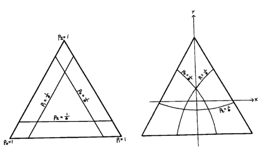
Figure 9: The statistical simplex of diagonal density matrices of size $N=3$, drawn with the eigenvalues $p_{i}$ as barycentric coordinates (left), and the same simplex drawn as a round simplex using gnomonic coordinates $x,y$ (right). Corners represent pure states while the centers of the triangles represent the maximally mixed state. The round (statistical) distance from a given point to the nearest corner appears too short in the former picture and too long in the latter.

Note also that we have two different round simplices with pure states in its corners, namely the Schmidt simplex that consists of pure states, and the statistical simplex that consists of density matrices.

6. An aside on symplectic geometry.

The manifold ${\bf CP}^{n}$ does not enjoy a metric geometry only. It also has a symplectic structure closely allied to it; in physicist’s language it is a phase space equipped with a Poisson bracket in a natural way. In more mathematical language there is a symplectic (closed, non-degenerate) 2-form around. Since we are praising the virtues of a special coordinate system here it seems natural to mention that the symplectic 2-form ${\Omega}$ also takes a simple form in this coordinate system. In effect

$${\Omega}=2i\frac{Z\cdot\bar{Z}dZ\cdot\wedge d\bar{Z}-\bar{Z}\cdot dZ\wedge d\bar{Z}\cdot Z}{Z\cdot\bar{Z}Z\cdot\bar{Z}}=\hskip 17.07164pt$$

(49)

$$\hskip 17.07164pt=4(n_{1}dn_{1}\wedge d{\nu}_{1}+n_{2}dn_{2}\wedge d{\nu}_{2}+n_{3}dn_{3}\wedge d{\nu}_{3})\ ,$$

where the last line is for $n=3$. Hence we can think of $n_{i}^{2}$ as being ”canonically conjugate” to the phase ${\nu}_{i}$; in effect these are action-angle variables. There is a nice interplay between the symplectic geometry and the geometry of entanglement. In particular a straightforward calculation verifies that the space of maximally entangled states is a Lagrangian submanifold. A submanifold of dimension $D$ in a symplectic space of dimension $2D$ is said to be Lagrangian if and only if the symplectic form induced on the submanifold by the embedding vanishes; mathematicians know that $SU(N)/{\bf Z}^{N}$ is a Lagrangian submanifold of ${\bf CP}^{N^{2}-1}$ but no complete classification of Lagrangian submanifolds is available [19].

Let us now specialize to ${\bf CP}^{3}$, and give the symplectic form in the coordinates introduced in eqs. (39)-(40):

$${\Omega}=2\sin{2{\sigma}}(d{\sigma}\wedge d{\tau}+\cos{{\theta}_{1}}d{\sigma}\wedge d{\phi}_{1}+\cos{{\theta}_{2}}d{\sigma}\wedge d{\phi}_{2})+$$

(50)

$$+\cos{2{\sigma}}(\sin{{\theta}_{1}}d{\theta}_{1}\wedge d{\phi}_{1}+\sin{{\theta}_{2}}d{\theta}_{2}\wedge d{\phi}_{2})\ .$$

On the five dimensional orbits of local unitaries the first line goes away since ${\sigma}$ is constant. The symplectic form is then degenerate and goes smoothly over to the symplectic form on ${\bf S}^{2}\times{\bf S}^{2}$ as ${\sigma}$ goes to zero. In the language often used by physicists interested in constrained systems [20] the equation (37) that defines the orbit is a first class constraint and the coordinate ${\tau}$ runs along the gauge orbits.

We observe that the volume element discussed in section 5 is easy to derive using

$$\sqrt{g}d^{6}x=\frac{1}{3!}(\frac{1}{4}{\Omega})\wedge(\frac{1}{4}{\Omega})\wedge(\frac{1}{4}{\Omega})\ .$$ (51)

This alternative way of computing the volume element is always open on Kähler manifolds such as ${\bf CP}^{n}$.

7. Envoi.

We hope that our results serve to bring home the fact that ${\bf CP}^{n}$ has an interesting geometry, that this geometry can be visualized without too much effort, and that the resulting picture has something to tell us about the physics of entanglement—at the very least, that it serves to illustrate it.

Acknowledgement:

We thank Torsten Ekedahl for some help.

References

- [1] H. Urbantke, Am. J. Phys. 59 (1991) 503.
- [2] G. Ewald: Combinatorial Convexity and Algebraic Geometry, Springer, New York 1996
- [3] Arvind, K. S. Mallesh and N. Mukunda, J. Phys. A30 (1997) 2417.
- [4] N. Barros e Sá, J. Phys. A34 (12001) 4831..
- [5] W. K. Wootters, Phys. Rev. D23 (1981) 357.
- [6] D. C. Brody and L. P. Hughston, J. Geom. Phys. 38 (2001) 19.
- [7] I. D. Ivanovic, J. Phys. A14 (1981) 3241.
- [8] M. Kuś and K. Życzkowski, Phys. Rev. A63 (2001) 03207-13.
- [9] H. Everett, Rev. Mod. Phys. 29 (1957) 454.
- [10] A. Peres: Quantum Theory: Concepts and Methods, Kluwer Academic, Dordrecht 1993.
- [11] A. Ekert and P. L. Knight, Am. J. Phys. 63 (1995) 415.
- [12] D. I. Fivel, The Lattice Dynamics of Completely Entangled States and Its Application to Communication Schemes, hep-th/9409148.
- [13] K. G. H. Vollbrecht and R. F. Werner, J. Math. Phys. 41 (2000) 6772.
- [14] K. Życzkowski and I. Bengtsson, Relativity of Pure States Entanglement, quant-ph/0103027.
- [15] K. Życzkowski and H.-J. Sommers, Induced measures in the space of mixed quantum states, quant-ph/0012101.
- [16] M. Sinolecka, K. Życzkowski and M. Kuś, to appear.
- [17] A. Uhlmann, Rep. Math. Phys. 33 (1993) 253.
- [18] S. L. Braunstein and C. M. Caves, Phys. Rev. Lett. 22 (1994) 3439.
- [19] R. Bryant, private communication.
- [20] A. Ashtekar and M. Stillerman, J. Math. Phys. 27 (1986) 1319.