Entanglement purification with noisy apparatus can be used to factor out an eavesdropper

Abstract

We give a proof that entanglement purification, even with noisy apparatus, is sufficient to disentangle an eavesdropper (Eve) from the communication channel. Our proof applies to all possible attacks (individual and coherent). Due to the quantum nature of the entanglement purification protocol, it is also possible to use the obtained quantum channel for secure transmission of quantum information.

I Introduction

Quantum communication exploits the quantum properties of its information carriers for communication purposes such as the distribution of secure cryptographic keys in quantum cryptography Bennett and Brassard (1985); Ekert (1991) and the communication between distant quantum computers in a network Cirac et al. (1997). A central problem of quantum communication is how to faithfully transmit unknown quantum states through a noisy quantum channel Schumacher (1996). While information is sent through such a channel (for example an optical fiber), the carriers of the information interact with the channel, which gives rise to the phenomenon of decoherence and absorbtion; an initially pure quantum state becomes a mixed state when it leaves the channel. For quantum communication purposes, it is however necessary that the transmitted qubits retain their genuine quantum properties, for example in form of an entanglement with qubits on the other side of the channel.

In quantum cryptography, noise in the communication channel plays a crucial role: In the worst-case scenario, all noise in the channel is attributed to an eavesdropper, who manipulates the qubits in order to gain as much information on their state as possible, while introducing only a moderate level of noise.

To deal with this situation, two different techniques have been developed: Classical privacy amplification allows the eavesdropper to have partial knowledge about the raw key built up between the communicating parties Alice and Bob. From the raw key, a shorter key is “distilled” about which Eve has vanishing (i. e. exponentially small in some chosen security parameter) knowledge. Despite of the simple idea, proofs taking into account all eavesdropping attacks allowed by the laws of quantum mechanics have shown to be technically involved Mayers (1996); Biham et al. (2000); Inamori . Recently, Shor and Preskill Shor and Preskill (2000) have given a simpler physical proof relating the ideas in Mayers (1996); Biham et al. (2000) to quantum error correcting codes Calderbank and Shor (1996) and, equivalently, to one-way entanglement purification protocols. Quantum privacy amplification (QPA) Deutsch et al. (1996), on the other hand, employs a two-way entanglement purification recurrence protocol Bennett et al. (1996a) that eliminates any entanglement with an eavesdropper by creating a few perfect EPR pairs out of many imperfect (or impure) EPR pairs. The perfect EPR pairs can then be used for secure key distribution in entanglement-based quantum cryptography Deutsch et al. (1996); Ekert (1991); Bennett et al. (1992). In principle, this method guarantees security against any eavesdropping attack. However, the problem is that the QPA protocol assumes ideal quantum operations. In reality, these operations are themselves subject to noise. As shown in Briegel et al. (1998); Dür et al. (1999); Giedke et al. (1999), there is an upper bound $F_{\text{max}}$ for the achievable fidelity of EPR pairs which can be distilled using noisy apparatus. A priori, there is no way to be sure that there is no residual entanglement with an eavesdropper. This problem could be solved if Alice and Bob had fault tolerant quantum computers at their disposal, which could then be used to reduce the noise of the apparatus to any desired level. This was an essential assumption in the security proof given by Lo and Chau Lo and Chau (1999).

In this paper, we show that the standard two-way entanglement purification protocols alone, which have been developed by Bennett at al. Bennett et al. (1996b, a) and later by Deutsch et al. Deutsch et al. (1996), with some minor modifications to accomodate certain security aspects as discussed below, can be used to efficiently establish a perfectly private quantum channel, even when both the physical channel connecting the parties and the local apparatus used by Alice and Bob are noisy.

In Section II we will briefly review the concepts of entanglement purification. Section III will give the main result of our work: we prove that it is possible to factor out an eavesdropper using EPP, even when the apparatus used by Alice and Bob is noisy. We conclude the paper with a discussion in Section IV.

II Entanglement purification

As two-way entanglement purification protocols (2–EPP) play an important role in this paper, we will briefly review one example of a a recurrence protocol which was described in Deutsch et al. (1996), and called quantum privacy amplification (QPA) by the authors. It is important to note that we distinguish the entanglement purification protocol from the distillation process: the first consists of probabilistic local operations (unitary rotations and measurements), where two pairs of qubits are combined, and either one or zero pairs are kept, depending on the measurement outcomes. The latter, on the other hand, is the procedure where the purification protocol is applied to large ensemble of pairs recursively (see Fig. (1)).

Figure 1: The entanglement purification protocol (a) and the entanglement distillation process (b).

In the quantum privacy amplification 2–EPP, two pairs of qubits, shared by Alice and Bob, are considered to be in the state $\rho_{A_{1}B_{1}}\otimes\rho_{A_{2}B_{2}}$. Without loss of generality (see later), we may assume that the state of the pairs is of the Bell-diagonal form,

$$\rho_{AB}=A\left|\Phi^{+}\right\rangle\!\left\langle\Phi^{+}\right|+B\left|\Psi^{-}\right\rangle\!\left\langle\Psi^{-}\right|+C\left|\Psi^{+}\right\rangle\!\left\langle\Psi^{+}\right|+D\left|\Phi^{-}\right\rangle\!\left\langle\Phi^{-}\right|.$$ (1)

Following Deutsch et al. (1996), the protocol consists of three steps:

1. Alice applies to her qubits a $\pi/2$ rotation, $U_{x}$, Bob a $-\pi/2$ rotation about the $x$ axis, $U_{x}^{-1}$.

2. Alice and Bob perform the bi-lateral CNOT operation

   $$\mathrm{BCNOT_{A_{1}B_{1}}^{A_{2}B_{2}}}=\mathrm{CNOT}_{A_{1}}^{A_{2}}\otimes\mathrm{CNOT}_{B_{1}}^{B_{2}}$$

   on the four qubits.

3. Alice and Bob measure both qubits of the target pair $A_{2}B_{2}$ of the BCNOT operation in the $z$ direction. If the measurement results coincide, the source pair $A_{1}B_{1}$ is kept, otherwise it is discarded. The target pair is always discarded, as it is projected onto a product state by the bilateal measurement.

By a straigtforward calculation, one gets the result that the state of the remaining pair is still a Bell diagonal state, with the diagonal coefficients Deutsch et al. (1996)

$$\begin{split}A^{\prime}&=\frac{A^{2}+B^{2}}{N},\quad B^{\prime}=\frac{2CD}{N}\\ C^{\prime}&=\frac{C^{2}+D^{2}}{N},\quad D^{\prime}=\frac{2AB}{N},\\ \end{split}$$ (2)

and the normalization coefficient $N=(A+B)^{2}+(C+D)^{2}$, which is the probability that Alice’s and Bob’s measurement results in step 3 coincide. Note that, up to the normalization, these recurrence relations are a quadratic form in the coefficients $A,B,C,$ and $D$. These relations allow for the following interpretation (which can be used to obtain the relations (2) in the first place): As all pairs are in the Bell diagonal state (1), one can interpret $A,B,C,$ and $D$ as the relative frequencies in the ensemble of all pairs of the states $\left|\Phi^{+}\right\rangle,\left|\Psi^{-}\right\rangle,\left|\Psi^{+}\right\rangle,$ and $\left|\Phi^{-}\right\rangle$, respectively. By looking at (2) one finds that the result of combining two $\left|\Phi^{+}\right\rangle$ or two $\left|\Psi^{-}\right\rangle$ pairs is a $\left|\Phi^{+}\right\rangle$ pair, combining a $\left|\Psi^{+}\right\rangle$ and a $\left|\Phi^{-}\right\rangle$ (or vice versa) yields a $\left|\Psi^{-}\right\rangle$ pair, and so on. Combinations of $A,B,C,$ and $D$ that do not occur in (2), namely $AC$, $AD$, $BC$ and $BD$, are “filtered out”, i. e. they give different measurement results for the bilateral measurement in step 3 of the protocol. We will use this way of calculating recurrence relations for more complicated situations later.

Numerical calculations Deutsch et al. (1996) and, later, an analytical investigation Macchiavello (1998) have shown that for all initial states (1) with $A>1/2$, the recurrence relations (2) approach the fixpoint $A=1,B=C=D=0$; this means that given a sufficiently large number of initial pairs, Alice and Bob can distill asymptotically pure EPR pairs.

III Factorization of Eve

In the previous section it has been assumed that Alice and Bob have perfect apparatus at their disposal, which they use to execute the protocol. For the following security analysis, we shall consider a more general scenario where this assumption is abandoned. As mentioned in the introduction, there is an upper bound $F_{\mathrm{max}}$ for the attainable fidelity of the distilled pairs, when the apparatus used by Alice and Bob is noisy Briegel et al. (1998); Dür et al. (1999). For quantum cryptography the question arises: can these imperfect pairs still be used for secure key distribution?

In this section we will show that 2–EPP with noisy apparatus is sufficient to factor out Eve in the Hilbertspace of Alice, Bob, their labs and Eve. For the proof, we will first introduce the concept of the lab demon as a simple model of noise. Then we will consider the special case of binary pairs, where we have obtained analytical results. Using the same techniques, we generalize the result to the case of Bell diagonal ensembles. The most general case of correlated non Bell-diagonal can be reduced to the case of Bell diagonal states Aschauer and Briegel .

III.1 The effect of noise

In this section we will answer the following question: what is the effect of an error, introduced by some noisy operation at a given point of the distillation process? To keep the argument transparent, we restrict our attention to the following type of noise:

• It acts locally, i. e. noise does not introduce correlations between remote quantum systems.

• Noise is memoryless, i. e. on a timescale imposed by the sequence of steps in a given protocol, there are no correlations between the “errors” that occur at different times.

The action of noisy apparatus on a quantum system in state $\rho\in\mathcal{B}(\mathcal{H})$ can be formally described by some trace conserving, completely positive map. Any such map can be written in the operator-sum representation Kraus (1983); Schumacher (1996),

$$\rho\rightarrow\sum_{i}A_{i}\rho A_{i}^{\dagger},$$ (3)

with linear operators $A_{i}$, that fulfill the normalization condition $\sum_{i}AA^{\dagger}=\mathbf{1}$. The operators $A_{i}$ are the so-called Kraus operators Kraus (1983).

As we have seen above, in the purification protocol the CNOT operation, which acts on two qubits $a$ and $b$, plays an important role. For that reason, it is necessary to consider noise which acts on a two-qubit Hilbert space $\mathcal{H}=\mathbb{C}^{2}_{a}\otimes\mathbb{C}^{2}_{b}$. Eq. (3) describes the most general non-selective operation that can, in principle, be implemented. For technical reasons, however, we restrict our attention to the case that the Kraus operators are proportional to products of Pauli matrices. The reason for this choice is that Pauli operators map Bell states onto Bell states, which will allow us to introduce the very useful concept of error flags later. Eq. (3) can then be written as

$$\rho_{ab}\rightarrow\sum_{\mu,\nu=0}^{3}f_{\mu\nu}\sigma_{\mu}^{(a)}\sigma_{\nu}^{(b)}\rho_{ab}\sigma_{\mu}^{(a)}\sigma_{\nu}^{(b)}\,,$$ (4)

with the normalization condition $\sum_{\mu,\nu=0}^{3}f_{\mu\nu}=1$. Note that Eq. (4) includes, for an appropriate choice of the coefficients $f_{\mu\nu}$, the one- and two-qubit depolarizing channel and combinations thereof, as studied in Briegel et al. (1998); Dür et al. (1999); but it is more general. Below, we will refer to these special Kraus operators as error operators.

The coefficients $f_{\mu\nu}$ can be interpreted as the joint probability that the Pauli rotations $\sigma_{\mu}$ and $\sigma_{\nu}$ occur on qubits $a$ and $b$, respectively. For pedagogic purposes we employ the following interpretation of (4): Imagine that there is a (ficticious) little demon in Alice’s laboratory – the “lab demon” – which applies in each step of the distillation process randomly, according to the probability distribution $f_{\mu\nu}$, the Pauli rotation $\sigma_{\mu}$ and $\sigma_{\nu}$ to the qubits $a$ and $b$, respectively. The lab demon summarizes all relevant aspects of the lab degrees of freedom involved in the noise process.

Noise in Bob’s laboratory, can, as long as we restrict ourselves to Bell diagonal ensembles, be attributed to noise introduced by Alice’s lab demon, without loss of generality. It is also possible to think of a second lab demon in Bob’s lab who acts similarly to Alice’s lab demon. This would, however, not affect the arguments employed in this paper.

The lab demon does not only apply rotations randomly, he also maintains a list in which he keeps track of which rotation he has applied to which qubit pair in which step of the distillation process. What we will show in the following section is that, from the mere content of this list, the lab demon will be able to extract – in the asymptotic limit – full information about the state of each residual pair of the ensemble. This will then imply that, given the lab demons knowledge about the flags, the state of the distilled ensemble is a tensor product of pure Bell states. Eve cannot not have information on the specific sequence of Bell pairs (in addition to their relative frequencies) — otherwise she would also be able to learn, to some extent, at which stage the lab demon has applied which rotation.

From that it follows that Eve is factored out, i. e. Alice and Bob describe their pairs with the state

$$\rho_{\mathrm{ABEL}}=\left(\sum_{i,j=0}^{1}f^{(i,j)}_{\mathrm{L}}\left|\mathcal{B}_{i,j}\right\rangle_{\!\mathrm{AB}}\!\left\langle\mathcal{B}_{i,j}\right|\right)\otimes\rho_{\mathrm{E}}.$$ (5)

It remains to be shown that the same argument applies to a realistic scenario where the lab demon is replaced by some “real” noise source. To be specific, in the following argument we show that all quantum or classical devices that share the same noise characteristics are equally secure. First we note that a communication protocol is secure if and only if there exists no eavesdropping strategy; this fact can, in priciple, be determined by cooperating communication parties. On the other hand, all devices with identical noise caracteristics are quantum mechanically described by the same completely positive trace conserving map, so that a initial state $\rho_{i}$ is mapped onto a final state $\rho_{f}$, independend from the physical realization of the map. This means that there is no way do distinguish the devices by only looking at the input and output states. For the case of noisy apparatus that is used for entanglement purification we get thus the following result: a device the implements (4) with a lab demon cannot be distinguished from any device that introduces noise due to some “real” noise source; in particular, the devices must lead to the same level of security (regardless whether or not error flags are measured or calculated by anybody): otherwise they would be distinguishable.

In order to separate conceptual from technical considerations and to obtain analytical results, we will first concentrate on the special case of binary pairs and a simplified error model. After that, we generalize the results to ensembles which are diagonal in the Bell basis.

III.2 Binary pairs

In this section we restrict our attention to pairs in the state

$$\rho_{AB}=A\left|\Phi^{+}\right\rangle_{\!AB}\!\left\langle\Phi^{+}\right|+B\left|\Psi^{+}\right\rangle_{\!AB}\!\left\langle\Psi^{+}\right|,$$ (6)

and to errors of the form

$$\rho_{AB}^{(1)}\otimes\rho_{AB}^{(2)}\rightarrow\sum_{\mu,\nu\in\{0,1\}}f_{\mu\nu}U^{(1)}_{\mu}U^{(2)}_{\nu}\rho_{AB}^{(1)}\otimes\rho_{AB}^{(2)}{U^{(1)}_{\mu}}^{\dagger}{U^{(2)}_{\nu}}^{\dagger}$$ (7)

with $U_{0}^{(1,2)}=\text{id}^{(1,2)}$ and $U_{1}^{(1,2)}={\sigma_{x}}^{(1,2)}$. Eq. (7) describes a two-bit correlated spin-flip channel. The indices 1 and 2 indicate the source and target bit of the bilateral CNOT (BCNOT) operation, respectively. It is straightforward to show that, using this error model in the 2–EPP, binary pairs will be mapped onto binary pairs.

At the beginning of the distillation process, Alice and Bob share an ensemble of pairs described by (6). Let us imagine that the lab demon attaches one classical bit to each pair, which he will use for book-keeping purposes. At this stage, all of these bits, which we call “error flags”, are set to zero. This reflects the fact that the lab demon has the same a priori knowledge about the state of the ensemble as Alice and Bob.

In each purification step, two of the pairs are combined. The lab demon first simulates the noise channel (7) on each pair of pairs by the process described. Whenever he applies a $\sigma_{x}$ operation to a qubit, he inverts the error flag of the corresponding pair. Alice and Bob then apply the 2–EPP to each pair of pairs; if the measurement results in the last step of the protocol coincide, the source pair will be kept. Obviously, the error flag of that remaining pair will also depend on the error flag of the the target pair, i. e. the error flag of the remaining pair is a function of the error flags of both “parent” pairs, which we call the flag update function. Since for binary pairs the error flag consists of one bit, there are 16 different flag update functions in total. From these, the lab demon chooses the logical AND function as the flag update function, i. e. the error flag of the remaining pair is set to “1” if and only if both parent’s error flags had the value “1”.

After each purification step, the lab demon divides all pairs into two subensembles, according to the value of their error flags. By a straightforward calculation, one finds for the coefficients $A_{i}$ and $B_{i}$, which completely describe the state of the pairs in the subensemble $i$, the following recurrence relations:

$$\begin{split}A_{0}^{\prime}=&\frac{1}{N}(f_{00}(A_{0}^{2}+2A_{0}A_{1})+f_{11}(B_{1}^{2}+2B_{0}B_{1})\\ &+f_{s}(A_{0}B_{1}+A_{1}B_{1}+A_{0}B_{0}))\\ A_{1}^{\prime}=&\frac{1}{N}\left(f_{00}A_{1}^{2}+f_{11}B_{0}^{2}+f_{s}A_{1}B_{0}\right)\\ B_{0}^{\prime}=&\frac{1}{N}(f_{00}(B_{0}^{2}+2B_{0}B_{1})+f_{11}(A_{1}^{2}+2A_{0}A_{1})\\ &+f_{s}(B_{0}A_{1}+B_{1}A_{1}+B_{0}A_{0}))\\ B_{1}^{\prime}=&\frac{1}{N}\left(f_{00}B_{1}^{2}+f_{11}A_{0}^{2}+f_{s}B_{1}A_{0}\right)\end{split}$$ (8)

with $N=(f_{00}+f_{11})((A_{0}+A_{1})^{2}+(B_{0}+B_{1})^{2})+2f_{s}(A_{0}+A_{1})(B_{0}+B_{1})$ and $f_{s}=f_{01}+f_{10}$.

For the case of uncorrelated noise, $f_{\mu\nu}=f_{\mu}f_{\nu}$, we find an analytical expression for the relevant fixpoint of the map (8):

$$\begin{split}A_{0}^{\infty}&=\frac{4f_{0}^{2}-4f_{0}+(2f_{0}-1)\sqrt{4f_{0}-3}+1}{2(2f_{0}-1)^{2}},\\ A_{1}^{\infty}&=0,\quad B_{0}^{\infty}=0,\quad B_{1}^{\infty}=1-A_{0}^{\infty}.\end{split}$$ (9)

Note that, while Eq. (9) gives a fixpoint of (8) for $f_{0}\geq 3/4$, this does not imply that this fixpoint is an attractor. In order to investigate the attractor properties, we calculate the eigenvalues of the matrix of first derivatives,

$$M_{D}=\left.\left(\begin{array}[]{c c c}\frac{\partial A_{0}^{\prime}}{\partial A_{0}}&\cdots&\frac{\partial B_{1}^{\prime}}{\partial A_{0}}\\ \vdots&\ddots&\vdots\\ \frac{\partial A_{0}^{\prime}}{\partial B_{1}}&\cdots&\frac{\partial B_{1}^{\prime}}{\partial B_{1}}\\ \end{array}\right)\right|_{\mathrm{fixpoint}}\quad.$$ (10)

We found that the modulus of the eigenvalues of this matrix is smaller than unity for $f_{0}^{\mathrm{crit}}=0.77184451<f_{0}\leq 1$, which means that in this interval, the fixpoint (9) is also an attractor. This is in excellent agreement with a numerical evaluation of (8), where we found that $0.77182<f_{0}^{\mathrm{crit}}<0.77188$.

We also evaluated (8) numerically in order to investigate correlated noise (see Fig. 2). Like in the case of uncorrelated noise, we found that the coefficients $A_{0}$ and $B_{1}$ reach, during the distillation process, some finite value, while the coefficients $A_{1}$ and $B_{0}$ decrease exponentially fast, whenever the noise level is moderate.

In other words, both subensembles, characterized by the value of the respective error flags, approach a pure state asymptotically. The pairs in the ensemble with error flag “0” are in the state $\left|\Phi^{+}\right\rangle$, while those in the ensemble with error flag “1” are in the state $\left|\Psi^{+}\right\rangle$.

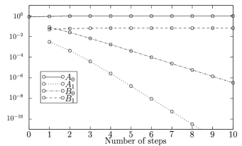
Figure 2: The evolution of the four parameters $A_{0},A_{1},B_{0}$, and $B_{1}$. Note that both $A_{1}$ and $B_{0}$ decrease exponentially fast in the number of steps.

To conclude this section, we summarize: For a large region $0.77184451\equiv f_{0}^{\mathrm{crit}}\leq f_{0}\leq 1$ the 2–EPP purifies and at the same time any eavesdropper is factored out. For a small region $0.75<f_{0}<f_{0}^{\mathrm{crit}}\equiv 0.77184451$, close to the threshold of the purification protocol, the conditional fidelity does not reach unity, while the protocol is in the purification regime. Even though the region is small and of little practical relevance (in this regime we are already out of the repeater regime Briegel et al. (1998) and purification is very inefficient), its existence shows that the process of factorization is an independent phenomenon and not trivially connected to EPP. A more exhaustive description of the intermediate regime will be published elsewhere.

III.3 Bell diagonal initial states

Now we want to show that the same result is true for arbitrary Bell diagonal states (Eq. (1)) and for noise of the form (4). The procedure is the same as in the case of binary pairs; however, a few modifications are required.

In order to keep track of the four different error operators $\sigma_{\mu}$ in (4), the lab demon has to attach two classical bits to each pair; let us call them the phase error bit and amplitude error bit. Whenever a $\sigma_{x}$ ($\sigma_{z}$, $\sigma_{y}$) error occurs, the lab demon inverts the error amplitude bit (error phase bit, both error bits). To update these error flags, he uses the update function given in Tab. 1). The physical reason for the choice of the flag update function will be given in the next section.

	(00)	(01)	(10)	(11)
(00)	(00)	(00)	(00)	(10)
(01)	(00)	(01)	(11)	(00)
(10)	(00)	(11)	(01)	(00)
(11)	(10)	(00)	(00)	(00)

Table 1: The value (phase error,amplitude error) of the updated error flag of a pair that is kept after a 2–EPP step, given as a function of the error flags of $P_{1}$ and $P_{2}$ (left to right and top to bottom, respectively).

Here, the lab demon divides all pairs into four subensembles, according to the value of their error flag. In each of the subensembles the pairs are described by a Bell diagonal density operator, like in Eq. (1), which now depends on the subensemble. That means, in order to completely specify the state of all four subensembles, there are 16 real numbers $A_{ij},B_{ij},C_{ij},D_{ij}$ with $i,j\in\{0,1\}$ required, for which one obtaines recurrence relations of the form

$$\begin{split}A^{(00)}_{n}&\rightarrow A^{(00)}_{n+1}(A^{(00)}_{n},A^{(01)}_{n},\ldots,D^{(11)}_{n}),\\ A^{(01)}_{n}&\rightarrow A^{(01)}_{n+1}(A^{(00)}_{n},A^{(01)}_{n},\ldots,D^{(11)}_{n}),\\ &\,\,\,\vdots\\ D^{(11)}_{n}&\rightarrow D^{(11)}_{n+1}(A^{(00)}_{n},A^{(01)}_{n},\ldots,D^{(11)}_{n}).\\ \end{split}$$ (11)

These generalize the recurrence relations (8) for the case of binary pairs, and the relations (2) for the case of noiseless apparatus.

Like the recurrence relations (2) and (8), respectively, these relations are (modulo normalization) quadratic forms in the 16 state variables $\vec{a}=\left(A^{(00)},A^{(00)},\ldots,D^{(11)}\right)^{T}$, with coefficients that depend on the error parameters $f_{\mu\nu}$ only. In other words, (11) can be written in the more compact form

$$\vec{a}^{\prime}_{j}=\vec{a}M_{j}\vec{a}^{T},$$ (12)

where, for each $j\in\{1,\ldots 16\}$, $M_{j}$ is a real $16\times 16$-matrix whose coefficients are polynomials in the noise parameters $f_{\mu\nu}$.

III.4 Numerical results

The 16 recurrence relations (11) imply a reduced set of 4 recurrence relations for the quantities $A_{n}=\sum_{ij}A_{n}^{(ij)},\ldots,D_{n}=\sum_{ij}D_{n}^{(ij)}$ which describe the evolution of the total ensemble (that is, the blend Englert (1999) of the four subensembles) under the purification protocol. Note that these values are the only ones which are known and accessible to Alice and Bob, as they have no knowledge of the values of the error flags. It has been shown in Briegel et al. (1998) that under the action of the noisy entanglement distillation process, these quantities converge towards a fixpoint $(A_{\infty},B_{\infty},C_{\infty},D_{\infty})$, where $A_{\infty}=F_{\text{max}}$ is the maximal attainable fidelity Dür et al. (1999).

Fig. 3 shows for typical initial conditions the evolution of the 16 coefficients $A_{n}^{(00)}\ldots D_{n}^{(11)}$. They are organized in a $4\times 4$-matrix, where one direction represents the Bell state of the pair, and the other indicates the value of the error flag. The figure shows the state (a) at the beginning of the entanglement purification procedure, (b) after few purification steps, and (c) at the fixpoint. As one can see, initially all error flags are set to zero and the pairs are in a Werner state with a fidelity of $70\%$. After a few steps, the population of the diagonal elements starts to grow; however, none of the elements vanishes. At the fixpoint, all off-diagonal elements vanish, which means that there are strict correlations between the states of the pairs and their error flags.

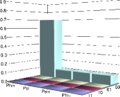
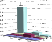
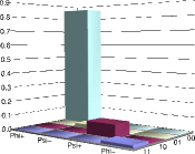
Figure 3: The evolution of the extended state

In order to determine how fast the state converges, we investigate two important quantities: the first is the fidelity $F_{n}\equiv A_{n}$, and the second is the conditional fidelity $F_{n}^{\text{cond}}\equiv A_{n}^{(00)}+B_{n}^{(11)}+C_{n}^{(01)}+D_{n}^{(10)}$. Note that the first quantity is the sum over the four $\left|\Phi^{+}\right\rangle$ components in Fig. 3, while the latter is the sum over the four diagonal elements. The conditional fidelity is the fidelity which Alice and Bob would assign to the pairs if they knew the values of the error flags, i. e.

$$F_{n}^{\text{cond}}=\sum_{i,j}\left\langle\Phi^{+}\right|\sigma_{i,j}\rho_{i,j}\sigma_{i,j}\left|\Phi^{+}\right\rangle,$$ (13)

where $\rho_{i,j}$ is the non-normalized state of the subensemble of the pairs with the error flag $(i,j)$. For convenience, we used the phase- and spin-flip bits $i$ and $j$ as indices for the Pauli matrices, i. e. $\sigma_{00}=\mathrm{Id},\sigma_{01}=\sigma_{x},\sigma_{11}=\sigma_{y},\sigma_{10}=\sigma_{z}$.

(a)                                         (b)

Figure 4: (a) The fidelities $F$ and $F_{\text{cond}}$ as a function of the number of steps in the entanglement distillation process (analytical results (lines) and Monte Carlo simulation (circles)). For the calculation, one and two qubit white noise with a noise fidelity of 97% has been assumed. The Monte Carlo simulation was started with 10000000 pairs; the numbers indicate how many pairs are left after each step of the distillation process. This decreasing number is the reason for the increasing fluctuations around the analytical curves.

The results that we obtain are similar to those for the binary pairs. We can also distinguish three regimes of noise parameters $f_{\mu\nu}$. In the high-noise regime (i. e., small values of $f_{00}$), the noise level is above the threshold of the 2–EPP and the fidelity $F$ and the conditional fidelity $F^{\mathrm{cond}}$ converge both to the value 0.25. In the low-noise regime (i. e., large values of $f_{00}$), F converges to the maximum fidelity $F_{\mathrm{max}}$ and $F^{\mathrm{cond}}$ converges to unity (see Fig. 4). This regime is the security regime, where we know that secure quantum communication is possible. Like for binary pairs, there exists also an intermediate regime, where the 2–EPP purifies but $F^{\mathrm{cond}}$ does not converge to unity. For an illustration, see Fig 5. Note that the size of the intermediate regime is very small, compared to the security regime. Whether or not secure quantum communication is possible in this regime is unknown. However, the answer of this question is irrelevant for all practical purposes, because in the intermediate regime the distillation process converges very slowly. A detailed discussion of the situation near the purification threshold will be published at some other place.

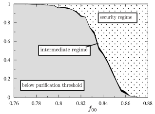
Figure 5: The size and the location of the three regimes of the distillation process. For fixed values of $f_{00}$, the remaining 15 noise parameters $f_{\mu\nu}$ have been choosen at random. Plotted is the relative frequency of finding the noise parameters in any of the three regimes as a function of $f_{00}$.

Even though the intermediate regime is practically irrelevant, it is important to estimate its size. For simplicity, we considered the case of one-qubit white noise, i.e. $f_{\mu\nu}=f_{\mu}f_{\nu}$ and $f_{1}=f_{2}=f_{3}=(1-f_{0})/3$. Here, this regime is known to be bounded by

$$0.8983<f^{\mathrm{crit,lower}}<f_{0}<f^{\mathrm{crit,upper}}<0.8988.$$

Regarding the efficiency of the distillation process, it is an important question how many initial pairs are needed to create one pair with the security parameter $\epsilon\equiv 1-F^{\text{cond}}$. Both the number of required initial pairs (resources) and the security parameter scale exponentially with the number of distillation steps, so that we expect a polynomial relation between the resources and the security parameter $\epsilon$. Fig. 6 shows this relation in a log-log plot for different noise parameters. The straight lines are fitted polynomial relations; the fit region is indicated by the lines themselves.

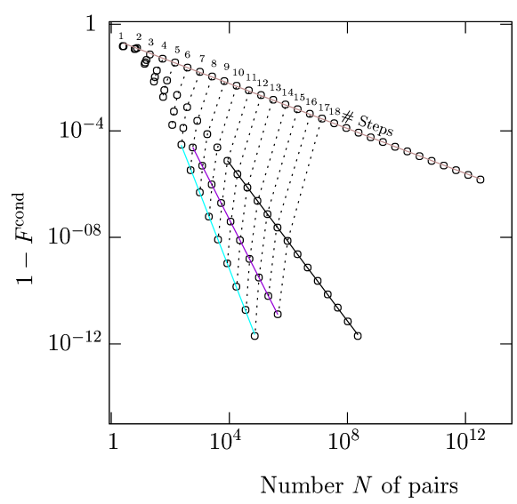
Figure 6: Number $N$ of pairs needed to create one pair with conditional fidelity $F^{\rm cond}$. The initial state of the pairs was of the Werner type with fidelity $F_{0}$ = 85%. One- and two-qubit errors were assumed with noise parameters $f_{1\rm bit}=f_{2\rm bit}=0.95,0.98,0.99,0.995$ (from top to bottom).

IV Discussion

We have shown in the preceeding section, that the two-way entanglement distillation process is able to disentangle any eavesdropper from Bell pairs distributed between Alice and Bob, even in the presence of noise, i. e. when the pairs can only be purified up to a specific maximun fidelity $F_{\mathrm{max}}<1$. Alice and Bob may use them as a secure quantum communication channel. They are thus able to perform secure quantum communication, and, as a special case, secure classical communication (which is in this case equivalent to a key distribution scheme).

In order to keep the argument transparent, we first considered the case where noise of the form (4) is explicitly introduced by a fictious lab-demon, who keeps track of all error operations and performs calculations. However, using a simple indistinguishability argument (see Section III.1), we could show that any apparatus with the noise characteristics (4) is equally secure as a situation where noise in introduced by the lab demon. This means that the security of the protocol does not depend on the fact whether or not anybody actually calculates the flag update function. It is sufficient to just use a noisy 2–EPP, in order to get a secure quantum channel.

For the proof, we had to make several assumptions on the noise that acts in Alices and Bobs entanglement purification device. One restriction is that we only considered noise which is of the form (4). However, this restriction is only due to technical reasons; we conjecture that our results are also true for most general noise models of the form (3). We have also implicitly introduced the assumption that the eavesdropper has no additional knowledge about the noise process, i. e. Eve only knows the publicly known noise characteristics (4) of the apparatus. This assumption would not be justified, for example, if the lab demon was bribed by Eve, or if Eve was able to manipulate the apparatus in Alice’s and Bob’s laboratories, for example by shining in light from an optical fiber. This concern is not important from a principial point of view, as the laboratories of Alice and Bob are considered secure by assumption. On the other hand, this concern has to be taken into account in any practical implementation.

References

- Bennett and Brassard (1985) C. H. Bennett and G. Brassard, in Proceedings of IEEE International Conference on Computers, Systems and Signal Processing, Bangalore, India (IEEE, New York, 1985), pp. 175–179.
- Ekert (1991) A. Ekert, Phys. Rev. Lett. 67, 661 (1991).
- Cirac et al. (1997) J. I. Cirac, P. Zoller, H. J. Kimble, and H. Mabuch, Phys. Rev. Lett. 78, 3221 (1997).
- Schumacher (1996) B. Schumacher, Phys. Rev. A 54, 2614 (1996).
- Mayers (1996) D. Mayers, in Advances in Cryptology – Proceedings of Crypto ’96 (Springer-Verlag, New York, 1996), pp. 343–357, see also quant-ph/9802025.
- Biham et al. (2000) E. Biham, M. Boyer, P. O. Boykin, T. Mor, and V. Roychowdhurny, in Proceedings of the Third-Second Annual ACM Symposium on Theory of Computing (ACM Press, New York, 2000), pp. 715–724, quant-ph/9912053.
- (7) H. Inamori, quant-ph/0008064.
- Shor and Preskill (2000) P. W. Shor and J. Preskill, Phys. Rev. Lett. 85, 441 (2000).
- Calderbank and Shor (1996) A. R. Calderbank and P. Shor, Phys. Rev. A 54, 1098 (1996).
- Deutsch et al. (1996) D. Deutsch, A. Ekert, R. Jozsa, C. Macchiavello, S. Popescu, and A. Sanpera, Phys. Rev. Lett. 77, 2818 (1996).
- Bennett et al. (1996a) C. H. Bennett, D. P. DiVincenzo, J. A. Smolin, and W. K. Wootters, Phys. Rev. A 54, 3824 (1996a).
- Bennett et al. (1992) C. H. Bennett, G. Brassard, and N. D. Mermin, Phys. Rev. Lett. 68, 557 (1992).
- Briegel et al. (1998) H.-J. Briegel, W. Dür, J. I. Cirac, and P. Zoller, Phys. Rev. Lett. 81, 5932 (1998).
- Dür et al. (1999) W. Dür, H.-J. Briegel, J. I. Cirac, and P. Zoller, Phys. Rev. A 59, 169 (1999).
- Giedke et al. (1999) G. Giedke, H.-J. Briegel, J. I. Cirac, and P. Zoller, Phys. Rev. A 59, 2641 (1999).
- Lo and Chau (1999) H.-K. Lo and H. F. Chau, Science 283, 2050 (1999).
- Bennett et al. (1996b) C. H. Bennett, G. Brassard, S. Popescu, B. Schumacher, J. A. Smolin, and W. K. Wootters, Phys. Rev. Lett. 70, 722 (1996b).
- Macchiavello (1998) C. Macchiavello, Phys. Lett. A 246, 385 (1998).
- (19) H. Aschauer and H.-J. Briegel, eprint quant-ph/0008051.
- Kraus (1983) K. Kraus, States, Effects, and Operations, vol. 190 of Lecture Notes in Physics (Springer Verlag, Berlin Heidelberg New York Tokyo, 1983).
- Englert (1999) B.-G. Englert, Z. Naturforsch. 54a, 11 (1999).