Proceedings ICSSUR2001
Is “entanglement” always entangled?
Abstract
Entanglement, including “quantum entanglement,” is a consequence of correlation between objects. When the objects are subunits of pairs which in turn are members of an ensemble described by a wave function, a correlation among the subunits induces the mysterious properties of “cat-states.” However, correlation between subsystems can be present from purely non-quantum sources, thereby entailing no unfathomable behavior. Such entanglement arises whenever the so-called “qubit space” is not afflicted with Heisenberg Uncertainty. It turns out that all optical experimental realizations of EPR’s Gedanken experiment in fact do not suffer Heisenberg Uncertainty. Examples will be analyzed and non-quantum models for some of these described. The consequences for experiments that were to test EPR’s contention in the form of Bell’s Theorem are drawn: valid tests of EPR’s hypothesis have yet to be done.
pacs:
03.65.Bz, 03.67.-a, 41.10.Hv, 42.50.ArI Introduction
The above title needs ‘disentanglement.’ The quantum wave function of entangled, i.e., of correlated subsystems, can not be written as the product of the wave functions for the subsystems. Likewise the probability of correlated events can not be written as the product of probabilities for two independent events. The latter fact is elementary and very well understood; it presents absolutely no mystery, but in Quantum Mechanics (QM), on the contrary, the same fact is utterly impenetrable.
What is the difference?
It arises from the following considerations. In probability theory, the probability for joint events is given in general by Bayes’ formula:
| (1) |
where is the conditional probability that the event occurs given that event has been seen.wf This is a statement about the knowledge that the observer has about the joint events; it is an epistemological statement, and, as such, the dependance of on is devoid of communicative implications. Now, in QM, according to the Born interpretation, the modulus squared of a wave function, i.e. , is the probability that the object to which it pertains will be found in the infinitesimal volume . This straightforward concept is complicated, however, by the peculiarity of QM, namely, a wave function is known empirically to diffract at boundaries, just like water or electromagnetic waves, and this seems to make sense only if wave functions have ontological substance. In turn, this appears to vest a causative relationship into conditional probabilities computed from wave functions for correlated events. In short, entanglementQM is somehow ontological, but entanglementProb, epistemological. In this light the title is: Is (in the microscopic domain) entanglementProb always entangledQM? The purpose of this report is to argue that in virtually all of the crucial experimental tests of Bell’s Theorem, the answer is: no!
Born’s interpretation of the wave function has led many, in particular Einstein, Podolsky and Rosen (EPR), to argue that the necessity for probabilistic concepts in QM arises because the theory is limited fundamentally by ignorance; i.e., that QM should be ‘extendable,’ at least in principle, so as to encompass the heretofore missing information, perhaps using “hidden variables.” The tactic taken by EPR was to show that ‘Heisenberg Uncertainty’ is not something novel, that is, that basic logic regarding correlated objects demands that the missing information be due to simple ignorance. This they did by considering the symmetrical disintegration of a stationary particle into twin daughters. For each daughter separately, the Heisenberg Uncertainty Principle implies that both the position and momentum can not be simultaneously known to arbitrary precision. Some go on to argue that this is so because they in fact do not exist simultaneously. EPR countered, arguing (in the author’s rendition) that in the case of such a disintegration one can measure the position of one daughter and the momentum of the other to arbitrary precision and thereafter call on symmetry to specify to equal precision the momentum of the first and position of the second. What can be specified in principle to arbitrary precision, EPR argued, must be an “element of reality” that enjoys ontological status. In any case, EPR intended that their Gedanken experiment should expose the ultimate character of Heisenberg Uncertainty, that it is ultimately just ignorance, not something fundamentally new.epr
For the purposes of an experimental realization of EPR’s Gedanken experiment, however, the difficulties finding a suitable source of the sort envisioned, are daunting. Thus, Bohm proposed a change of venue; instead of momentum-position, he suggested using the (anti)correlated spin states derived from a mother with no net angular momentum.db His motivation, apparently, was that it should be easier to construct an appropriate source, and easier to measure the dichotomic values of the daughters. Ultimately, this proposal too turned out to be impractical, but the algebraically isomorphic situation with polarized ‘photons’ from a cascade transition or from parametric down conversion is workable and a several such experiments have been done.as
II EntanglementQM vs. entanglementProb
It is the fundamental premise of this report that Bohm’s transfer of venue introduced a major error. It is the following: the space of the variables for either spin or polarization, contrary to phase space where EPR formulated their Gedanken experiment, is not afflicted by Heisenberg Uncertainty (HU). There is no HU in the plane of the spin or polarization vector. Neither nor { are Hamiltonian canonically conjugate variables; their creation and annihilation operators commute. Anticommutation of spin operators here arises for the same reason it does for angular momentum operators in classical mechanics. Thus, while they do share some of the characteristics of the variables of phase space, they do not share the one relevant for the argument of EPR.
This fact has a number of immediate consequences, the most salient of which is that probabilities of these variables do not exhibit the quantum phenomena that ultimately demands that QM probabilities have an ontological character. This means, in particular, that conditional probabilities of these variables do not imply causality. Thus, Bell’s argument that because there is to be no causal relationship between the two detection events, the probability relationship between them can not take the form
| (2) |
which, in turn, implies that Eq. (1) must read jb , does not follow for these experiments, because, in fact there need be no causative link between these variables.as In other words, Bell’s encoding of “locality” with respect to these variables is not justified in these circumstances. A conditional probability involving a state of polarization as a ‘condition’ is an epistemological statement about the state of knowledge, not an ontological statement about EPR’s “elements of reality.” This follows directly from the fact that there is no reason whatsoever to attribute physical interference between polarization states, these states are simply orthogonal from the start and do not interact. In short, statements about joint probabilities between such states do not imply any causal relationships; the non-factorizability of their wave function is no more problematic than that of probabilities of correlated events.
III Non-quantum models of EPR-B experiments
In view of the facts developed above, which imply that experiments exploiting polarization that are intended to test EPR (or Bell inequalities), in so far as they are not cast in a space suffering HU, should be modelable classically. This is indeed the case, and the most common types of EPR-B experiments are presented below. These include both those based on polarization and a second category in which orthogonality of the signals is achieved by other means, usually as pulses with a phase offset. This latter category includes the ‘Franson,’ ‘Ghosh and Mandel’ and ‘Suarez-Gisin’ type experiments.
III.1 ‘Clauser-Aspect’ type experiments
In these experiments the source is a vapor, typically of mercury or calcium, in which a cascade transition is excited by either an electron beam or an intense radiation beam of fixed orientation. Each stage of the cascade results in emission of radiation (a “photon”) that is polarized orthogonally to that of the other stage. In so far as the sum of the emissions can carry off no net angular momentum, the separate emissions are antisymmetric in space. The intensity of the emission is maintained sufficiently low so that at any instant the likelihood is that radiation from only one atom is visible. Photodetectors are placed at opposite sides of the source, each behind a polarizer with a given setting. The experiment consists of measuring the coincidence count rate as a function of the polarizer settings.ch
A model consists of simply rendering the source and polarizers mathematically, and a computation of the coincidence rate. Photodetectors are assumed to convert continuous radiation into an electron current at random times with Poisson distribution but in proportion to the intensity of the radiation. The coincidence count rate is taken to be proportional to the fourth order coherence function evaluated at the detectors.
The source is assumed to emit a double signal for which individual signal components are anticorrelated and, because of the fixed orientation of the excitation source, confined to the vertical and horizontal polarization modes; i.e.
| (3) |
where takes on the values and with an even, random distribution. The transition matrix for a polarizer is given by,
| (4) |
so the fields entering the photodetectors are given by:
| (5) |
Coincidence detections among photodetectors (here ) are proportional to the single time, multiple location second order cross correlation, i.e.:
| (6) |
It is shown in Coherence theory that the numerator of Eq. (6) reduces to the trace of , the system coherence or “polarization” tensor.mw It is easy to show that for this model the denominator consists of constants and will be ignored as we are interested only in relative intensities. The final result of the above is:
| (7) |
This is immediately recognized as the so-called ‘quantum’ result. (Of course, it is also Malus’ Law, thereby being in total accord with the premise of this report.)
III.2 ‘GHZ’ experiments
A number of proposed experiments involving more that two particles, many stimulated by analysis of Greenburger, Horne and Zeilinger (GHZ), are expected to reveal QM features with particularly alacrity.ghz One of the most recent, which has the great virtue of being experimentally doable, is that performed by Pan et al.pd See Fig. (1). Two independent signal pairs are created by down-conversion in a crystal pumped by a pulsed laser. The laser pulse passes through the crystal creating one pair then is reflected off a movable mirror to repass through the crystal in the opposite direction creating a second pair. One signal from each pair is fed directly through polarizers to photodetectors (signals and . The other signal from each pair and is directed to opposite faces of a PBS, (i.e., a beam splitter which reflects vertically and transmits horizontally polarized signals) after which the signals are passed through adjustable polarizers into photodetectors. The path lengths of signals 2 and 3 are adjusted so as to compensate for the time delay in the creation of the pairs. By moving the mirror, the compensation can be negated to permit studying the coincidence dependence on the degree of interference caused by simultaneous “cross-talk” between channels 2 and 3.

The principle results reported in Ref. pd are the following. Of all the 16 possible regimes setting: , only and yield a (substantial) four-fold coincidence count, ; the regime occurs with an intensity and the regime with zero intensity. Further, both of the later regimes yield an intensity of when the time between pair creation is so large that that there is no “cross-talk” between channels 2 and 3.
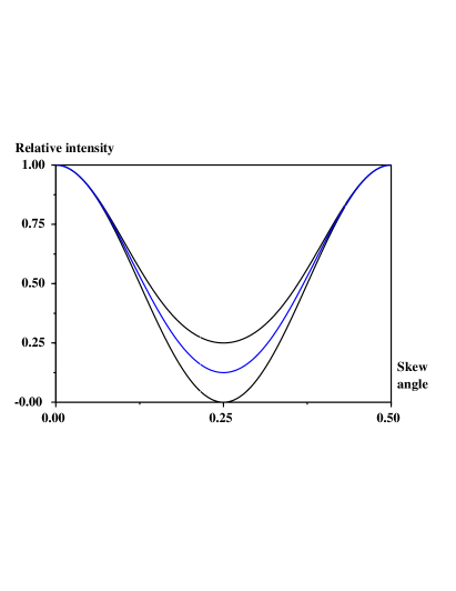
Eq. (6) was implemented as follows: The crystal is assumed to emit a double signal for which individual signal components are anticorrelated and confined to the vertical and horizontal polarization modes; i.e.
| (8) |
where and take the values and randomly. The polarizing beam splitter (PBS) is modeled using the transition matrix for a polarizer, , Eq. (4) where accounts for a reflection and a transmission. Thus the final field impinging on each of the four detectors is :
| (9) |
which, using Eq. (6), does not result in a simple expression. However, it can be numerically computed easily to obtain the same results as reported by Pan et al., or extended to other regimes, such as that shown in Fig. (2).
III.3 ‘Franson’ experiments
Experiments of this type exploit phase shifts between pulses in the form of time offsets to define the orthogonal states played by the two states of polarization in the setups described above.jf The original ‘Franson’ experiment measures the correlation between two detectors positioned after interferometers which divide identical incoming pulses such that half takes a short route and half takes a long root which includes an adjustable delay. See Fig. (3).

There are two means of modeling this setup. One would be to write out terms for the long- and short-route pulses that had time-separated modulation or time-limited coherence. This approach has the disadvantage of leading ungainly expressions. A much simpler tactic is to assign the signals in the long and short paths to orthogonal dimensions of a vector space; the resulting calculations are then transparent and devoid of gratuitous complexity. For example:
| (10) |
where and are the extra phase shifts introduced in the long paths. Then, using Eq. (6), with the convention that the tensor product be replaced by a vector inner product; i.e.,
| (11) |
(to algebraically enforce the orthogonality in calculations that phase shifts enforce in the experiment) directly gives the observed correlation as a function of the phase shifts:
| (12) |
which exhibits the oscillation with visibility characteristic of idealized versions of these experiments.
‘Ghosh-Mandel’ type experiments are a variation of the ‘Franson’ version in which the phase shift is achieved by path-length differences instead of time-offsets; otherwise, the formulas are identical.GM
III.4 ‘Brendel’ experiments
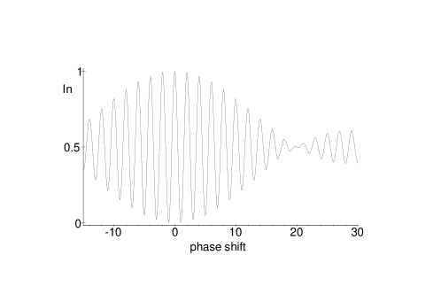
In the above experiment the radiation source was taken to be ideal, that is, it produced two signals of exactly the same frequency with no dispersion. In some experiments, bm the source used was a nonlinear crystal generating two correlated but not necessarily identical pulses, which satisfy ‘phase matching conditions’ so that if one signal in frequency is above the mean by (spread), the other is down in frequency by the same amount. This leads to an additional phase shift at the detectors which is also proportional to those already there; i.e., and , so that:
| (13) |
Since the value of is different for each pulse (photon) pair, the resulting signal is an average over the relevant values of :
| (14) |
where is computed as for ‘Franson’ experiments. The final result closely matches that observed by Brendel et al. See Fig. (4).
III.5 ‘Suarez-Gisin’ experiments
In experiments of this type, one of the detectors is set in motion relative to the other. By doing so with appropriately chosen parameters, it is possible to arrange the situation such that each detector precedes the other in its own frame.gs Thus, not only is the ‘collapse’ of the wave packet “nonlocal,” it occurs such that there is also “retrocausality.” In the model proposed herein, however, this complication (paradox) can not arise in the first instance. All the properties of each pulse are determined completely at the common point at which the signals are generated. Properties measured at one detector in no way determine those at other detectors, regardless of the order in which an observer receives reports of the results from various detectors, and regardless of what conditional probabilities he might write to describe his hypothetical or real knowledge.
IV Conclusion
The model or explanation of the experiments described above is fully classical. It uses no special property peculiar to QM. The two states in these experiments (polarization or phase-displaced pulses) are not canonically conjugate dynamical variables; they do not, therefore, exhibit Heisenberg Uncertainty, and the model does not bring any in. The essential formulas are a straightforward application of second order (in intensity) coherence theory, which is really just a generalization of wave interference. That this model faithfully describes the outcomes of these experiments, in addition to being a counterexample to claims that these experiments can not be clarified using non-quantum physics, is a demonstration that they are not relevant to EPR’s argumentation, and therefore, that to date no such experiment could have established that non-locality has a role to play in the explanation of the natural world. It shows that there is no justification for ascribing an ontological meaning to conditional probabilities in the circumstances of these experiments, which, in turn, undermines the rationale for Bell’s encoding of non-locality. When his encoding is withdrawn, no Bell inequality can be extracted.
There are, of course, two arenas where HU is in evidence: phase space and ‘quadrature space.’ In principle, a test of EPR’s contentions formulated in these arenas could show different results — at least in so far as the considerations herein are germane.
To a large extent, the model proposed herein is ‘obvious.’ It might be asked: why has it not been proposed then long ago? The answer involves issues resulting from the perceived need to maintain an ontological ambiguity with respect to the identity of wave functions until the moment of measurement, at which time this identity ambiguity is resolved by a “collapse.” This need results from the tactic of describing particle beams with wave functions in order to account for their wave-like diffraction. That is, the wave-like navigation of particle beams in combination with their incontestable particle-like registration in detectors, has been explained, or at least encoded, calling on ‘dualism,’ ‘wave-collapse’ and so on.ak The experiments described herein, however, employ optical phenomena for which there is no need to invoke a particulate character. Wave beams diffract naturally. And, particulateness in detectors can be, indeed must be, attributed to the fact that photodetectors, because of the discrete nature of electrons, convert continuous radiation into a digitized photocurrent. The conceptual contraptions of ‘duality’ and ‘collapse’ are just not needed to explain the behavior of radiation beams, even correlated sub beams. There is no reason these experiments could not be carried out in spectral regions in which it is possible to track the time development of electromagnetic fields thereby avoiding the peculiarities of photodetectors. In fact, for simple ‘Clauser-Aspect’ type setups, this has been done.ek The results conform with ours and show that classical optics is not taxed to clarify EPR-B correlations.
Note: An e-file with MAPLE routines for the above is available upon request.
References
- (1) W. Feller, An Introduction to Probability Theory and its Applications (John Wiley & Sons, New York, 1950) Chapter V.
- (2) A. Einstein, B. Podolsky N. and Rosen, Phys. Rev. 47, 777 (1935).
- (3) D. Bohm, Quantum Theory, (Prentice-Hall, New York, 1951).
- (4) A. Afriat and F. Selleri, The Einstein, Podolsky and Rosen Paradox, (Plenum, New York, 1999) review both the theory and experiments from a current prospective.
- (5) J. S. Bell, Speakable and unspeakable in quantum mechanics, (Cambridge University Press, Cambridge, 1987).
- (6) J. F. Clauser and M. A. Horne, Phys. Rev. D10, 526 (1974). A. Aspect et al. Phys. Rev. Lett. 47, 460 (1981), 49, 91 (1982), 49, 1804 (1982).
- (7) L. Mandel and E. Wolf, Optical Coherence and Quantum Optics (Cambridge University Press, Cambridge, 1995) p. 447.
- (8) D. M. Greenburger, M. Horne and A. Zeilinger, in Bell’s Theorem, Quantum Theory and Conceptions of the Universe, M. Kafatos ed., (Kluwer, Dordrecht, 1989), p. 73.
- (9) J.-W. Pan, M. Daniell, S. Gasparoni, G. Weihs and A. Zeilinger, Phys. Rev. Lett. 86, 4435 (2001).
- (10) J. D. Franson, Phys. Rev. Lett. 62, 2205 (1989). R. Ghosh and L. Mandel, Phys. Rev. Lett. 59, 1903 (1987).
- (11) R. Ghosh and L.Mandel, Phys. Rev. Lett. 59, 1903 (1987).
- (12) J. Brendel, E. Mohler and W. Martienssen, Europhys. Lett. 20 (7), 575 (1992).
- (13) N. Gisin, V. Scarani, W. Tittle, and H. Zbinden, http://arXiv:quant-ph/00 09 055. A. Suarez, Phys. Lett. A236, 383 (1997).
- (14) A. F. Kracklauer, Found. Phys. Lett. 12 (5) 441 (1999) describes a classical paradigm rationalizing particle beam “duality.”
- (15) N. V. Evdokimov, D. N. Klyshko, V. P. Komolov and V. A. Yarochkin, Physics - Uspekhi 39, 83 (1996).