Quantum cryptography using photon source based on postselection from entangled two-photon states

Abstract

A photon source based on postselection from entangled photon pairs produced by parametric frequency down-conversion is suggested. Its ability to provide good approximations of single-photon states is examined. Application of this source in quantum cryptography for quantum key distribution is discussed. Advantages of the source compared to other currently used sources are clarified. Future prospects of the photon source are outlined.

Keywords: single-photon source, quantum cryptography, quantum key distribution, down-conversion, postselection, entanglement

PACS: 03.67.Dd - Quantum cryptography, 42.50.Dv - Nonclassical field states,…, 42.65.Ky - Harmonic generation,…

I Introduction

Entangled photon pairs produced by spontaneous parametric frequency down-conversion [1, 2] have recently been widely used in experimental quantum physics. They have been successfully applied in the research of fundamental problems of quantum theory [3]. Among others, a direct application of nonclassical properties of such states in optical communications has been suggested [4] in 1991.

Since then the area of quantum communications underwent an immense progress. Quantum key distribution (QKD) became a well understood scheme for establishing a provably secure shared secret not only at a theoretical level. Experimental realization brought QKD at the disposal of future commercial applications [5]. Most of the practical QKD schemes designed until now relied on dim coherent pulses as a carrier of qubits. While this scheme suffers from the lack of the ultimate proof of security [6, 7], its security is very well defined and understood [8].

Recently, the idea to use correlated photon pairs for QKD has been revisited in two different ways. First, the laboratory realization of the original Ekert’s protocol has been improved and modified [9, 10, 11, 12] and its security has been addressed [13]. A passive scheme for choosing from two possible transmission bases has been suggested and realized. Possibility of multiphoton attacks on QKD is substantially reduced in this scheme. Second, the fact that down-converted photons are always produced in pairs has been used to suggest a new source of photons applicable in quantum cryptography [8, 14, 15]. The state describing such correlated fields cannot be factorized into a product of states of signal and idler beams. When a measurement is performed on one of the beams, the whole state including the other beam is changed. When a photon is detected in, e.g., the signal beam, we know that its twin must be present in the idler beam. This suggests to construct a single-photon source as follows: Perform a photon-number measurement on one of the beams and select only those cases when a single photon has been detected. Then there is a single photon in the other beam with a high probability and this photon is used for cryptography. Filtering of both vacuum and multiphoton states contributes to the security of QKD. Moreover, as is shown in the paper, this scheme provides higher values of transmission rates. A passive scheme that lowers the vulnerability to multiphoton attacks may also be implemented in this case.

Practical existence of a one-photon source would help formulating general security proofs [6] of quantum key distribution protocols in secure quantum cryptography. It would also make practical schemes more efficient [8].

A realistic model of such source of photons including imperfections encountered in the laboratory is developed in the paper. Efficiency of the postselection procedure as well as applicability of the source in real quantum cryptography are discussed.

II Model of the source

We assume that a postselection device is placed in the signal beam. This device yields a simple yes-no result (a trigger) and, based on this result, the state in the idler beam is either coupled to the transmission line or rejected. It is, however, not an easy task to construct a practical photon-number measuring device. Generally used photon-counting detectors (avalanche photodiodes or photomultipliers) use many-order noisy amplification processes that smear out resolution of small photon numbers. In our work we use a model of a photon number measuring device based on $1\times N$ coupler [16]. We note, that novel detectors capable to resolve small numbers of photons and sources of single photons occured recently [17]. However, they work only at very low temperatures and having practical QKD on mind, we do not consider them here. Performance of a measuring device based on $1\times N$ coupler and $N$ detectors and a photon-number resolving detector in the preparation of a state in postselection procedure has been studied in [18].

In our model [15, 19] we assume that the down-conversion process is pumped by either cw or pulsed laser beam. The signal and idler beams are selected by filters and pinholes (geometrically and spectrally filtered). The filtering is in general imperfect, i.e. sometimes only one of the members of the pair reaches a detector. Detectors have limited quantum efficiencies and they are not capable of resolving the photon number, they just click in the presence of the signal containing one or more photons. In addition, there are noise detections coming both from dark counts of the detectors and from stray light in the laboratory. The scheme including all these imperfections is given in Fig. 1.

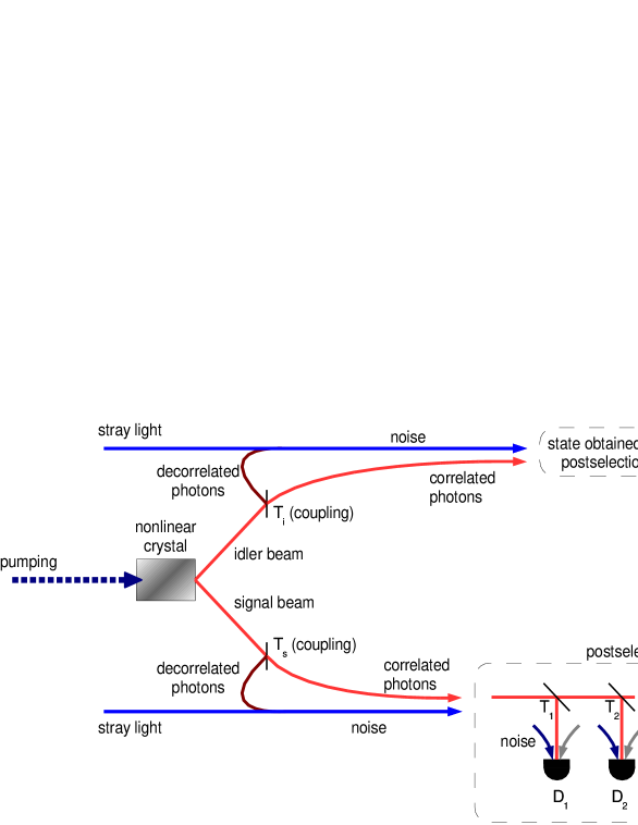
FIG. 1.: Scheme of the model. Photons of the pump beam are split in the nonlinear crystal to pairs of mutually entangled photons. The signal beam is then coupled to a postselection device consisting of a $1\times N$ coupler and $N$ detectors ($T_{i}$ stands for the intensity transmission coefficient to $i$th detector, $T_{i}=|t_{i}|^{2}$). Coupling is imperfect and decorrelated photons contribute to the noise impinging on the detectors that exhibit also internal dark-count noise. The idler beam suffers similar coupling problems.

Detection of a photoelectron is described by the following projection operator ($\eta$ is quantum efficiency of the detector):

$$\hat{P}^{\rm det}=\sum_{n=1}^{\infty}\left[1-\left(1-\eta\right)^{n}\right]\left|n\right\rangle\left\langle n\right|+d\!\sum^{\infty}_{n=0}\left(1-\eta\right)^{n}\left|n\right\rangle\left\langle n\right|,$$ (1)

where $d$ represents a total noise count rate determined as

$$d=d^{\rm dark}+\left(1-d^{\rm dark}\right)\!d^{\rm noise},$$ (2)

when both dark counts and noise coming from stray light and decorrelated photons are taken into account (for details, see Appendix A). The projection operator $\hat{P}^{\rm nodet}$ appropriate in the case when a photoelectron does not occur in the detector has the form ($\hat{P}^{\rm nodet}=\hat{1}-\hat{P}^{\rm det}$):

$$\hat{P}^{\rm nodet}=\left(1-d\right)\!\sum^{\infty}_{n=0}\left(1-\eta\right)^{n}\left|n\right\rangle\left\langle n\right|.$$ (3)

The light field emerging from the output of the nonlinear crystal is in an entangled multimode state. However, it can be described as an entangled state of two effective modes (one for the signal field, the other for the idler field) by the statistical operator $\hat{\rho}_{S,I}$:

$$\hat{\rho}_{SI} = |\psi\rangle\langle\psi|,$$ (4)

$$|\psi\rangle = \sum_{n=0}^{\infty}c_{n}|n,n\rangle_{S,I}\!,$$ (5)

where the indices $S$ and $I$ refer to the signal and idler beams, respectively. As is shown in Appendix B, the statistics of pairs of photons in two effective modes is Poissonian, i.e.:

$$\left|c_{n}\right|^{2}=\frac{\mu^{n}}{n!}e^{-\mu},$$ (6)

$\mu$ being the mean number of pairs generated during a detection interval.

Both the signal and idler beams experience losses before they are detected (spectral filtering by interference filters, geometrical filtering by pinholes and other elements in the experimental setup). We represent all these losses by quantally described beamsplitters [20]; a beamsplitter in the signal (idler) field has a transmission coefficient $T_{S}$ ($T_{I}$). Diagonal elements of the statistical operator $\hat{\rho}^{\prime}_{S,I}$ in the Fock-state basis then have the form (the signal and idler fields are partially decorrelated; $R_{S}=1-T_{S}$, $R_{I}=1-T_{I}$):

$$(\hat{\rho^{\prime}}_{S,I})_{l_{S}l_{I},l_{S}l_{I}}=\sum_{n={\rm max}(l_{S},l_{I})}^{\infty}|c_{n}|^{2}\left(\begin{array}[]{c}n\\ l_{S}\end{array}\right)T_{S}^{l_{S}}R_{S}^{n-l_{S}}\left(\begin{array}[]{c}n\\ l_{I}\end{array}\right)T_{I}^{l_{I}}R_{I}^{n-l_{I}},$$ (7)

where the symbol ${\rm max}$ denotes the maximum function. We limit ourselves only to the determination of diagonal elements of the statistical operator $\hat{\rho^{\prime}}_{S,I}$, because they are sufficient for the description of the detection process.

Photon-number measurement in the signal field may be approximatelly reached using a $1\times N$ coupler and $N$ detectors. Provided that the mean photon number of the signal field is much lower that the number of detectors and the detectors exhibit moderate quantum efficiencies and dark count rates, only one detector detects a photon on single-photon signal while multiple detections occur on multi-photon signals with high probability. A $1\times N$ coupler is described by the unitary transformation,

$$\hat{a^{\prime}}_{S}=\sum_{j=1}^{N}t_{j}\hat{a}_{j},$$ (8)

where $\hat{a^{\prime}}_{S}$ stands for the annihilation operator at the input of the coupler, $\hat{a}_{j}$ is the annihilation operator at the $j$-th output of the coupler, and $t_{j}$ means the amplitude transmission coefficient of a photon propagating from the input to the $j$-th output of the coupler ($j=1,\ldots,N$).

The statistical operator $\hat{\rho}^{\rm post}_{I,k}$ describing the idler field after a signal photon has been detected at the $k$-th detector and no photon has been detected at all other detectors beyond the $1\times N$ coupler is determined as follows:

$$\hat{\rho}^{\rm post}_{I,k}=\frac{{\rm Tr}_{S}(\hat{\rho^{\prime}}_{S,I}\hat{P}^{\rm det}_{k}\prod_{j=1,\ldots,N;j\neq k}\hat{P}^{\rm nodet}_{j})}{{\rm Tr}_{S,I}(\hat{\rho^{\prime}}_{S,I}\hat{P}^{\rm det}_{k}\prod_{j=1,\ldots,N;j\neq k}\hat{P}^{\rm nodet}_{j})},$$ (9)

where the projection operators $\hat{P}^{\rm det}_{j}$ given in Eq. (1) and $\hat{P}^{\rm nodet}_{j}$ defined in Eq. (3) are related to the $j$-th detector. Using the statistical operator $\hat{\rho^{\prime}}_{S,I}$ given in Eq. (6) together with the relation appropriate for the $1\times N$ coupler in Eq. (7), we arrive at the expression:

$$(\hat{\rho}^{\rm post}_{I,k})_{l_{I},l_{I}} = \frac{1}{r_{I,k}}\left\{\left[\prod_{l=1,\ldots,N;l\neq k}(1-d_{l})\right]\sum_{n=l_{I}}^{\infty}|c_{n}|^{2}\left(\begin{array}[]{c}n\\ l_{I}\end{array}\right)T_{I}^{l_{I}}R_{I}^{n-l_{I}}{\cal A}_{k}^{n}\right.$$ (15)

$$\mbox{}-\left.\left[\prod_{l=1}^{N}(1-d_{l})\right]\sum_{n=l_{I}}^{\infty}|c_{n}|^{2}\left(\begin{array}[]{c}n\\ l_{I}\end{array}\right)T_{I}^{l_{I}}R_{I}^{n-l_{I}}{\cal B}^{n}\right\},$$

and

$${\cal A}_{k} = R_{S}+T_{S}\left(|t_{k}|^{2}+\sum_{l=1,\ldots,N;l\neq k}|t_{l}|^{2}(1-\eta_{l})\right),$$ (16)

$${\cal B} = R_{S}+T_{S}\left(\sum_{l=1}^{N}|t_{l}|^{2}(1-\eta_{l})\right).$$ (17)

The symbol $\eta_{j}$ stands for the quantum efficiency of the $j$-th detector. The normalization constant $r_{I,k}$ is determined as follows:

$$r_{I,k}=\left[\prod_{l=1,\ldots,N;l\neq k}(1-d_{l})\right]\sum_{n=0}^{\infty}|c_{n}|^{2}{\cal A}_{k}^{n}-\left[\prod_{l=1}^{N}(1-d_{l})\right]\sum_{n=0}^{\infty}|c_{n}|^{2}{\cal B}^{n}.$$ (18)

Noise in the signal beam coming from both stray light and decorrelated photons may be included into the model through the constants $d^{\rm noise}$ in Eq. (2). The influence of noise in the idler beam has to be described more precisely. We consider a chaotic field with the statistical operator $\hat{\rho}_{I,k}^{\rm res}$ (for details, see Appendix B) statistically independent on the idler field stemming from the postselection procedure. The statistical operator $\hat{\rho}^{\rm mix}_{I,k}$ of the overall field at the detector in the idler beam is given as follows [21]:

$$\hat{\rho}_{I,k}^{\rm mix}=\sum_{n=0}^{\infty}|n\rangle_{I}{}_{I}\langle n|\sum_{m=0}^{n}(\hat{\rho}_{I,k}^{\rm post})_{m,m}(\hat{\rho}_{I,k}^{\rm res})_{n-m,n-m}.$$ (19)

We now consider Poissonian statistics of the generated pairs of photons (the coefficients $c_{n}$ are given in Eq. (5)) and chaotic noisy fields both in the signal and idler beams (see Appendix B):

$$(\hat{\rho}_{I,k}^{\rm res})_{n,n} = (1-\nu^{\rm res}_{I,k})(\nu^{\rm res}_{I,k})^{n},\hskip 14.22636pt\nu^{\rm res}_{I,k}=\frac{\mu^{\rm res}_{I,k}}{1+\mu^{\rm res}_{I,k}},$$ (20)

$$(\hat{\rho}_{S,j}^{\rm res})_{n,n} = (1-\nu^{\rm res}_{S,j})(\nu^{\rm res}_{S,j})^{n},\hskip 14.22636pt\nu^{\rm res}_{S,j}=\frac{\mu^{\rm res}_{S,j}}{1+\mu^{\rm res}_{S,j}},\hskip 14.22636ptj=1,\ldots,N.$$ (21)

The symbol $\mu_{I,k}^{\rm res}$ denotes the mean number of noisy photons in the idler beam and $\mu^{\rm res}_{S,j}$ is the mean number of noisy photons in the signal field at the $j$-th detector. The diagonal matrix elements of the statistical operator $\hat{\rho}_{I,k}^{\rm mix}$ given in Eq. (12) then take the form:

$$(\hat{\rho}_{I,k}^{\rm mix})_{nn} = \frac{1-\nu^{\rm res}_{I,k}}{\exp(-\mu{\cal B})-(1-d_{k})\exp(-\mu{\cal A}_{k})}$$ (24)

$$\mbox{}\times\left\{\exp(-\mu{\cal B})\exp(-\mu{\cal A}_{k}T_{I})(\nu_{I,k}^{\rm res})^{n}f_{n}\left(\frac{\mu{\cal A}_{k}T_{I}}{\nu_{I,k}^{\rm res}}\right)\right.$$

$$\left.\mbox{}-(1-d_{k})\left[\exp(-\mu{\cal A}_{k})\exp(-\mu{\cal B}T_{I})(\nu_{I,k}^{\rm res})^{n}f_{n}\left(\frac{\mu{\cal B}T_{I}}{\nu_{I,k}^{\rm res}}\right)\right]\right\},$$

and

$$f_{n}(x)=\sum_{l=0}^{n}\frac{x^{l}}{l!}.$$ (26)

The normalization constant $r_{I,k}$ is determined according to:

$$r_{I,k}=\left[\prod_{l=1,\ldots,N;l\neq k}(1-d_{l})\right]\exp[-\mu(1-{\cal A}_{k})]-\left[\prod_{l=1}^{N}(1-d_{l})\right]\exp[-\mu(1-{\cal B})].$$ (27)

The noisy field in the signal beam is given by the photons that lost their twins (the term $T_{S}\mu$ in Eq. (17) below, see Appendix C for details) and by additional noisy photons coming, e.g., from stray light (the mean number of additional noisy photons is denoted as $\mu^{\rm res,add}_{S}$). We then have:

$$\mu^{\rm res}_{S,j}=|t_{j}|^{2}\mu^{\rm res}_{S};\hskip 28.45274pt\mu^{\rm res}_{S}=(T_{S}\mu+\mu^{\rm res,add}_{S}).$$ (28)

The constants $d^{{\rm noise}}_{j}$ in Eq. (2) describing the influence of noise in the signal beam at the $j$-th detector are then determined as follows:

$$d^{\rm noise}_{j}=\frac{\eta_{j}\mu^{\rm res}_{S,j}}{1+\eta_{j}\mu^{\rm res}_{S,j}}.$$ (29)

Similarly, assuming that the noisy field in the idler beam consists of both idler photons without their twins in the signal field and additional noisy photons with the mean number of photons denoted as $\mu^{\rm res,add}_{I}$, we have:

$$\mu^{\rm res}_{I,k}=T_{I}\mu+\mu^{\rm res,add}_{I}.$$ (30)

If narrow spectra of the down-converted fields are considered, the statistics of generated pairs is given by the Bose-Einstein distribution [2]. Relations valid in this case can be found in Appendix D.

We further consider a symmetric $1\times N$ coupler and $N$ identical detectors:

$$d^{\rm noise}_{j}=d^{\rm noise},\quad d^{\rm dark}_{j}=d^{\rm dark},\quad\eta_{j}=\eta,\quad t_{j}=\frac{1}{\sqrt{N}},\quad\mu^{\rm res}_{I,j}=\mu^{\rm res}_{I}\rightarrow$$

$$d_{j}=d,\quad{\cal A}_{j}={\cal A},\quad\nu^{\rm res}_{I,j}=\nu^{\rm res}_{I}.$$ (31)

The symmetric configuration provides the best results in the exclusion of multiphoton Fock states, because “the mean number of photons is uniformly distributed onto all detectors”. We also assume that postselection occurs if an arbitrary detector beyond the $1\times N$ coupler detects a photon and the rest of $N-1$ detectors do not register a photon. We have in this case:

$$(\hat{\rho}_{I}^{\rm mix,s})_{nn} = \frac{1-\nu^{\rm res}_{I}}{\exp(-\mu{\cal B})-(1-d)\exp(-\mu{\cal A})}$$ (34)

$$\mbox{}\times\left\{\exp(-\mu{\cal B})\exp(-\mu{\cal A}T_{i})(\nu_{I}^{\rm res})^{n}f_{n}\left(\frac{\mu{\cal A}T_{I}}{\nu_{I}^{\rm res}}\right)\right.$$

$$\left.\mbox{}-(1-d)\left[\exp(-\mu{\cal A})\exp(-\mu{\cal B}T_{I})(\nu_{I}^{\rm res})^{n}f_{n}\left(\frac{\mu{\cal B}T_{I}}{\nu_{I}^{\rm res}}\right)\right]\right\},$$

and

$$r_{I}^{\rm s}=N\left\{(1-d)^{N-1}\exp[-\mu(1-{\cal A})]-(1-d)^{N}\exp[-\mu(1-{\cal B})]\right\}.$$ (36)

III Behavior of the photon source

The photon source is characterized by the following quantities that are namely convenient for the description of its single-photon character important for quantum cryptography. A triggering probability $p^{\rm post}$ is determined by the probability that detection has occurred in the signal beam:

$$p^{\rm post}=r^{\rm s}_{I}.$$ (37)

A coincidence-count probability $p^{\rm coinc}$ is given by the conditional probability that the idler beam contains one or more photons provided that it was triggered:

$$p^{\rm coinc}=\sum^{\infty}_{i=1}(\rho^{\rm mix,s}_{I})_{ii}.$$ (38)

A vacuum probability $p^{\rm vac}$ determines the probability of finding zero photons in the triggered idler state:

$$p^{\rm vac}=(\rho^{\rm mix,s}_{I})_{00}.$$ (39)

The probability of finding more than one photon in a nonempty triggered idler state is described by a multiphoton content $c^{\rm multi}$:

$$c^{\rm multi}=\frac{1-\left[(\rho^{\rm mix,s}_{I})_{00}+(\rho^{mix,s}_{I})_{11}\right]}{1-(\rho^{\rm mix,s}_{I})_{00}}.$$ (40)

Photon-number squeezing of the light is determined according to the value of the Fano factor $F$:

$$F=\frac{\langle m^{2}\rangle-(\langle m\rangle)^{2}}{\langle m\rangle},\hskip 28.45274pt\langle m^{2}\rangle=\sum^{\infty}_{m=1}m^{2}\,(\rho^{\rm mix,s}_{I})_{mm},\hskip 14.22636pt\langle m\rangle=\sum^{\infty}_{m=1}m\,(\rho^{\rm mix,s}_{I})_{mm}.$$ (41)

The photon source operates in the ideal case as follows. Perfect entanglement between the photons in the signal and idler fields together with the postselection procedure eliminates the vacuum state in the idler field. On the other hand, a high number of ideal detectors beyond the $1\times N$ coupler in the signal field suppress the occurrence of Fock states with the photon number greater than one in the idler field. Thus the idler field is close to the Fock state with one photon. Such a state is ideal for the transmission of information in quantum cryptography. This state is also highly nonclassical — it exhibits photon-number squeezing.

We first consider ideal detectors ($\eta=1$, $d=0$) and perfect entanglement between the signal and idler fields ($T_{S}=T_{I}=\Theta=1$). A typical behavior of the triggering probability $p^{\rm post}$ as a function of the mean number of pairs $\mu$ for both one and many detectors in the signal beam is shown in Fig. 2a. The triggering probability $p^{\rm post}$ grows up to unity with incresing mean number of pairs $\mu$ for $N=1$, while it shows a maximum close to $\mu=1$ for large $N$ and then falls down to zero. A decrease of the triggering probability $p^{\rm post}$ for large $N$ is caused by the fact that fields with high intensities have a high probability of multi-photon states which are eliminated by the many-detector device. The coincidence-count probability $p^{\rm coinc}$ plotted in Fig. 2a is unity regardless of the value of the mean number of pairs $\mu$ as a result of the perfect entanglement between the signal and idler fields. Typical experimental ranges of the mean number of pairs $\mu$ for cw and pulsed-pumping regimes of the down-conversion process (detection time 1 ns is assumed) are also indicated in Fig. 2a. The multi-photon content $c^{\rm multi}$ is shown in Fig. 2b for several values of $N$. The more detectors are used in the device, the better exclusion of multi-photon states is achieved. The vacuum probability $p^{\rm vac}$ is always zero in this ideal case.

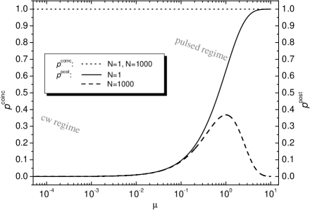
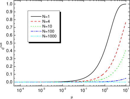
FIG. 2.: (a) Triggering probability $p^{\rm post}$, coincidence-count probability $p^{\rm coinc}$, and (b) multiphoton content $c^{\rm multi}$ for the ideal case: $d=0$, $\eta=1$, and $T_{S}=T_{I}=\Theta=1$. Detection interval $\tau=1$ ns is assumed. The curves showing $p^{\rm coinc}$ for $N=1$ and $N=1000$ coincide.

We now study the influence of real detectors with non-negligible noise and limited quantum efficiency ($\eta<1$, $d>0$, $T_{S}=T_{I}=\Theta=1$). In general, the lower the quantum efficiency $\eta$, the worse the exclusion of multiphoton states in the idler field. Nonzero values of $d$ lead in principle to the occurrence of vacuum state in the idler field.

The triggering probability $p^{\rm post}$ (see Fig. 3a) is now lower than in the previous ideal case owing to losses in the postselection device stemming from limited quantum efficiencies of the detectors. Maximum of the triggering probability $p^{\rm post}$ in case with many detectors is shifted to higher values of the mean number of pairs $\mu$ for the same reason. The coincidence-count probability $p^{\rm coinc}$ approaches unity only in the high-intensity limit. It drops with decreasing mean number of pairs $\mu$. The more the detectors, the faster the decrease. The reason lies in the increased number of ‘false’ triggers in the postselection device due to dark counts of the detectors. This fact is also reflected in the plot of the vacuum probability $p^{\rm vac}$ in Fig. 3b. The use of several detectors brings only a moderate improvement in the exclusion of multiphoton states (see Fig. 3b). The dependence of the Fano factor $F$ on the mean number of pairs $\mu$ is given by the weights of the vacuum and multiphoton contributions. The vacuum contribution prevails for low values of $\mu$, whereas the multiphoton contribution is crucial for high values of $\mu$. Photon number squeezing with $F<0.05$ is achievable for the mean number of pairs $\mu$ in the region $10^{-4}<\mu<10^{-1}$ and for $N<10$ .

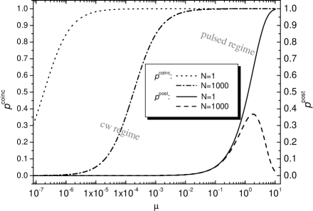
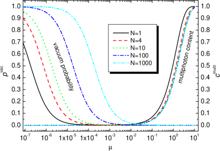
FIG. 3.: (a) Triggering probability $p^{\rm post}$, coincidence-count probability $p^{\rm coinc}$, (b) vacuum probability $p^{\rm vac}$, and multiphoton content $c^{\rm multi}$ for the case with real detectors (values of parameters appropriate for silicon avalanche detectors are used); $d^{dark}=10^{-7}$ (According to Eq. (18), $d^{\rm dark}=\mu^{\rm dark}/(1+\mu^{\rm dark})$, $\mu^{\rm dark}$ being the mean number of dark counts. For $\mu^{\rm dark}\ll 1$, $d^{\rm dark}\approx\mu^{\rm dark}$; $\tilde{\mu}^{\rm dark}=100$ s^-1 and the detection interval $\tau=1$ ns are assumed), $\eta=0.55$, and $T_{S}=T_{I}=\Theta=1$.

Photons in the signal and idler fields are not perfectly entangled in a real experiment, because pairs of photons can be broken as they propagate towards detectors (see Appendix C). Photons that lost their twins then contribute to noise both in the signal and idler beams. As a result, the coincidence-count probability $p^{\rm coinc}$ decreases and almost all advantages of the many-detector device are lost for low coupling coefficients $T_{S}$ and $T_{I}$. The dependencies of vacuum probability $p^{\rm vac}$ and multi-photon content $c^{\rm multi}$ as functions of the mean number of pairs $\mu$ for a typical experiment are plotted in Fig. 4a. The vacuum contribution is now considerable due to triggers by photons that lost their twins. For low $\mu$ this is accented even more by dark counts of the detectors. The exclusion of multiphoton states is very inefficient. The postselection procedure works even worse in the presence of additional noise (see Eq. (13)) caused, e.g., by misalignment of the mode-selecting pinholes or by stray light, as documented by the dash-dot lines in Fig. 4a. Fig. 4b shows the dependence of the Fano factor $F$ on the mean number of pairs $\mu$ under the same conditions. Clearly, the achievable photon-number squeezing is severely limited by the coupling coefficient $\Theta$, $\Theta=T_{S}=T_{I}$ ($F$ reaches values round 0.05 for $\Theta=1$). The destructive influence of the additional noise is also clearly visible.

The crucial role of the coupling coefficient $\Theta$ is documented in Fig. 5 for typical values of the mean number of pairs $\mu$ in the down-conversion experiment pumped by cw and pulsed laser. In the cw regime, good approximations of single-photon Fock states ($F\rightarrow 0$) can be generated in the perfect coupling limit ($\Theta\rightarrow 1$), because the vacuum state probability $p^{\rm vac}$ can be made very small (with low-noise detectors and little additional noise) and the multiphoton content $c^{\rm multi}$ is negligible due to low values of $\mu$. The use of several detectors in the postselection device is not useful; the detectors even increase the total dark-count rate. On the other hand, the use of several detectors yields a significant improvement for higher values of $\Theta$ in the pulsed regime because the exclusion of multiphoton states from the idler field becomes efficient. It is, however, never perfect for a realistic number of detectors. This is the reason why not so good values of photon-number squeezing (low values of $F$) are achievable compared to the cw regime.

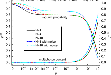
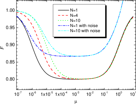
FIG. 4.: (a) Vacuum probability $p^{\rm vac}$, multiphoton content $c^{\rm multi}$, and (b) Fano factor $F$ as functions of the mean number of pairs $\mu$; $T_{S}=T_{I}=\Theta=0.2$, $d^{\rm dark}=10^{-7}$, $\eta=0.55$, $\tau=1$ ns, $\mu_{S}^{\rm res,add}=\mu_{I}^{\rm res,add}=0$ ($\mu_{S}^{\rm res,add}=\mu_{I}^{\rm res,add}=0.04\mu$ for curves denoted as with noise).

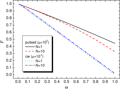
FIG. 5.: Fano factor $F$ as a function of the coupling coefficient $\Theta=T_{S}=T_{I}$ for typical values of the mean number of pairs $\mu$ in cw regime ($\mu=10^{-4}$) and in pulsed regime ($\mu=1$); $d^{\rm dark}=10^{-7}$, $\eta=0.55$, $\tau=1$ ns, and $\mu_{S}^{\rm res,add}=\mu_{I}^{\rm res,add}=0$.

The principle of the postselection device is well illustrated in Figs. 6a,b where the histograms of the photon-number distribution $p(n,\Theta)$ as a function of the coupling coefficient $\Theta=T_{S}=T_{I}$ assuming pulsed pumping are plotted. In the ideal case (Fig. 6a) employing large number of noiseless detectors with the quantum efficiency $\eta=1$, we can see that a perfect elimination of both multiphoton and vacuum contributions is achieved for high values of the coupling coefficient $\Theta$. Using a realistic postselection device, however, the exclusion of multiphoton contributions fails owing to a limited number of detectors and their limited quantum efficiencies. On the other hand an almost perfect exclusion of the vacuum state is still achievable with today’s silicon detectors.

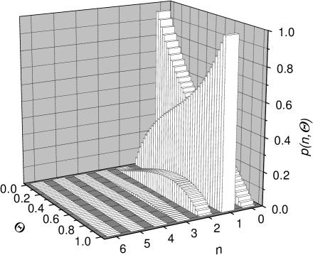
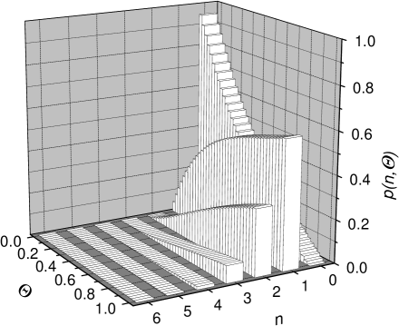
FIG. 6.: Photon number distribution $p(n,\Theta)$ ($n$ denotes the photon number, $\Theta=T_{S}=T_{I}$) of the state obtained in the idler beam if (a) $N=100$ ideal detectors ($d^{\rm dark}=0,\eta=1$) and (b) $N=10$ realistic detectors ($d^{\rm dark}=10^{-7},\eta=0.55$) are used in the postselection device (symmetric $1\times N$ coupler is considered). Pulsed regime is considered ($\mu=1$).

IV Use of the source for QKD

A gap between the ultimate proofs of security of QKD and practical systems exists, because the proofs including most general attacks allowed by quantum mechanics [6, 7] still need to make assumptions that are not implementable in the laboratory and therefore do not yield an instruction how to build a QKD system (one of these assumptions invoked in [6] is the existence of a single-photon source). However, if we slightly weaken our security requirements and limit the eavesdropper to attacks on single particles only (omitting the so-called coherent attacks), there is a proof due to Lütkenhaus that is in correspondence with current experimental techniques [8]. Here the eavesdropper is allowed to use any general quantum-mechanical measurement on single qubits (or ancillas bound to single qubits) including identification and efficient splitting of multiphoton states together with the possibility to store the states until measurement bases are announced in the public discussion.

According to this proof a QKD system may expediently be characterized by the quantity called gain $G$ [8]. Gain $G$ characterizes the fraction of a bit of the key established by the QKD procedure per qubit sent over a quantum channel. Gain $G$ is determined as follows:

$$G=\frac{1}{2}\,p^{\rm post}\,p^{\rm exp}\,\left(1-c^{\rm EC}-c^{\rm PA}\right).$$ (42)

Here $p^{\rm post}$ is the postselection probability of the source ($p^{\rm post}=r^{\rm s}_{I}$ given in Eq. (22) in our model), $p^{\rm exp}$ is the probability of detection at the receiving station of QKD (usually called Bob) and $c^{\rm EC}$ and $c^{\rm PA}$ are error correction and privacy amplification terms, respectively (for details, see [8]). Gain $G$ is closely connected to key generation rate: the higher the gain $G$, the higher the key generation rate.

Taking into account only single-particle attacks, the $c^{\rm PA}$ term can be expressed as [22, 23]:

$$c^{\rm PA}=1-\frac{p^{\rm exp}-p^{\rm multi}}{p^{\rm exp}}\left\{1-\log_{2}\left[1+4\,e\frac{p^{\rm exp}}{p^{\rm exp}-p^{\rm multi}}-4\left(e\frac{p^{\rm exp}}{p^{\rm exp}-p^{\rm multi}}\right)^{2}\right]\right\},$$ (43)

where $e$ is the bit error rate measured at Bob’s station,

$$p^{\rm multi}=1-\sum_{n=0}^{\infty}\left[\left(1-T_{\rm ALICE}\right)^{n}+nT_{\rm ALICE}\left(1-T_{\rm ALICE}\right)^{n-1}\right](\rho_{I}^{mix,s})_{nn}$$

denotes the probability of multiphoton states at the beginning of the transmission line (after passing through Alice’s device with the transmission coefficient $T_{\rm ALICE}$) and $p^{\rm exp}=p^{\rm exp}_{\rm s}+d_{\rm BOB}^{\rm dark}-p^{\rm exp}_{\rm s}d_{\rm BOB}^{\rm dark}$ stands for the expected rate of Bob’s detections. In the latter relation $d_{\rm BOB}^{\rm dark}$ is dark-count rate of Bob’s detector and $p^{\rm exp}_{\rm s}$ means signal rate at Bob’s station. The signal rate $p^{\rm exp}_{\rm s}$ can be expressed as:

$$p_{\rm s}^{\rm exp}=\sum_{j=1}^{\infty}(\rho^{\rm mix,s}_{I})_{jj}\sum_{l=1}^{j}\left(\begin{array}[]{c}j\\ l\end{array}\right)\left(T_{TL}T_{\rm ALICE}\,\eta_{\rm BOB}\right)^{l}\left(1-T_{TL}T_{\rm ALICE}\,\eta_{\rm BOB}\right)^{j-l}.$$ (44)

The symbol $T_{TL}=10^{\left(-\alpha L+l_{\rm BOB}\right)/10}$ denotes the transmission coefficient of the transmission line, $\alpha$ is fiber-attenuation factor, $L$ means fiber length, $l_{\rm BOB}$ denotes losses of Bob’s apparatus, and $\eta_{\rm BOB}$ stands for quantum efficiency of Bob’s detector. The bit error rate $e$ in the absence of an eavesdropper is caused either by physical imperfections (at a rate $c$) or by dark counts of Bob’s detector at the rate 0.5 and we therefore have:

$$e=\frac{c\,p_{\rm s}^{\rm exp}+\frac{1}{2}d^{\rm dark}_{\rm BOB}-\frac{1}{2}c\,p_{\rm s}^{\rm exp}d^{\rm dark}_{\rm BOB}}{p^{\rm exp}}.$$ (45)

The error correction term $c^{\rm EC}$ is expressed by the formula [25]:

$$c^{\rm EC}\approx-1.16\,\left[e\log_{2}e+\left(1-e\right)\log_{2}\left(1-e\right)\right]$$ (46)

valid for $e\leq 0.05$.

Using dim coherent states there is always an optimum value of the source mean photon number $\mu$ (see Fig. 7).

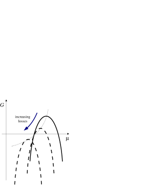
FIG. 7.: A typical curve (solid) characterizing the dependence of the gain $G$ on the mean number of photons $\mu$ of a coherent Poissonian source. Secure QKD is possible if $G\geq 0$. Dashed curves show how the gain $G$ behaves when losses on the transmission line (or length of the fiber) increase. The lower the gain $G$, the lower the optimum mean photon number of the source. If the losses are too high, secure QKD is impossible.

There is a high vacuum content in the signal quantum states for low values of the source mean photon number $\mu$ and so the quantity $c^{\rm EC}$ rapidly grows because physical noises of the detector on Bob’s side become stronger than the signal itself. Each noise count contributes by 50% error rate. On the other hand, the contribution of multiphoton states in the signal field for high values of the source mean photon number $\mu$ requires high values of $c^{\rm PA}$ term which again make the gain $G$ negative at some point. If the gain $G$ is positive for the optimum source mean photon number $\mu$, secure QKD can be performed. There is a maximum allowed amount of losses (or a maximum achievable length of the fiber) for which the required security is still preserved (though at a very low gain). Unfortunately the distances achievable with dim coherent states are rather low, about 8 km using the 800 nm communication window in optical fibers, or about 25 km in the 1550 nm region [8]. Both communication windows have their caveats. While silicon detectors currently used at 800 nm exhibit very low noise (dark-count rates less than 100 s^-1) and high quantum efficiencies ($\eta>0.5$), the losses of the transmission line are very high ($\sim 2.5$ dB km^-1). Just the opposite is available at 1550 nm: transmission-line losses below 0.2 dB km^-1 and detectors with quantum efficiencies below 0.2 and with $10^{4}\div 10^{5}$ dark counts per second.

Lütkenhaus considered an idealized model of the source based on postselection from entangled photon pairs and found out [8] that the communication distance might extend up to 110 km when a local postselection device operating at 800 nm is used and the transmission line is in the low-loss 1550 nm window. This represents an optimum choice with current technology.

We first analyze an idealized postselection device in our model. We thus consider noiseless detectors ($d^{\rm dark}=0$) with unity quantum efficiency ($\eta=1$) and perfect coupling ($T_{S}=T_{I}=\Theta=1$). The idler beam is led from Alice ($T_{\rm ALICE}=0.79$) to Bob’s realistic detector ($\eta_{\rm BOB}=0.18$, $d_{\rm BOB}^{\rm dark}=2\times 10^{-5}$) using 1550 nm transmission line ($\alpha=0.2$ dB km^-1, $c=0.01$). We can see in Fig. 8 that the upper limit of the communication distance extends up to 161 km. This is more than six times the distance achievable with coherent states. This is mainly because the transmitted quantum states contain only a small contribution of the vacuum state. The use of more detectors in the postselection device (this improves the photon-number resolution) does not lead to any further extension of the communication distance. The reason is that the maximum distance is given by the signal-to-noise ratio at Bob’s detector that becomes too low when $p^{\rm exp}_{\rm s}$ drops to the order of $d_{\rm BOB}^{\rm dark}$, i.e. deep down below unity. The multiphoton content $c^{\rm multi}$ in the signal field is negligible in this case. Nevertheless, the improvement of the photon-number resolution leads to an improvement of the gain $G^{\rm opt}$ up to several orders of magnitude (see Fig. 8) and therefore to an improvement of the key generation rate.

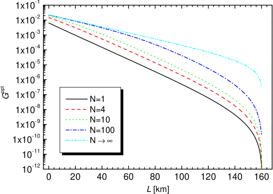
FIG. 8.: Optimum gain $G^{\rm opt}$ of the down-conversion source as a function of the transmission distance $L$ using ideal postselection device ($\eta=1$, $d^{\rm dark}=0$, $T_{S}=T_{I}=\Theta=1$) and realistic transmission line at 1550 nm ($T_{\rm ALICE}=0.79$, $\alpha=0.2$ dB km^-1, $c=0.01$, $\eta_{\rm BOB}=0.18$, $d_{\rm BOB}^{\rm dark}=2\times 10^{-5}$); $\mu^{\rm res,add}_{S}=\mu^{\rm res,add}_{I}=0$. The maximum achievable transmission distance is characterized by the drop of the optimum gain $G^{\rm opt}$.

The dependence of the optimum mean number of pairs $\mu^{\rm opt}$ as a function of the transmission distance $L$ changes significantly if parameters appropriate for a realistic postselection device are considered. If the coupling coefficient $\Theta$ of the photon pairs is set to 0.2 ($\Theta=T_{S}=T_{I}=0.2$, this value is typical for current down-conversion experiments, cf. Appendix C) and parameters of realistic detectors are used ($\eta=0.55$, $d=10^{-7}$), the maximum communication distance drops down to about 120 km (see Fig. 9a). This distance is still significantly better than that achieved with coherent states. The use of more detectors in the postselection device brings, however, no advantage (curves for $N=1,4,10$ almost coincide in Fig. 9a). A closer view (see the inset in Fig. 9a) shows that it causes even a slight drop in the optimum key generation rate for short distances. The reason lies in the fact that the efficiency of the exclusion of multiphoton states is very low due to low values of the coupling coefficient $\Theta$ and the negative influence of detector noise appears to be more significant.

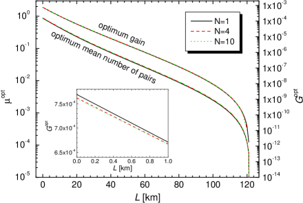
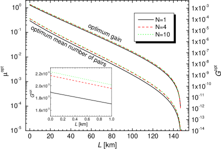
FIG. 9.: Optimum mean number of pairs $\mu^{\rm opt}$ of the down-conversion source and optimum QKD gain $G^{\rm opt}$ in the dependence of the transmission distance $L$ (a) for realistic postselection device at 800 nm ($\eta=0.55$, $d^{\rm dark}=10^{-7}$, $T_{S}=T_{I}=\Theta=0.2$) and realistic transmission line at 1550 nm ($T_{\rm ALICE}=0.79$, $\alpha=0.2$ dB km^-1, $c=0.01$, $\eta_{\rm BOB}=0.18$, $d_{\rm BOB}^{\rm dark}=2\times 10^{-5}$) and (b) for improved postselection device using best current experimental skills ($\eta=0.7$, $d^{\rm dark}=2\times 10^{-8}$, $T_{S}=T_{I}=\Theta=0.6$) and realistic transmission line at 1550 nm ($T_{\rm ALICE}=0.79$, $\alpha=0.2$ dB km^-1, $c=0.01$, $\eta_{\rm BOB}=0.18$, $d_{\rm BOB}^{\rm dark}=2\times 10^{-5}$); $\mu^{\rm res,add}_{S}=\mu^{\rm res,add}_{I}=0$. Curves for $N=1,4,10$ in Fig. 9a) almost coincide. $G^{\rm opt}$ for short distances $L$ are shown in insets.

Increase in the key generation rate is achievable with today’s best technology (see Fig. 9b). Using parameters of a recent down-conversion experiment [28] where a significant improvement of the coupling coefficient $\Theta$ has been achieved, we find the maximum achievable transmission distance to be about 148 km. Moreover, the optimum key generation rate can now be increased employing $N>1$ detectors in the postselection device and is about three times higher than that for the values of parameters used in Fig. 9a.

A crucial role of the coupling coefficient $\Theta$ of photon pairs is illustrated in Fig. 10.

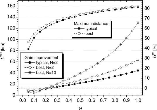
FIG. 10.: Maximum achievable transmission distance $L_{\rm max}$ (rectangles) as a function of the coupling coefficient $\Theta$ ($\Theta=T_{S}=T_{I}$) for realistic postselection device at 800 nm using typical values for current down-conversion experiments (filled symbols) ($\eta=0.55$, $d^{\rm dark}=10^{-7}$, $\mu_{S}^{\rm res,add}=\mu_{I}^{\rm res,add}=0.04\mu$, $N=1$) and best today achievable values of parameters (open symbols) ($\eta=0.7$, $d^{\rm dark}=2\times 10^{-8}$, $\mu_{S}^{\rm res,add}=\mu_{I}^{\rm res,add}=0$, $N=1$). In both cases, a realistic transmission line at 1550 nm is employed ($T_{\rm ALICE}=0.79$, $\alpha=0.2$ dB km^-1, $c=0.01$, $\eta_{\rm BOB}=0.18$, $d_{\rm BOB}^{\rm dark}=2\times 10^{-5}$). The curves with circles show the relative gain improvement $G^{\rm rel}$ reached with the postselection device with $N=2$ detectors and values of parameters typical for current down-conversion experiments (filled circles), with $N=2$ detectors and best today achievable values of parameters (open circles), and with $N=10$ detectors and best today achievable values of parameters (crossed circles) compared to the case with $N=1$ at short communication distances ($L=0$).

If values of $\Theta$ are greater than certain value $\Theta_{\rm min}$ (for our parameters $\Theta_{\rm min}\approx 0.2$) then the better the coupling, the longer the communication distance. Moreover, the better the coupling, the more efficient the resolution of multiphoton states. This then results in the gain improvement provided that more detectors are used. To be more specific, the use of two detectors in a QKD system characterized by typical values of parameters (see Fig. 10) results in the improvement of the relative gain $G^{\rm rel}$ by more than 10 % provided that the coupling coefficient $\Theta$ is greater than $0.7$. Values of the coupling coefficient $\Theta$ have to be greater than $0.55$ in a QKD system characterized by best today available values of parameters (see Fig. 10). The use of more than two detectors in this case results in greater values of relative gain $G^{\rm rel}$, as is documented in Fig. 10 for $N=10$.

We note that the above mentioned expression for the gain $G$ in Eq. (28) can be used for the determination of an optimum combination of elements with given characteristics (transmission coefficents, quantum efficiencies of detectors, noises) in a practical implementation of a quantum key distribution system.

V Conclusions

We have suggested a source of single-photon states using a source of entangled photon pairs (nonlinear crystal with parametric down-conversion) and postselection in one of the entangled beams. Based on an approximate photon-number measurement performed with a $1\times N$ coupler and $N$ detectors in the signal beam, some realizations of the state in the idler field are selected.

An ideal device (perfect alignment of the setup, noiseless detectors with quantum efficiency one) provides nearly single-photon states. Real devices generate states with worse statistics. Dark counts of the detectors and noise coming from decorrelated photons and stray light increase the weight of the vacuum state in the postselected (idler) field. Limited quantum efficiencies of the detectors as well as noise prevent from a perfect exclusion of multiphoton states in the postselected field. However, a field close to a single-photon state may be generated assuming good coupling of photons in the setup and pulsed pumping of the down-conversion process; low-noise detectors have to be used for cw pumping. Such a field is considerably squeezed in photon number (it has sub-Poissonian statistics) and provides a useful source for quantum cryptography.

The suggested source with ideal values of parameters extends the maximum communication distance of QKD about six times (compared to a traditional coherent Poissonian source) up to 160 km. The source with currently achievable values of parameters may be used for the communication distances up to 120 km. Using the best values of parameters available today, the maximum communication distance extends up to 150 km. The maximum communication distance is practically the same for different numbers of detectors in the signal beam. However, the higher the number of detectors in the signal beam, the higher the gain and therefore also the transmission rate. The quality of coupling of the entangled photon pairs is a crucial parameter both for achieving long communication distances and optimum transmission rates. Improvement of the coupling is a challenge for experimentalists.

VI Acknowledgement

This work was supported by the Ministry of Education of the Czech Republic (projects no. LN00A015 and no. 19982003012).

A Detection operator including effects of noise

We assume that the signal field with the density matrix $\hat{\rho}_{S}$ is mixed at the detector with a statistically independent noisy field with the density matrix $\hat{\rho}_{R}$. Detection operator $\hat{P}_{SR}$ describing detection of a photon either from the signal or the noisy field has the form:

$$\hat{P}_{SR} = \sum_{n=1}^{\infty}\left[1-(1-\eta)^{n}\right]|n\rangle_{S}{}_{S}\langle n|\hat{1}_{R}$$ (A2)

$$\mbox{}+\sum_{n=0}^{\infty}(1-\eta)^{n}|n\rangle_{S}{}_{S}\langle n|\sum_{k=1}^{\infty}\left[1-(1-\eta)^{k}\right]|k\rangle_{R}{}_{R}\langle k|,$$

where $|n\rangle_{S}$ ($|k\rangle_{R}$) denotes a Fock state of the signal (noisy) field and $\eta$ stands for the quantum efficiency of the detector.

Detection operator $\hat{P}_{S}$ relevant to the signal field is obtained from the detection operator $\hat{P}_{SR}$ in Eq. (A1) by tracing over the noisy-field space:

$$\hat{P}_{S} = {\rm Tr}_{R}\left\{\hat{P}_{SR}\right\}$$ (A3)

$$= \sum_{n=1}^{\infty}\left[1-(1-\eta)^{n}\right]|n\rangle_{S}{}_{S}\langle n|+d\sum_{n=0}^{\infty}(1-\eta)^{n}|n\rangle_{S}{}_{S}\langle n|.$$ (A4)

The constant $d$ has the form:

$$d=\sum_{k=1}^{\infty}\left[1-(1-\eta)^{k}\right]{}_{R}\langle k|\hat{\rho}_{R}|k\rangle_{R}.$$ (A5)

The relation $0\leq d\leq 1$ follows from Eq. (A3). The higher the mean number of photons in the noisy field, the higher the value of $d$.

If several noise sources are present at the detector, the constant $d$ in Eq. (A2) is defined as follows:

$$d=d_{R1}+(1-d_{R1})d_{R2}+(1-d_{R1})(1-d_{R2})d_{R3}+\ldots,$$ (A6)

where the constants $d_{R1}$, $d_{R2}$, $d_{R3}$, $\ldots$ describe the influence of noisy fields $R_{1}$, $R_{2}$, $R_{3}$, $\ldots$ and are determined according to Eq. (A3).

B Statistics in multimode parametric frequency down-conversion

Expanding the interacting fields into harmonic plane waves, the interaction Hamiltonian $\hat{H}_{\rm int}$ of the process of spontaneous parametric frequency down-conversion can be written in the form [1, 26, 27]:

$$\hat{H}_{\rm int}(t) = C_{\rm int}\int_{-L}^{0}dz\,\sum_{k_{p}}\sum_{k_{s}}\sum_{k_{i}}\chi^{(2)}{\cal E}_{p}^{(+)}(0,\omega_{k_{p}}-\omega^{0}_{p})\hat{a}_{s}^{\dagger}(k_{s})\hat{a}_{i}^{\dagger}(k_{i})$$ (B2)

$$\mbox{}\times\exp\left[i(k_{p}-k_{s}-k_{i})z-i(\omega_{k_{p}}-\omega_{k_{s}}-\omega_{k_{i}})t\right]+\mbox{H.c.}$$

$$= \hat{H}^{(-)}_{\rm int}(t)+\hat{H}^{(+)}_{\rm int}(t).$$ (B3)

where $C_{\rm int}$ is a constant and $\chi^{(2)}$ stands for the second-order susceptibility. The symbol ${\cal E}_{p}^{(+)}(0,\omega_{k_{p}}-\omega^{0}_{p})$ denotes the positive-frequency part of the envelope of the pump-beam electric-field amplitude at the output plane of the crystal; $k_{p}$ stands for the wave vector of a mode in the pump beam and $\omega^{0}_{p}$ means the central frequency of the pump beam. The symbol $\hat{a}_{s}^{\dagger}(k_{s})$ ($\hat{a}_{i}^{\dagger}(k_{i})$) represents the creation operator of the signal (idler) mode with wave vector $k_{s}$ ($k_{i}$) and frequency $\omega_{k_{s}}$ ($\omega_{k_{i}}$). The nonlinear crystal extends from $z=-L$ to $z=0$. The symbol ${\rm H.c.}$ denotes Hermitian conjugate. The operator $\hat{H}^{(-)}_{\rm int}$ ($\hat{H}^{(+)}_{\rm int}$) stands for the part of the interaction Hamiltonian $\hat{H}_{\rm int}$ containing creation (annihilation) operators of modes in the signal and idler fields.

The state of the signal and idler fields at the output plane of the crystal determined by the solution of the Schrödinger equation can be written as follows:

$$|\psi\rangle = \sum_{n=0}^{\infty}|\psi_{n}\rangle,$$ (B4)

$$|\psi_{0}\rangle = |{\rm vac}\rangle,$$ (B5)

$$|\psi_{n}\rangle = \left(-\frac{i}{\hbar}\right)^{n}\int_{-\infty}^{\infty}d\tau_{1}\int_{-\infty}^{\tau_{1}}d\tau_{2}\ldots\int_{-\infty}^{\tau_{n-1}}d\tau_{n}$$ (B7)

$$\mbox{}\times\hat{H}_{\rm int}(\tau_{1})\ldots\hat{H}_{\rm int}(\tau_{n})|{\rm vac}\rangle,\hskip 28.45274ptn=1,2,\ldots.$$

We have assumed that the signal and idler fields are in the vacuum state $|{\rm vac}\rangle$ at the input plane of the crystal.

Assuming that the number of photons in the signal and idler fields is much lower than the number of modes constituting these fields, we may approximately write:

$$|\psi_{n}\rangle = \left(-\frac{i}{\hbar}\right)^{n}\int_{-\infty}^{\infty}d\tau_{1}\int_{-\infty}^{\tau_{1}}d\tau_{2}\ldots\int_{-\infty}^{\tau_{n-1}}d\tau_{n}\hat{H}^{(-)}_{\rm int}(\tau_{1})\ldots\hat{H}^{(-)}_{\rm int}(\tau_{n})|{\rm vac}\rangle$$ (B8)

$$= \left(-\frac{i}{\hbar}\right)^{n}\frac{1}{n!}\left[\int_{-\infty}^{\infty}d\tau\hat{H}^{(-)}_{\rm int}(\tau)\right]^{n}|{\rm vac}\rangle,\hskip 28.45274ptn=1,2,\ldots.$$ (B9)

State $|\psi_{n}\rangle$ then describes the field with exactly $n$ pairs in the signal and idler fields.

Photon statistics in the signal field may be determined from the averages of the normally-ordered operators $\hat{N}^{(n)}_{s}$ for $n=1,2,\ldots$;

$$\hat{N}^{(n)}_{s}(\tau_{1},\ldots,\tau_{n},\tau_{n},\ldots,\tau_{1})=\left[\prod_{j=1}^{n}\hat{E}^{(+)}_{s}(\tau_{j})\right]\left[\prod_{j=1}^{n}\hat{E}^{(-)}_{s}(\tau_{j})\right].$$ (B10)

The symbol $\hat{E}^{(+)}_{s}(\tau)$ ($\hat{E}^{(-)}_{s}(\tau)$) stands for the positive- (negative-) frequency part of the electric-field amplitude of the signal field:

$$\hat{E}^{(+)}_{s}(\tau)=\sum_{k_{s}}e_{s}(k_{s})\hat{a}_{s}(k_{s})\exp(-i\omega_{k_{s}}\tau).$$ (B11)

The symbol $e_{s}(k_{s})$ denotes the normalization amplitude of the mode $k_{s}$.

If the down-converted field is in the state $|\psi_{n}\rangle$ given in Eq. (B3), it holds for $n\geq 1$:

$$\langle\psi_{n}|\hat{N}^{(n)}_{s}(\tau_{1},\ldots,\tau_{n},\tau_{n},\ldots,\tau_{1})|\psi_{n}\rangle={\cal P}\left\{\prod_{j=1}^{n}\langle\psi_{1}|\hat{N}^{(1)}(\tau_{i_{j}},\tau_{j})|\psi_{1}\rangle\right\}.$$ (B12)

The symbol ${\cal P}$ means summation over all permutations of the indices $(i_{1},\ldots,i_{n})$ from the set $(1,\ldots,n)$. Assuming $\langle\psi_{n}|\hat{N}^{(n)}|\psi_{n}\rangle\gg\langle\psi_{k}|\hat{N}^{(n)}|\psi_{k}\rangle$ for $k=n+1,n+2,\ldots$, the relation in Eq. (B6) implies that photon statistics in the signal field is described by the Bose-Einstein distribution.

In order to determine statistics of photon pairs, we define the following “creation operator of photon pairs”:

$$\hat{P}_{\rm pair}(\tau_{s},\tau_{i})=\underline{\hat{E}^{(-)}_{s}(\tau_{s})\hat{E}^{(-)}_{i}(\tau_{i})}.$$ (B13)

Underlining of the operators on the right-hand side of Eq. (B7) means that “only the signal and idler photons created in the same elementary event are considered” (see the expression for $|\psi_{n}\rangle$ in Eq. (B3)).

We may write in the framework of the above used approximation:

$$\langle\psi_{n}|\left[\prod_{j=1}^{n}\hat{P}_{\rm pair}^{\dagger}(\tau_{s_{j}},\tau_{i_{j}})\right]\left[\prod_{j=1}^{n}\hat{P}_{\rm pair}(\tau_{s_{n+1-j}},\tau_{i_{n+1-j}})\right]|\psi_{n}\rangle=$$ (B14)

$$\left[\prod_{j=1}^{n}\langle\psi_{1}|\hat{P}_{\rm pair}^{\dagger}(\tau_{s_{j}},\tau_{i_{j}})|{\rm vac}\rangle\right]\left[\prod_{j=1}^{n}\langle{\rm vac}|\hat{P}_{\rm pair}(\tau_{s_{n+1-j}},\tau_{i_{n+1-j}})|\psi_{1}\rangle\right],$$ (B15)

$$n=1,2,\ldots.$$ (B16)

Assuming that the contribution from the state $|\psi_{n}\rangle$ is much greater that those from the states $|\psi_{k}\rangle$ for $k=n+1,n+2,\ldots$, the relation in Eq. (B8) leads to the conclusion that the statistics of photon pairs is determined by the Poissonian distribution.

C Experimental determination of values of parameters occurring in the model

We give a connection of the model parameters $\mu$, $T_{S}$, $T_{I}$, $\mu_{S}^{\rm res}$, and $\mu_{I}^{\rm res}$ to the measured quantities. An experiment providing detection rates $n_{S}$ and $n_{I}$ at detectors placed in the signal and idler beams and coincidence-count rate $n_{c}$ is assumed.

From the point of view of a real experimental setup, the quantity $\mu$ is determined by the number of photon pairs beyond the nonlinear crystal such that at least one photon of the pair has a nonzero probability of reaching a detector. We further assume that $\mu=kP$, where $P$ is the pump-laser power and $k$ is an unknown constant. We first describe the loss of photons caused by spatial filtering of the signal and idler fields. The loss is caused by the geometric placement of the detectors or pinholes or fiber-coupling optics, whichever is the most limiting. We denote the rate of pairs whose idler (signal) photon is absorbed [the photon cannot reach a detector owing to spatial filtering] by $f_{S}\mu$ ($f_{I}\mu$). The number of entangled pairs in front of the detectors is then given by $(1-f_{S}-f_{I})\mu$. The photons may also be lost owing to absorption and reflection on their paths leading to the detectors (e.g., due to frequency filters). These losses are in general different for ‘pairs’ and ‘singles’. However, we consider them to be the same and represent their influence by beamsplitters with transmission coefficients $t_{S}$ and $t_{I}$ in the signal and idler beams, respectively. This assumption is approximately valid when the losses are only weakly spectrally dependent.

The coincidence-count rate $n_{c}$ is written as:

$$n_{c}=d_{S}d_{I}+\mu t_{S}t_{I}(1-f_{S}-f_{I})\eta_{S}\eta_{I}+O(\mu^{2},d_{S}\mu,d_{I}\mu),$$ (C1)

where $d_{S}$ ($d_{I}$) represents the dark-count rate and $\eta_{S}$ ($\eta_{I}$) is the quantum efficiency of the detector in the signal (idler) beam. This formula is valid, e.g., when cw pumping of the process is applied ($d_{S},d_{I}\ll\mu\ll 1$). Similarly, the detection rates in the signal ($n_{S}$) and idler ($n_{I}$) beams are given as:

$$n_{S} = d_{S}+\mu(1-f_{I})t_{S}\eta_{S}+O(d_{S}\mu),$$ (C2)

$$n_{I} = d_{I}+\mu(1-f_{S})t_{I}\eta_{I}+O(d_{I}\mu).$$ (C3)

Five unknown parameters $\mu$, $f_{S}$, $f_{I}$, $t_{S}$, and $t_{I}$ cannot be uniquely determined from Eqs. (C1) and (C2). In order to simplify the description, we first introduce the quantities $T_{S}$ [$T_{S}=t_{S}(1-f_{I})$] and $T_{I}$ [$T_{I}=t_{I}(1-f_{S})$]. We then replace the coincidence-count rate $n_{c}$ by the quantity $\tilde{n}_{c}$:

$$\tilde{n}_{c}=d_{S}d_{I}+\mu T_{S}T_{I}\eta_{S}\eta_{I}+O(\mu^{2},d_{S}\mu,d_{I}\mu).$$ (C4)

The difference $\tilde{n}_{c}-n_{c}$ equals to $\mu t_{S}t_{I}f_{S}f_{I}\eta_{S}\eta_{I}$ and can be omitted if $f_{S}f_{I}\ll 1$.

The dependencies of $n_{c}$, $n_{S}$, and $n_{I}$ on the pump-laser power $P$ have been measured in the experiment and the constants $b_{c}$, $b_{S}$, and $b_{I}$ characterizing the presumed linear dependencies on the pumping power $P$ have been found. Eqs. (C2) and (C3) then provide equations for the determination of the parameters $k$, $T_{S}$, and $T_{I}$:

$$kT_{S}\eta_{S} = b_{S},$$ (C5)

$$kT_{I}\eta_{I} = b_{I},$$ (C6)

$$kT_{S}T_{I}\eta_{S}\eta_{I} = b_{c}.$$ (C7)

Solving Eqs. (C4), we have:

$$T_{S}=\frac{b_{c}}{\eta_{S}b_{I}},\hskip 14.22636ptT_{I}=\frac{b_{c}}{\eta_{I}b_{S}},\hskip 14.22636ptk=\frac{b_{S}b_{I}}{b_{c}}.$$ (C8)

We cannot determine the values of parameters $t_{S}$, $t_{I}$, $f_{S}$, and $f_{I}$ in our experiment because it does not allow to resolve two above discussed mechanisms causing decorrelation of photons in a pair. However, we can obtain limitations on their values taking into account the relations $0\leq t_{S},t_{I},f_{S},f_{I}\leq 1$:

$$T_{S}\leq t_{S}\leq 1, T_{I}\leq t_{I}\leq 1,$$ (C9)

$$0\leq f_{S}\leq 1-T_{I}, 0\leq f_{I}\leq 1-T_{S}.$$ (C10)

The knowledge of components of the experimental setup may result in stronger limitations on the values of the parameters $t_{S}$ and $t_{I}$ and subsequently also on the values of $f_{S}$ and $f_{I}$.

If the assumption $f_{S}f_{I}\ll 1$ is not valid, correct ratioes of the correlated and decorrelated photons (given by $n_{c}/n_{S}$, $n_{c}/n_{I}$) may be kept by introducing nonzero mean photon numbers of additional noisy fields $\mu^{\rm res,add}_{S}$ and $\mu^{\rm res,add}_{I}$ [see Eqs. (17) and (19); $n_{c}/n_{S}=\tilde{n}_{c}/(n_{S}+\mu^{\rm res,add}_{S})$, $n_{c}/n_{I}=\tilde{n}_{c}/(n_{I}+\mu^{\rm res,add}_{I})$]:

$$\mu_{S}^{\rm res,add} = t_{S}f_{S}f_{I}\frac{1-f_{I}}{1-f_{S}-f_{I}}\mu,$$ (C11)

$$\mu_{I}^{\rm res,add} = t_{I}f_{S}f_{I}\frac{1-f_{S}}{1-f_{S}-f_{I}}\mu.$$ (C12)

As an example, we had $\eta_{S}=0.474$ and $\eta_{I}=0.586$ in our setup and we measured $b_{S}=(5.13\pm 0.05)\times 10^{-5}$ W^-1, $b_{I}=(5.50\pm 0.04)\times 10^{-5}$ W^-1, and $b_{c}=(4.86\pm 0.05)\times 10^{-6}$ W^-1 (detection interval $\tau=1$ ns was used). Using Eqs. (C5), we arrive at:

$$T_{S} = 0.186\pm 0.002,$$ (C13)

$$T_{I} = 0.162\pm 0.002,$$ (C14)

$$k = (5.81\pm 0.09)\times 10^{-4}~{}{\rm W}^{-1}.$$ (C15)

Eqs. (C6) provide the following limitations:

$$0<f_{S}<0.838,\hskip 14.22636pt0<f_{I}<0.814.$$

Using the knowledge of components in the experimental setup, we have $t_{S}<0.25$ and $t_{I}<0.25$ and subsequently

$$0<f_{S}<0.35,\hskip 14.22636pt0<f_{I}<0.25.$$ (C16)

Values of the additional-noise terms are then bounded by the inequalities $0<\mu_{S}^{\rm res,add}<0.041\mu$ and $0<\mu_{I}^{\rm res,add}<0.036\mu$.

D Narrow spectra of the down-converted photons

If the spectra of the down-converted photons are narrow, pairs of photons obey the Bose-Einstein distribution [2] and we have:

$$|c_{n}|^{2}=(1-\nu)\nu^{n},\hskip 28.45274pt\nu=\frac{\mu}{1+\mu},$$ (D1)

where $\mu$ denotes the mean number of photon pairs.

Assuming chaotic noisy fields in the signal and idler beams as given in Eq. (13) and substituting the expression in Eq. (D1) into Eqs. (4) and (12), the diagonal matrix elements of the statistical operator $\hat{\rho}_{I,k}^{\rm mix}$ are determined as follows:

$$(\hat{\rho}_{I,k}^{\rm mix})_{nn} = \frac{(1-\nu^{\rm res}_{I,k})(1-\nu{\cal B})(1-\nu{\cal A}_{k})}{(1-\nu{\cal B})-(1-d_{k})(1-\nu{\cal A}_{k})}$$ (D4)

$$\mbox{}\times\left\{\frac{1}{1-\nu R_{I}{\cal A}_{k}}\,g_{n}\left(\nu^{\rm res}_{I,k},\frac{\nu T_{I}{\cal A}_{k}}{1-\nu R_{I}{\cal A}_{k}}\right)\right.$$

$$\mbox{}\hskip 14.22636pt\left.-\frac{1-d_{k}}{1-\nu R_{I}{\cal B}}\,g_{n}\left(\nu^{\rm res}_{I,k},\frac{\nu T_{I}{\cal B}}{1-\nu R_{I}{\cal B}}\right)\right\},$$

and

$$g_{n}(x,y)=\frac{x^{n+1}-y^{n+1}}{x-y}.$$ (D5)

The expressions for $d^{\rm noise}_{j}$ in Eq. (18) and $\mu^{\rm res}_{I,k}$ in Eq. (19) remain valid also for the coefficients $c_{n}$ given in Eq. (D1). The quantity $r_{I,k}$ is given according to the relation:

$$r_{I,k}=\left[\prod_{l=1,\ldots,N;l\neq k}(1-d_{l})\right]\frac{1-\nu}{1-\nu{\cal A}_{k}}-\left[\prod_{l=1}^{N}(1-d_{l})\right]\frac{1-\nu}{1-\nu{\cal B}}.$$ (D6)

Assuming a symmetric $1\times N$ coupler (described in Eq. (20)) and detection of a photon at an arbitrary detector, we get:

$$(\hat{\rho}_{I}^{\rm mix,s})_{nn} = \frac{(1-\nu^{\rm res}_{I})(1-\nu{\cal B})(1-\nu{\cal A})}{(1-\nu{\cal B})-(1-d)(1-\nu{\cal A})}$$ (D9)

$$\mbox{}\times\left\{\frac{1}{1-\nu R_{I}{\cal A}}\,g_{n}\left(\nu^{\rm res}_{I},\frac{\nu T_{I}{\cal A}}{1-\nu R_{I}{\cal A}}\right)\right.$$

$$\mbox{}\hskip 14.22636pt\left.-\frac{1-d}{1-\nu R_{I}{\cal B}}\,g_{n}\left(\nu^{\rm res}_{I},\frac{\nu T_{I}{\cal B}}{1-\nu R_{I}{\cal B}}\right)\right\},$$

and

$$r_{I}=(1-d)^{N-1}\frac{1-\nu}{1-\nu{\cal A}}-(1-d)^{N}\frac{1-\nu}{1-\nu{\cal B}}.$$ (D10)

REFERENCES

• [1] L. Mandel and E. Wolf, Optical Coherence and Quantum Optics (Cambridge University Press, Cambridge, 1995), chap. 22.4.
• [2] D. F. Walls and G. J. Milburn, Quantum Optics (Springer, Berlin, 1995), chap. 5.
• [3] J. Peřina, Z. Hradil, and B. Jurčo, Quantum Optics and Fundamentals of Physics (Kluwer, Dordrecht, 1994), chap. 8.
• [4] A. K. Ekert, Phys. Rev. Lett. 67, 661 (1991).
• [5] For a review on QKD, see, e.g., D. Bruß, N. Lütkenhaus, Quantum key distribution: from Principles to Practicalities, in: Applicable Algebra in Engineering, Communication and Computing, vol. 10 (Springer, Berlin, 2000), p. 383. Also quant-ph/9901061.
• [6] D. Mayers, Unconditional security in quantum cryptography, in Advances in Cryptology - Proc. Crypto ’96 (Springer, Berlin, 1996), p. 343. Also quant-ph/9802024v4.
• [7] H.-K. Lo and H. F. Chau, Science 283, 2050 (1999). Also quant-ph/9803006.
• [8] N. Lütkenhaus, Phys. Rev. A 61, 052304 (2000).
• [9] W. Tittel, J. Brendel, H. Zbinden, and N. Gisin, Phys. Rev. Lett. 84, 4737 (2000).
• [10] T. Jennewein, Ch. Simon, G. Weihs, H. Weinfurter, and A. Zeilinger, Phys. Rev. Lett. 84, 4729 (2000).
• [11] A. V. Sergienko, M. Atatüre, Z. Walton, G. Jaeger, B. E. A. Saleh, and M. C. Teich, Phys. Rev. A 60, R2622 (2000).
• [12] G. Ribordy, J. Brendel, J.-D. Gautier, N. Gisin, and H. Zbinden, Phys. Rev. A 63, 012309 (2001).
• [13] D. S. Naik, C. G. Peterson, A. G. White, A. J. Berglund, and P. G. Kwiat, Phys. Rev. Lett. 84, 4733 (2000).
• [14] G. Brassard, N. Lütkenhaus, T. Mor, and B. C. Sanders, Phys. Rev. Lett. 85, 1330 (2000).
• [15] O. Haderka and J. Peřina, Jr., Approximations of single-photon states by postselection from correlated pairs, Proc. NATO ARW on Decoherence and its Implications in Quantum Computation and Information Transfer, (Mykonos, Greece, 2000), in print.
• [16] P. Törmä, T. Kiss, I. Jex, and H. Paul, Jemná mechanika a optika 11-12, 338 (1996).
• [17] S. Takeuchi, J. Kim, Y. Yamamoto, and H. H. Hogue, Appl. Phys. Lett. 74, 1063 (1999); J. Kim, O. Benson, H. Kan, and Y. Yamamoto, Nature 397, 500 (1999).
• [18] P. Kok and S. L. Braunstein, Phys. Rev. A 63, 033812 (2001).
• [19] O. Haderka and J. Peřina, Jr., Photon source for quantum cryptography using postselecion from entangled quantum states, SPIE, (Velké Losiny, Czech Republic, 2000), in print.
• [20] R. A. Campos, B. E. A. Saleh, and M. C. Teich, Phys. Rev. A 40, 1371 (1989).
• [21] J. Peřina, Quantum Statistics of Linear and Nonlinear Optical Phenomena (Kluwer, Dordrecht, 1991), 2nd edition.
• [22] C. A. Fuchs, N. Gisin, R. B. Griffiths, C.-S. Niu, and A. Peres, Phys. Rev. A 56, 1163 (1997).
• [23] N. Lütkenhaus, Phys. Rev. A 59, 3301 (1999).
• [24] W. T. Buttler, R. J. Hughes, S. K. Lamoreaux, G. L. Morgan, J. E. Nordholt, and C. G. Peterson, Phys. Rev. Lett. 84, 5652 (2000).
• [25] G. Brassard and L. Salvail, Advances in Cryptology - Proc. Eurocrypt ’93, Lecture Notes in Computer Science, vol. 765 (Springer, Berlin, 1994), p. 410.
• [26] J. Peřina, Jr., A. V. Sergienko, B. M. Jost, B. E. A. Saleh, and M. C. Teich, Phys. Rev. A 59, 2359 (1999).
• [27] J. Peřina, Jr., Eur. Phys. J. D 7, 235 (1999).
• [28] Ch. Kurtsiefer, M. Oberparleiter, and H. Weinfurter, quant-ph/0101074.