Optical mode characterization of single photons prepared via conditional measurements on a biphoton state

Abstract

A detailed theoretical analysis of the spatiotemporal mode of a single photon prepared via conditional measurements on a photon pair generated in the process of parametric down-conversion is presented. The maximum efficiency of coupling the photon into a transform-limited classical optical mode is calculated and ways for its optimization are determined. An experimentally feasible technique of generating the optimally matching classical mode is proposed. The theory is applied to a recent experiment on pulsed homodyne tomography of the single-photon Fock state (A. I. Lvovsky et al., Phys Rev. Lett. 87, 050402 (2001)).

PACS numbers: 42.50.Dv Nonclassical field states; squeezed, antibunched, and sub-Poissonian states; operational definitions of the phase of the field; phase measurements; 42.50.Ar Photon statistics and coherence theory; 03.65.Ud Entanglement and quantum nonlocality

I Introduction.

Quantum states containing a definite number of energy quanta (Fock states) play a key role in quantum optics. They constitute the essence of the quantum nature of light and are indispensable in the theoretical description of a wide range of optical phenomena. Fock states also play a major role in more applied aspects of quantum optics, such as the rapidly developing fields of quantum communication and information. Of particular importance is the application of Fock states in quantum cryptography which would result in a significant increase in capacity and security of communication channels [1]. Superpositions of the vacuum and the single-photon state in a certain optical mode can also be used to implement a qubit. Such an application of the Fock state has been discussed in a recent proposal on efficient linear quantum computation [2].

Despite their importance, pure number states are extremely rare in nature and their synthesis in a laboratory constitutes a rather involved task. In recent years significant efforts have been made towards developing a “photon pistol” — a technology of emitting a single photon into a well-defined traveling spatiotemporal mode upon the onset of a classical trigger. A number of approaches are being tried [3], but none has fully resolved this problem so far. In these circumstances an important alternative is offered by the technique of preparing single photons by conditional measurements on a biphoton state born in the process of parametric down-conversion (PDC) (Fig. 1). In PDC, a “pump” photon propagating through a nonlinear medium may spontaneously annihilate to produce two photons of lower energy in the form of a highly entangled quantum state known as $biphoton$. The two generated photons are separated into two emission channels according to their propagation direction, wavelength and/or polarization. Detection of a photon in one of the emission channels (labeled $trigger$) causes the non-local photon pair to collapse projecting the quantum state in the remaining ($signal$) channel into a single-photon state. Proposed and tested experimentally in 1986 by Hong and Mandel [4] as well as Grangier, Roger and Aspect [5], this technique has become a workhorse for many quantum optics experiments [6].

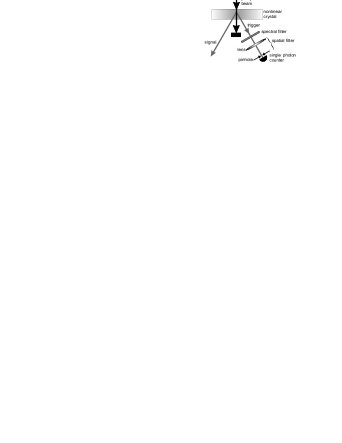
FIG. 1.: Preparation of single photons by conditional measurements on a biphoton state.

Using the conditionally prepared photon (CPP) for practical purposes, such as communication, storage, quantum information processing or synthesis of more complex quantum states, requires the photon to be produced in a well-defined, transform-limited optical mode. While there exists extensive theoretical and experimental research on biphotons and associated quantum effects [7, 8, 9, 10], very little work has been done to analyze the CPP as a “final product”, i.e. in a way that would reveal its quantum state and provide ways for its optimization.

In 1997 Ou presented a qualitative theoretical investigation of the temporal mode of the CPP in application to homodyne tomography [11]. He has shown that in order to prepare the photon in a transform limited temporal mode that could be matched to the local oscillator beam, one has to use a spectral filter in the trigger channel which is much narrower than the linewidth of the pump pulse. In a more recent paper, Grosshans and Grangier considered a similar experiment and quantified the fidelity of mode matching in terms of the efficiency of the tomography measurement [12]. This efficiency was calculated using specific assumptions about the local oscillator mode and a simplified model of the spectral filter has been used. Very recently, the Fock state tomography has been demonstrated experimentally [13], but no theoretical discussion regarding the above matters has been presented.

In this paper we perform a detailed theoretical analysis of the spatiotemporal mode of the CPP using very general assumptions about the spatial and spectral filter in the trigger channel. We calculate the distribution of the CPP state over plane wave modes and discuss ways of its optimal mode matching to a transform-limited classical wave. We determine the theoretical limits imposed on the mode matching parameter and propose a method of constructing a classical field that would match the CPP mode optimally.

II The conditionally prepared single photon

We start with a general calculation of the quantum state of a single photon state prepared by a conditional measurement on a pulsed PDC biphoton state. We restrict our consideration to the pulsed regime. A continuous-wave pump, although highly efficient in generating biphotons [14], does not yield transform-limited CPPs as we demonstrate below. In all calculations in this paper, we neglect polarization entanglement (polarization is assumed to be well-defined in both PDC channels) and refraction inside the crystal.

The interaction Hamiltonian of parametric down-conversion is given by [15]

$$\hat{V} (t)$$ (2)

$$=\alpha\int\tilde{K}({\mathbf{r}})\tilde{E}_{t}^{(-)}({\mathbf{r}},t)\tilde{E}_{s}^{(-)}({\mathbf{r}},t)\tilde{E}_{p}^{(+)}({\mathbf{r}},t)d^{3}r\,+\text{H.c.},$$

where $\alpha$ is proportional to the second order nonlinear susceptibility and is assumed frequency independent, $\tilde{K}({\mathbf{r}})$ describes the nonlinear crystal volume and is one inside and zero outside the crystal. We treat the fields in the signal ($s$) and trigger ($t$) channels as quantum operators, with their positive-frequency components given by

$$\hat{\tilde{E}}_{s,t}^{(+)}({\mathbf{r}},t)=\int e^{-i({\mathbf{k}}_{s,t}\cdot{\mathbf{r}}-\omega_{s,t}t)}\hat{a}_{{\mathbf{k}}_{s,t},\omega_{s,t}}d^{3}k_{s,t}\,d\omega_{s,t};$$ (3)

the coherent pump field is treated classically:

$$\tilde{E}_{p}^{(+)}({\mathbf{r}},t)=\int E_{p}^{(+)}({\mathbf{k}}_{p},\omega_{p})e^{i({\mathbf{k}}_{p}\cdot{\mathbf{r}}-\omega_{p}t)}d^{3}k_{p}\,d\omega_{p}\,.$$ (4)

For all fields, quantum or classical, the Hermitian electric field observable is written as $\tilde{E}_{p}({\mathbf{r}},t)=\tilde{E}_{p}^{(+)}({\mathbf{r}},t)+\tilde{E}_{p}^{(-)}({\mathbf{r}},t)$, with $\tilde{E}_{p}^{(-)}({\mathbf{r}},t)=(\tilde{E}_{p}^{(+)}({\mathbf{r}},t))^{\dagger}$.

Assuming the signal and trigger modes to be initially in the vacuum state and restricting the consideration to the first order perturbation theory, we write the resulting biphoton state as

$${\left|B\right\rangle}={\left|0\right\rangle}_{s}{\left|0\right\rangle}_{t}-i\int_{-\infty}^{\infty}\hat{V}(t)\,dt.$$ (5)

Performing the integration we obtain:

$${\left|B\right\rangle} = {\left|0\right\rangle}_{s}{\left|0\right\rangle}_{t}-i\int d^{3}k_{s}\,d\omega_{s}\,d^{3}k_{t}\,d\omega_{t}$$ (7)

$$\times\,\Psi({\mathbf{k}}_{s},\omega_{s},{\mathbf{k}}_{t},\omega_{t}){\left|1_{{\mathbf{k}}_{s},\omega_{s}}\right\rangle}_{s}{\left|1_{{\mathbf{k}}_{t},\omega_{t}}\right\rangle}_{t},$$

with

$$\Psi({\mathbf{k}}_{s},\omega_{s}, {\mathbf{k}}_{t} ,\omega_{t})$$ (8)

$$= \alpha\int E_{p}^{(+)}({\mathbf{k}}_{p},\omega_{s}+\omega_{t})K(\Delta{\mathbf{k}})d^{3}k_{p}.$$ (9)

Here $K({\mathbf{k}})$ is the Fourier transform of $\tilde{K}({\mathbf{r}})$ and the ${\mathbf{k}}$-vector mismatch is $\Delta{\mathbf{k}}={\mathbf{k}}_{p}-{\mathbf{k}}_{s}-{\mathbf{k}}_{t}$.

The trigger photon is then selected by spatial and frequency filters and is detected by a single-photon counter. Conditioned on the detection event the non-local biphoton state collapses into a single photon state in the signal mode. The properties of this mode are determined by the optical mode of the pump photon and the spatial and spectral filtering in the trigger channel:

$$\hat{\rho}_{s}=\text{Tr}_{t}(\hat{\rho}_{t}{\left|B\right\rangle}{\left\langle B\right|}),$$ (10)

where the trace is taken over the trigger states and $\hat{\rho}_{t}$ denotes the state ensemble selected by the filters:

$$\hat{\rho}_{t}=\int T({\mathbf{k}}_{t},\omega_{t}){\left|1_{{\mathbf{k}}_{t},\omega_{t}}\right\rangle}_{t}{\left\langle 1_{{\mathbf{k}}_{t},\omega_{t}}\right|}_{t}\,d^{3}k_{t}\,d\omega_{t}\,$$ (11)

with $T({\mathbf{k}},\omega)$ being the spatiotemporal transmission function of the filters.

The expression (11) is different from the one used by Grosshans and Grangier [12] who associated a monochromator of width $\delta\omega$ with a pure state of the form ${\left|\psi_{t}\right\rangle}=\int_{-\delta\omega/2}^{\delta\omega/2}{\left|1_{\omega_{0}+\delta\omega}\right\rangle}\,d\delta\omega$. A spectral filter does not distinguish relative phases of different frequency components of the transmitted ensemble; we have therefore assumed all non-diagonal elements of the trigger density matrix to vanish.

An explicit calculation of the quantum state (10) of the photon in the signal channel yields

$$\hat{\rho}_{s}= \int d^{3}k_{s}d\omega_{s}d^{3}k_{s}^{\prime}d\omega_{s}^{\prime}$$ (13)

$$\Phi({\mathbf{k}}_{s},\omega_{s},{\mathbf{k}}_{s}^{\prime},\omega_{s}^{\prime}){\left|1_{{\mathbf{k}}_{s}^{\prime},\omega_{s}^{\prime}}\right\rangle}_{s}{\left\langle 1_{{\mathbf{k}}_{s},\omega_{s}}\right|}_{s},$$

where

$$\Phi({\mathbf{k}}_{s},\omega_{s},{\mathbf{k}}_{s}^{\prime},\omega_{s}^{\prime}) = |\alpha|^{2}\int d^{3}k_{t}\,d\omega_{t}\,d^{3}k_{p}\,\,d^{3}k_{p}^{\prime}\,$$ (16)

$$\times\,E_{p}^{(-)}({\mathbf{k}}_{p},\omega_{s}+\omega_{t})E_{p}^{(+)}({\mathbf{k}}_{p}^{\prime},\omega_{s}^{\prime}+\omega_{t})$$

$$\times\,T({\mathbf{k}}_{t},\omega_{t})K^{*}(\Delta{\mathbf{k}})K(\Delta{\mathbf{k}}^{\prime}),$$

with $\Delta{\mathbf{k}}$ as above and $\Delta{\mathbf{k}}^{\prime}={\mathbf{k}}_{p}^{\prime}-{\mathbf{k}}_{s}^{\prime}-{\mathbf{k}}_{t}$.

III The measure of mode matching

To discuss the main question of this paper — how to match a classical wave to the spatiotemporal mode of the CPP — we first need to introduce a quantitative measure of mode matching. We characterize both modes by their correlation functions, defined as $\Gamma({\mathbf{k}},\omega,{\mathbf{k}}^{\prime},\omega^{\prime})={<\hat{E}{(-)}({\mathbf{k}},\omega)\hat{E}{(+)}({\mathbf{k}}^{\prime},\omega^{\prime})>}$, with the averaging done in the statistical sense for the classical field and in the quantum-mechanical sense for the single-photon field. For the latter, using $\hat{E}^{(+)}({\mathbf{k}},\omega)\propto\hat{a}_{{\mathbf{k}},\omega}$ and applying Eq. (13), we find:

$$\Gamma({\mathbf{k}},\omega,{\mathbf{k}}^{\prime},\omega^{\prime})={\rm Tr}(\hat{\rho}_{s}\,\hat{a}^{\dagger}_{{\mathbf{k}},\omega}\,\hat{a}_{{\mathbf{k}}^{\prime},\omega^{\prime}})=\Phi({\mathbf{k}},\omega,{\mathbf{k}}^{\prime},\omega^{\prime}),$$ (17)

i.e. the field correlation function coincides with the density matrix of the single photon state.

It is natural to define the degree of mode matching between two waves characterized by their correlation functions $\Gamma_{1,2}({\mathbf{k}},\omega,{\mathbf{k}}^{\prime},\omega^{\prime})$ as follows:

$$M=\frac{\int d^{3}k\,d\omega\,d^{3}k^{\prime}\,d\omega^{\prime}\,\Gamma_{1}({\mathbf{k}},\omega,{\mathbf{k}}^{\prime},\omega^{\prime})\Gamma_{2}^{*}({\mathbf{k}},\omega,{\mathbf{k}}^{\prime},\omega^{\prime})}{\int d^{3}k\,d\omega\,\Gamma_{1}({\mathbf{k}},\omega,{\mathbf{k}},\omega)\int d^{3}k\,d\omega\,\Gamma_{2}({\mathbf{k}},\omega,{\mathbf{k}},\omega)}.$$ (18)

If both waves $\Gamma_{1}$ and $\Gamma_{2}$ are classical, the mode matching parameter is equal to the square of the visibility of the pattern that would be observed if the two modes were caused to interfere. If both waves are single photons, the value of $M$ is the probability of the quantum overlap ${\rm Tr}(\hat{\rho}_{1}\hat{\rho}_{2})$ between the two states. We are most interested in the third case, when one of the $\Gamma$’s represents a CPP, and the other a matching classical wave, and adopt the above expression as the measure of mode matching. Grosshans and Grangier [12] have shown that the expression (18) determines the quantum efficiency in a homodyne tomography measurement of the single-photon Fock state in which the matching classical wave serves as a local oscillator.

Suppose that a single photon is prepared in a certain state $\hat{\rho}_{s}$ and our task is to pick the classical wave that would match the mode of the single photon optimally. As the former is generally not a pure quantum state, no choice of the classical mode can guarantee perfect mode matching. To determine the maximum level of $M$ that can be achieved, we introduce the purity parameter of an optical mode,

$$P=\frac{\int d^{3}k\,d\omega\,d^{3}k^{\prime}\,d\omega^{\prime}\,\Gamma({\mathbf{k}},\omega,{\mathbf{k}}^{\prime},\omega^{\prime})\Gamma^{*}({\mathbf{k}},\omega,{\mathbf{k}}^{\prime},\omega^{\prime})}{(\int d^{3}k\,d\omega\,\Gamma({\mathbf{k}},\omega,{\mathbf{k}},\omega))^{2}},$$ (19)

which is equal to unity for coherent optical modes and vanishes for incoherent ones. For the single-photon states of the form (13), the above quantity can be written in the form of a well-known quantum state purity parameter

$$P={\text{Tr}}(\hat{\rho}_{s}^{2}),$$ (20)

which reaches one for pure quantum states and approaches zero for density matrices with no non-diagonal elements.

It then follows from the Cauchy-Schwartz inequality that for any two optical modes 1 and 2

$$M^{2}\leq P_{1}\,P_{2}.$$ (21)

If mode 1 is a CPP, the right-hand side of the above inequality is maximized if the matching classical mode 2 is a coherent wave, i.e. $P_{1}=1$. In this case,

$$M\leq\sqrt{P_{1}},$$ (22)

which establishes an unconditional theoretical limit to the degree to which a classical wave can be matched to a given single-photon mode (13).

IV Modeling the single photon mode with a classical wave

Our next task is to design a classical wave that matches the CPP mode optimally. Apart from its theoretical aspect, this problem constitutes a substantial challenge in the experimental practice. The traditional procedure of matching two classical modes with each other — by observing interference fringes and optimizing their visibility — is clearly not applicable to the situation when one of the modes is a single photon. There is no laser beam to mode match to. The only information available to the experimentalist is the remote location and width of the trigger filter and the parameters of the pump. Although the spatial location of the CPP can be approximately determined by detecting coincidences between the photon count events in the signal and trigger [8], optimizing the mode matching requires adjustment of a much larger set of degrees of freedom, such as the beam direction, divergence, spatial and temporal width, optical delay, etc. Reliable adjustment of these parameters cannot be achieved through a sole optimization of the coincidence rate.

Fortunately, the CPP mode can be modeled with a classical wave generated in the following way. Suppose an alignment beam is inserted into the trigger channel so that it overlaps spatially and temporally with the pump beam inside the crystal and passes through the optical filters (Fig. 2 (a)). Nonlinear interaction of such an alignment beam with the pump wave will produce difference frequency generation (DFG) into a spatiotemporal mode similar to that of the CPP.

To show this, we write for the nonlinear polarization inside the crystal

$$\tilde{P}_{\rm DFG}({\mathbf{r}},t)\propto\tilde{E}_{A}({\mathbf{r}},t)\tilde{E}_{p}({\mathbf{r}},t).$$ (23)

Here $\tilde{E}_{p}({\mathbf{r}},t)$ and $\tilde{E}_{A}({\mathbf{r}},t)$ are the electric fields of the pump and alignment beams, respectively. The nonlinear polarization gives rise to the DFG field which is obtained from Eq. (23) via a Fourier transform which is restricted to the crystal volume:

$$E^{(+)}_{\rm DFG} ({\mathbf{k}}_{s},\omega_{s})=\beta^{\prime}\,\delta(k_{s}-\omega_{s}/c)\int d^{3}k_{A}\,d\omega_{A}\,d^{3}k_{p}$$ (24)

$$\times E_{A}^{(-)}({\mathbf{k}}_{A},\omega_{A})\,E_{p}^{(+)}({\mathbf{k}}_{p},\omega_{s}+\omega_{A})K(\Delta{\mathbf{k}}).$$ (25)

The proportionality coefficient $\beta$ represents the nonlinearity of the medium. If the alignment field is partially incoherent and is characterized by a correlation function $\Gamma_{A}({\mathbf{k}}_{A},\omega_{A},{\mathbf{k}}_{A}^{\prime},\omega_{A}^{\prime})$, the above equation generalizes to

$$\Gamma_{\rm DFG}({\mathbf{k}}_{s},\omega_{s}, {\mathbf{k}}_{s}^{\prime},\omega_{s}^{\prime})=|\beta^{\prime}|^{2}\,\delta(k_{s}-\omega_{s}/c)\,\delta(k^{\prime}_{s}-\omega^{\prime}_{s}/c)$$ (29)

$$\times\int d^{3}k_{A}\,d\omega_{A}\,d^{3}k_{A}^{\prime}\,d\omega_{A}^{\prime}\,d^{3}k_{p}\,d^{3}k_{p}^{\prime}$$

$$\times\,E_{p}^{(-)}({\mathbf{k}}_{p},\omega_{s}+\omega_{A})E_{p}^{(+)}({\mathbf{k}}_{p}^{\prime},\omega_{s}^{\prime}+\omega_{A}^{\prime})$$

$$\times\,\Gamma_{A}^{*}({\mathbf{k}}_{A},\omega_{A},{\mathbf{k}}_{A}^{\prime},\omega_{A}^{\prime})K^{*}(\Delta{\mathbf{k}})K(\Delta{\mathbf{k}}^{\prime}).$$

We immediately notice that the expressions for the optical mode of the CPP photon (16) and of the DFG pulse (29) are very similar. This similarity can be interpreted in the framework of D. N. Klyshko’s concept of advanced waves [17]. Suppose the single photon detector is replaced by an incoherent source (an “incandescent bulb”) continuously emitting omnidirectional incoherent light into a wide spectral range backwards in time. This completely incoherent light is characterized by the correlation function $\Gamma_{0}({\mathbf{k}}^{\prime},\omega^{\prime},{\mathbf{k}},\omega)=\delta^{(3)}({\mathbf{k}}^{\prime}-{\mathbf{k}})\,\delta(\omega^{\prime}-\omega)$ which, upon passing through the spatial and spectral filters, transforms into

$$\Gamma_{t}({\mathbf{k}}^{\prime},\omega^{\prime},{\mathbf{k}},\omega)=T({\mathbf{k}},\omega)\,\delta^{(3)}({\mathbf{k}}^{\prime}-{\mathbf{k}})\,\delta(\omega^{\prime}-\omega).$$ (30)

The advanced wave then enters the nonlinear crystal and interacts with the pump wave whenever and wherever it is present in the crystal. The nonlinear interaction of Klyshko’s advanced wave with the pump pulse produces a pulse of DFG emission into the signal channel (Fig. 2(b)). Substituting the correlation function (30) of the advanced wave into Eq. (29) as $\Gamma_{A}$ we find that the correlation function $\Gamma_{\rm DFG}({\mathbf{k}}_{s},\omega_{s},{\mathbf{k}}_{s}^{\prime},\omega_{s}^{\prime})$ of the DFG pulse generated through the nonlinear interaction of the advanced wave and the pump pulse is identical to the density matrix $\Phi({\mathbf{k}}_{s},\omega_{s},{\mathbf{k}}_{s}^{\prime},\omega_{s}^{\prime})$ of the single photon prepared via conditional measurements on a biphoton performed in the same optical arrangement.

This identity can be easily generalized to optical filters of random configuration, more complex than a combination of spatial and spectral filters described by Eqs. (11) and (30). Its applicability is also independent from other features of the experimental setup, such as the type of PDC, properties of the pump beam, geometry of the crystal, walk-off and group velocity dispersion effects, etc. and appears to be very general. The only restriction that has to be taken into account is the first order perturbation theory that implies that the probability of generating two or more biphotons at a time is negligible.

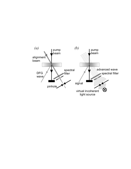
FIG. 2.: (a) Nonlinear interaction of the alignment beam with the pump pulse generates DFG emission; (b) Interaction of Klyshko’s advanced wave with the pump generates a DFG mode that mimics that of the CPP.

By varying the configuration of the filter in the trigger channel one has a degree of freedom in forming the CPP mode with required spatiotemporal properties. This possibility can be considered as an example of remote state preparation in the sense discussed by Bennett et al. [18]. The original biphoton state is highly entangled in the frequency-momentum space and this entanglement plays an essential role in generating the Fock state. The signal mode does not exist unless and until the trigger photon passes through the filters and is registered. A detection event results in a non-local preparation of a single photon in an optical mode whose characteristics are determined by the way in which the measurement in the trigger channel is performed.

V Mode matching: an explicit calculation

A Frequency-momentum representation

We have thus designed an experimentally plausible way of generating a classical wave whose mode models that of the CPP. Although the advanced (i.e. propagating backwards in time) wave is a purely imaginary object, it can be simulated in a laboratory by a coherent laser beam — the alignment wave. As we demonstrate in this section, the proper choice of the latter allows the level of mode matching to reach its theoretical limit set by Eq. (22). To simplify our calculations, we make the following assumptions.

1. Parametric down-conversion occurs in a collinear type II configuration. The signal and trigger channels are then separated according to their polarization. Collinearity of the pump, signal and trigger fields allows to use the same reference frame for all three waves.

2. A simple combination of spatial and spectral filters is used in the trigger channel, so Eqs. (11) and (30) are valid.

3. The crystal volume is much larger than the spatial extent of the pump pulse inside the crystal. This allows us to approximate

$$V(\Delta{\mathbf{k}})\approx\delta^{(3)}(\Delta{\mathbf{k}})$$ (31)

and Eqs. (16) and (29) simplify accordingly.

4. The pump ($p$) and alignment ($A$) fields are collimated inside the crystal and are assumed to be of Gaussian shape:

$$E_{p,A}^{(+)}({\mathbf{k}},\omega)=E_{p,A}^{0}\exp\left(-\frac{{\mathbf{k}}_{\bot}^{2}}{\kappa_{p,A}^{2}}-\frac{(\omega-\omega_{p,A}^{0})^{2}}{\sigma_{p,A}^{2}}\right),$$ (32)

where $\omega_{p,A}^{0}$ are the central frequencies of the two waves, $\sigma_{p,A}$ are their linewidths and $\kappa_{p,A}$ are the beam widths in the momentum space. A similar assumption is made for the transmission of the trigger filter:

$$T({\mathbf{k}},\omega)=T_{0}\exp\left(-\frac{{\mathbf{k}}_{\bot}^{2}}{\kappa_{t}^{2}}-\frac{(\omega-\omega_{t}^{0})^{2}}{\sigma_{t}^{2}}\right).$$ (33)

5. The center frequency of the alignment field coincides with the transmission maximum of the spectral filter, i.e. $\omega_{A}^{0}=\omega_{t}^{0}$ and its direction is collinear with the transmission maximum of the spatial filter.

6. There is no beam walkoff nor group velocity dispersion.

Under these assumptions, the calculation of the mode matching and the purity parameter substantially simplifies as the temporal variables separate from the two spatial ones and the resulting values of $M$ and $P$ are products of three similar expressions for the temporal and spatial (in two orthogonal dimensions) mode matching and mode purity parameters. In this subsection, we restrict ourselves to the temporal domain keeping in mind that the calculation in the spatial domain would be completely analogous.

The density matrix of the CPP mode are determined using Eq. (16):

$$\Phi(\omega,\omega^{\prime})$$ (34)

$$\,=\Gamma_{s}^{0}\exp\biggl{(}-\frac{(\omega-\omega_{s}^{0})^{2}+(\omega^{\prime}-\omega_{s}^{0})^{2}}{(\sigma_{p}^{2}+2\sigma_{t}^{2})}-\frac{\sigma_{t}^{2}(\omega-\omega^{\prime})^{2}}{\sigma_{p}^{2}(\sigma_{p}^{2}+2\sigma_{t}^{2})}\biggl{)}.$$ (35)

where $\Gamma_{0}^{s}$ is a constant factor and $\omega_{s}^{0}=\omega_{p}^{0}-\omega_{t}^{0}$. An application of Eq. (19) to the above expression yields the temporal purity parameter of the CPP mode:

$$P_{\rm temp}(\mu_{t})=1/\sqrt{1+2\mu_{t}^{2}},$$ (36)

with $\mu_{t}=\sigma_{t}/\sigma_{p}$.

The expression (36) (Fig. 3(a)) confirms the conclusion of Ou [11]: narrowband filtering in the trigger channel is crucial in obtaining a CPP mode that approaches a pure state. Only in this case can one achieve efficient mode matching between the CPP and a classical mode. In this aspect our approach is very different from the one taken by Grosshans and Grangier [12]. According to their model, the ensemble selected by the filter in the trigger channel is a pure state; as a consequence, one can always achieve a perfect mode matching fidelity by picking the proper parameters of the matching classical wave. As demonstrated above, using the density matrix formalism to model the state ensemble selected by the trigger leads to an $intrinsic$ reduction of the CPP mode purity that cannot be compensated by adjusting the properties of the matching classical wave.

This result contrasts with some recent reports demonstrating that high-visibility quantum interference effects can be observed without any spectral filtering in the down-conversion channels [9, 10]. These effects, in particular, the Hong-Ou-Mandel dip [19], were however obtained through a quantum measurement on a biphoton alone. In the setup considered in this paper the goal is to match one of the photons in a pair to an $external$ optical field. Hence the difference in requirements.

To make the calculation of the purity parameter more practical we rewrite Eq. (36) in terms of the experimentally accessible full temporal width at half intensity maximum (FWHM) of the pump pulse $\tau_{p}=2\sqrt{2\ln 2}/\sigma_{p}$ and the spectral FWHM of the spectral filter transmission function $w_{t}=2\sqrt{\ln 2}\sigma_{t}$. Approximating Eq. (36) for $\mu_{t}\ll 1$, we obtain

$$P_{\rm temp}\approx 1-\mu_{t}^{2}=1-\frac{w_{t}^{2}\tau_{p}^{2}}{32(\ln 2)^{2}}.$$ (37)

Our next goal is to determine and optimize the fidelity of mode matching between the DFG and CPP modes. Substituting the correlation function of the coherent alignment field $\Gamma_{A}({\mathbf{k}},\omega,{\mathbf{k}}^{\prime},\omega^{\prime})=E_{A}^{*}({\mathbf{k}},\omega)E_{A}({\mathbf{k}}^{\prime},\omega^{\prime})$ into Eq. (29), we find for the DFG field:

$$\Gamma_{\rm DFG}(\omega,\omega^{\prime})=\Gamma_{0}^{\rm DFG}\exp\biggl{(}-\frac{(\omega-\omega_{s}^{0})^{2}+(\omega^{\prime}-\omega_{s}^{0})^{2}}{(\sigma_{p}^{2}+\sigma_{A}^{2})}\biggl{)}.$$ (38)

With this, using Eqs. (17) and (18) we obtain the mode matching factor:

$$M(\mu_{t},\mu_{A})=\left(\sqrt{\frac{1+\mu_{A}^{2}}{(1+\mu_{A}^{2}/2+\mu_{t}^{2})(1+\mu_{A}^{2}/2)}}\right),$$ (39)

where $\mu_{A}=\sigma_{A}/\sigma_{p}$. For a given $\mu_{t}$, $M(\mu_{t},\mu_{A})$ reaches its maximum at $\mu_{A}^{\rm max}=\sqrt{\sqrt{1+2\mu_{t}^{2}}-1}$, which can be approximated as $\mu_{A}\approx\mu_{t}$ for small values of $\mu_{t}$. The DFG field models the CPP mode optimally when the width of the alignment pulse in the frequency-momentum space is equal to that of the transmission function of the filter.

In Fig. 3(b) we plot $M(\mu_{t},\mu_{A}^{\rm max})$ as a function of $\mu_{t}$. We see that the mode matching parameter approaches its theoretical limit $\sqrt{P_{\rm temp}}$ at low values of $\mu_{t}$; in fact, the difference does not exceed 0.5% for $\sigma_{t}<\sigma_{p}/2$. This shows that the presented technique of modeling the CPP mode with a classical wave is indeed effective as long as the filtering in the trigger channel is sufficiently tight.

Note that in the limit of narrowband filtering the parameters of the alignment beam do not play an important role. Curve (c) in Fig. 3 shows the behavior or $M(\mu_{t},\mu_{A})$ with $\mu_{A}\equiv 0$. Instead of an alignment field of optimal parameters, simply a plane wave is used. Although the level of mode overlap is not as high as for the optimal case, the difference is negligible for low $\mu_{t}$.

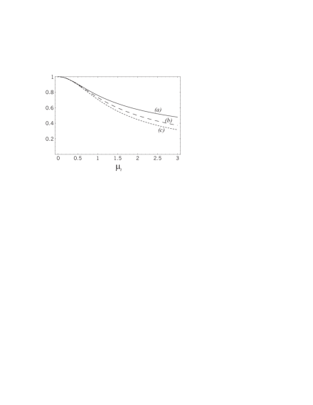
FIG. 3.: (a) Square root of the CPP state purity parameter $\sqrt{P_{\rm temp}(\mu_{t})}$ which sets the maximum achievable level of mode matching for a given optical arrangement; (b) temporal mode overlap $M(\mu_{t},\mu_{A}^{\rm max})$ between the DFG and CPP modes for the optimally chosen alignment beam; (c) temporal mode overlap $M(\mu_{t},0)$ for a plane wave alignment beam.

B Time-space representation

To gain a further insight into the phenomena considered in this paper we calculate the CPP mode purity parameter in the space-time representation rather than the frequency-momentum representation we used so far. In this subsection we work with correlation functions defined as $\tilde{\Gamma}({\mathbf{r}},t,{\mathbf{r}}^{\prime},t^{\prime})=\left<\tilde{E}^{(-)}({\mathbf{r}},t)\,\tilde{E}^{(+)}({\mathbf{r}}^{\prime},t^{\prime})\right>$, with the mode matching and purity parameters redefined analogously.

We employ the same assumptions as in the previous subsection but do the calculation for the spatial domain. To facilitate visualizing the physics involved, we utilize Klyshko’s advanced wave model and perform the entire calculation classically.

The transverse correlation function of the DFG mode is obtained from Eq. (23) and is as follows:

$$\tilde{\Gamma}_{s}({\mathbf{r}},{\mathbf{r}}^{\prime})=|\beta|^{2}\tilde{E}_{p}^{(-)}({\mathbf{r}})\tilde{E}_{p}^{(+)}({\mathbf{r}}^{\prime})\tilde{\Gamma}_{t}^{*}({\mathbf{r}},{\mathbf{r}}^{\prime}),$$ (40)

where ${\mathbf{r}}$ denotes the transverse radius vectors in the crystal plane and $\tilde{\Gamma}_{t}({\mathbf{r}},{\mathbf{r}}^{\prime})$ is the correlation function of the advanced wave in the plane of the crystal. In writing this equation we made use of the fact that the pump pulse is a coherent wave.

The photon counter behind the spectral filter pinhole is replaced, according to the Klyshko model, by a source generating spatially incoherent light backwards in space and time. The light emitted by the source passes through the pinhole and is collimated by the focusing lens (Fig. 2(b)). The correlation function of the advanced wave in the plane of the nonlinear crystal is then equal to that in the plane of the focusing lens. The latter is determined in the far-field approximation using the Van Cittert-Zernike theorem [20]:

$$\tilde{\Gamma}_{t}({\mathbf{r}},{\mathbf{r}}^{\prime})=\int T({\mathbf{R}})e^{-i(k_{t}/F){\mathbf{R}}\cdot({\mathbf{r}}-{\mathbf{r}}^{\prime})}d^{3}R,$$ (41)

where $k_{t}=2\pi/\lambda_{t}$ is the trigger wavenumber, $F$ is the focal length of the lens and $T({\mathbf{R}})$ is the pinhole transmission.

1 Gaussian filter

For a Gaussian filter (33), replacing ${\mathbf{k}}_{\bot}=k_{t}{\mathbf{R}}/F$ and performing a Fourier transform according to Eq. (41) we obtain the correlation function of the advanced wave:

$$\tilde{\Gamma}_{t}({\mathbf{r}},{\mathbf{r}}^{\prime})=\tilde{\Gamma}_{t}^{0}\exp\left(-(\kappa_{t}|{\mathbf{r}}-{\mathbf{r}}^{\prime}|/2)^{2}\right).$$ (42)

Substituting it into Eq.(40) and writing for the pump field (32) $\tilde{E}_{p}^{(+)}({\mathbf{r}})\propto\exp(-(\kappa_{p}|{\mathbf{r}}|/2)^{2})$, we determine the spatial correlation function of the signal mode and its purity parameter:

$$P_{\rm sp}=\frac{\int d^{3}r\,d^{3}r^{\prime}\,\tilde{\Gamma}_{s}({\mathbf{r}},{\mathbf{r}}^{\prime})\tilde{\Gamma}_{s}^{*}({\mathbf{r}},{\mathbf{r}}^{\prime})}{(\int d^{3}r\,\tilde{\Gamma}_{s}({\mathbf{r}},{\mathbf{r}}))^{2}}=\frac{1}{1+2\kappa_{t}^{2}/\kappa_{p}^{2}}.$$ (43)

This expression is clearly analogous to Eq. (36). The absence of a square root is explained by the two-dimensional character of spatial mode matching.

The light emitted by Klyshko’s virtual source is completely incoherent. However, as the advanced wave passes through a narrow aperture, it gains some degree of transverse coherence according to the Van Cittert-Zernike theorem. Because the nonlinear interaction is restricted to the area where the pump field is present, the resulting signal (DFG) field is also partially coherent provided the pump beam diameter is smaller than the transverse coherence length of the advanced wave. This explains why the advanced wave, in spite of its own incoherence, may generate a highly coherent CPP signal.

2 Cylindrical filter

To make the above calculation more useful for practical applications, consider a spatial filter not of Gaussian shape, but of top-hat shape, i.e. the pinhole transmits all the light within its radius $\rho$. In this case, the correlation function of the advanced wave, calculated using Eq. (41), is given by

$$\Gamma_{t}({\mathbf{r}},{\mathbf{r}}^{\prime})=\frac{2J_{1}(k_{t}\rho|{\mathbf{r}}-{\mathbf{r}}^{\prime}|/F)}{(k_{t}\rho|{\mathbf{r}}-{\mathbf{r}}^{\prime}|/F)},$$ (44)

where $J_{1}(x)$ is the first order Bessel function. Approximating $2J_{1}(x)/x\approx 1-x^{2}/8$ for small $x$ and comparing the correlation functions (42) and (44) we find that the two functions behave similarly on small spatial scales if $\kappa_{t}=k_{t}\rho/(F\sqrt{2})$. Substituting the latter identity into Eq. (43) and expressing $\kappa_{p}$ through the FWHM diameter $d_{p}$ of the pump beam ($\kappa_{p}=2\sqrt{2\ln 2}/d_{p}$) we find in the limit of tight filtering

$$P_{\rm sp}\approx 1-\left(\frac{\pi\rho d_{p}}{\sqrt{2\ln 2}\lambda_{t}F}\right)^{2},$$ (45)

where $\lambda_{t}$ is trigger wavelength. Equations (37) and (45) provide the means for evaluating the CPP mode purity factor from a set of parameters that are readily measurable in an experiment. The mode matching efficiency is then evaluated using inequality (22).

VI Experimental considerations

As we have shown in the previous section, tight filtering in the trigger channel, both spatial and temporal, is the key to obtaining a CPP ensemble which approaches a pure state and can be coupled into a classical optical mode. In experimental practice, reducing the width of spatial and spectral filters lowers the trigger count rate and increases the relative fraction of dark counts. As seen from Eq. (37), a reasonable compromise (dependent on a particular application) is a spectral filter FWHM on the order of the inverse duration of the pump pulse. A favorable size for the pinhole in the spatial filter is obtained from Eq. (45) and should be such that the imaginary coherent wave propagating backwards through the pinhole would create a diffraction spot in the optical plane of the crystal which is several times larger than the diameter of the pump beam.

An important experimental limitation is imposed by the existing technology of making optical coatings. Interference bandpass filters narrower than 1 $\rm\AA$ are not available or very expensive. Ultrashort (less than a few picoseconds) laser pulses must therefore be used to pump the downconverter so that the trigger filter bandwidth can be made sufficiently narrow in comparison with the pump linewidth.

The freedom of choice of the optimally matching classical pulse is also limited. While its spatial parameters can be varied in a wide range, its temporal width is set by the master laser and cannot be changed easily. Using laser pulses of non-optimal width results in a reduction of the temporal mode matching efficiency. If the width of the matching Gaussian pulse differs from that of the CPP mode by a factor of $\alpha$, the mode matching is reduced by a factor of

$$f(\alpha)=\frac{2\alpha}{\alpha^{2}+1}.$$ (46)

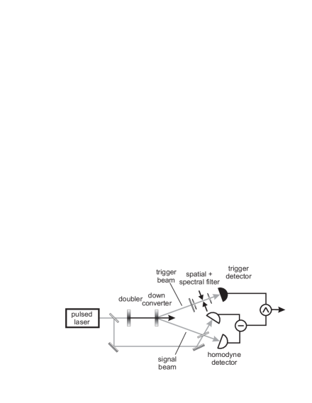
FIG. 4.: Scheme of the experiment on quantum tomography of single-photon states

As a practical example of solving the mode matching problem we consider the experiment of Lvovsky et al. [13] on homodyne tomography of the single-photon Fock state (Fig. 4). In this experiment, $\lambda=790$ nm, $\sqrt{2}\tau_{p}=$1.6 ps master laser pulses were frequency doubled and then down-converted in a type-I frequency degenerate configuration. Such a scheme permitted to use a fraction of the original laser radiation as the local oscillator for the balanced homodyne detector. The photons emitted into the trigger channel were filtered by a combination of a $0.4$-nm ($w_{t}=1.2\times 10^{12}\ \rm{s}^{-1}$) FWHM interference filter and a spatial filter consisting of a $F=80$ mm focal length lens and a $2\rho=50$ $\mu$m pinhole. The FWHM diameter of the pump beam was $d_{p}=0.34$ mm. The laser frequency was centered at the transmission peak of the spectral filter which insured the coincidence of the center frequencies of the CPP and the local oscillator (LO).

In order to perform an efficient homodyne measurement it was necessary to achieve good mode overlap between the local oscillator and the CPP. Since at the time of the measurement no alignment beam could have been present in the trigger channel, the procedure of preparing the matching classical mode described in Section IV was applied in two steps. In the first step, a fraction of the master laser field was inserted into the trigger channel and synchronized with the pump pulses. This field generated DFG emission through its nonlinear interaction with the pump and thus fulfilled the function of the alignment beam. The LO beam was overlapped with the DFG beam on a 50-% beamsplitter and interference between the two classical fields was observed in one of the beamsplitter output ports. The visibility of the interference pattern was maximized by varying the spatial parameters of the LO beam with a 3-lens telescope and steering mirrors. In the second step, the alignment beam was blocked and a tomography measurement was performed using the same beamsplitter for balanced homodyning.

The task of evaluating the mode matching between the LO and CPP modes thus splits into two parts. First, the purity parameter $P$ of the CPP mode needs to be evaluated $theoretically$ to establish the upper limit for the mode matching between the CPP and DFG waves. Second, the level of mode matching $M_{\rm cl}$ between the classical DFG and LO waves has to be determined $experimentally$ from the visibility of the interference pattern. The overlap between the CPP and LO modes can then be evaluated as a product $M=M_{\rm cl}\sqrt{P}$.

Although the down-conversion occurred in a non-collinear configuration, the angle between the down-conversion channels and the pump beam was relatively small ($6.8^{\circ}$) so the approximations outlined in the beginning of Section V were applicable to the system. The signal beam walk-off was eliminated by using the “hot spot” configuration of the down-converter [21] and the group velocity dispersion effects were negligible [22]. Applying Eqs. (37) and (45) to the actual experimental parameters we find the values of $P_{\rm temp}=0.85$ and $P_{\rm sp}=0.87$ for the temporal and spatial purity parameters of the CPP mode, respectively. This corresponds to a maximum achievable mode matching efficiency of $\sqrt{P}=\sqrt{P_{\rm temp}P_{\rm sp}}=0.86$.

The maximum visibility of the interference fringes observed between the DFG and LO waves was equal to 0.83 which corresponds to a mode matching factor $M_{\rm exp}=0.69$. In order to obtain $M_{\rm cl}$, this value needs to be corrected to accommodate for the temporal properties of the alignment pulse. While its $spatial$ characteristics were optimized according to the requirements established in Section V (the alignment beam was made broad and collimated so it passed well through the spatial filter), its $temporal$ properties were beyond our control. The alignment field was not narrowband (as required), which resulted in a different linewidth of the DFG field as compared to the CPP mode. The nonlinear interaction between the second harmonic (pump) and the fundamental (alignment) waves produces a DFG wave whose linewidth is broader by a factor $\sqrt{3}$ than the fundamental. On the other hand, the spectral linewidth of the CPP mode in the limit of narrow filtering would mimic that of the pump, which is $\sqrt{2}$ times the fundamental [12]. If a narrowband alignment beam were available, the mode overlap between the LO and DFG waves would have been by a factor of $f(\sqrt{2})/f(\sqrt{3})=1.09$ higher than the one actually observed. We find $M_{\rm cl}=M_{\rm exp}f(\sqrt{2})/f(\sqrt{3})=0.75$.

We calculate the overall factor of spatiotemporal mode matching between the LO and CPP waves as $M=\sqrt{P}\times M_{\rm cl}=0.65$. This number is in agreement with the value of $0.69\times 0.95$ quoted in Ref. [13].

VII Conclusion

We have investigated the spatiotemporal optical mode of the single-photon Fock state prepared by conditional measurements on a biphoton born in the process of parametric down-conversion and the possibilities of matching it with a classical wave. Our theory, developed using the density-matrix formalism, shows that in order to obtain a pure single-photon state in the signal channel it is essential to provide narrow spatiotemporal filtering in the trigger channel. Only in this case can efficient mode matching be achieved. The theoretical limit of mode matching can be expressed in terms of the CPP mode purity factor which is readily determined as a function of the experimental parameters.

We have shown that the optical mode of the CPP is identical to that of a classical wave generated due to a nonlinear interaction of the pump wave and Klyshko’s advanced wave. Based on this knowledge we proposed and implemented an experimental method of modeling the CPP mode by using a narrowband alignment beam in place of the advanced wave. The difference frequency field generated in such an arrangement matches the CPP mode with an efficiency that approaches the theoretical limit.

Finally, we have discussed how the mode matching efficiency can be evaluated and optimized in a practical experimental arrangement.

This project is sponsored by the Deutsche Forschungsgemeinschaft. A. L. is supported by the Alexander von Humboldt foundation. We thank Prof. J. Mlynek and Dr. H. Hansen for helpful discussions.

REFERENCES

- [1] For a review, see W. Tittel, G. Ribordy and N. Gisin, Physics World, March 1998, page 41
- [2] E. Knill, R. Laflamme, and G. Milburn, Nature 409, 46, 2001
- [3] see, for example, S. Haroche et al., Nature 400, 239 (1999); B. T. H. Varcoe, S. Brattke et al., Nature 403, 743 (2000)]; Y. Yamamoto et al., Nature 397, 500 (1999)]; M. Hennrich et al., Phys. Rev. Lett. 85, 4872 (2000) and articles on single photon generation in this issue of Eur. Phys. J.
- [4] C. K. Hong and L. Mandel, Phys. Rev. Lett. 56, 58 (1986)
- [5] P. Grangier, G. Roger and A. Aspect, Europhys. Lett. 1, 173 (1986)
- [6] see, for example, D. Stoler, B. Yurke, Phys. Rev. A 34, 3143 (1986); J.G. Rarity, P.R. Tapster, Phys. Rev. A 59, 35 (1999); P. Kwiat et al, Phys. Rev. Lett. 74, 4763 (1995)
- [7] A. Joobeur, B.E.A. Saleh, M.C. Teich, Phys. Rev. A 50, 3349 (1994);
- [8] T. B. Pittman, D. V. Strekalov, D. N. Klyshko, M. H. Rubin, A. V. Sergienko, and Y. H. Shih, Phys. Rev. A 53, 2804-2815 (1996);
- [9] M. Atature et al., Phys. Rev. Lett. 1323 (1999)
- [10] D. Branning et al., Phys. Rev. Lett. 83,955 (1999)
- [11] Z. Y. Ou, Qu. Semiclass. Opt. 9, 599 (1997)
- [12] F. Grosshans and P. Grangier, Eur. Phys. J. D 14, 119 (2001)
- [13] A. I. Lvovsky et al, Phys Rev. Lett. 87, 050402 (2001)
- [14] C. Kurtsiefer, M. Oberparleiter, and H. Weinfurter, Phys. Rev. A 64, 023802 (2001)
- [15] Z. Y. Ou, L. J. Wang, and L. Mandel, Phys. Rev. A 40, 1428 (1989)
- [16] W. E. Lamb, Appl. Phys. 60, 77 (1995)
- [17] D. N. Klyshko, Phys. Lett. A 132, 299 (1988); D. N. Klyshko, Phys. Lett. A 128, 133 (1988); D. N. Klyshko, Sov. Phys. Usp., 31 74, (1988).
- [18] C. H. Bennett et al., quant-ph/0006044
- [19] C. K. Hong, Z. Y. Ou, and L. Mandel, Phys. Rev. Lett. 59, 2044 (1987)
- [20] M. Born and E. Wolf, Principles of optics, Pergamon, 1964
- [21] K. Koch et al., IEEE J. Quant. El. 31, 769 (1995)
- [22] H. Hansen, PhD thesis (Universität Konstanz, 2000)