Universal dynamical control of quantum mechanical decay: Modulation of the coupling to the continuum

Abstract

We derive and investigate an expression for the dynamically modified decay of states coupled to an arbitrary continuum. This expression is universally valid for weak temporal perturbations. The resulting insights can serve as useful recipes for optimized control of decay and decoherence.

The quantum Zeno effect (QZE), namely, the inhibition of the decay of an unstable state by its (sufficiently frequent) projective measurements, has long been considered a basic universal feature of quantum systems [1]. Our general analysis [2] has revealed the inherent impossibility of the QZE for a broad class of processes, including spontaneous emission in open space, as opposed to the ubiquitous occurrence of the anti-Zeno effect (AZE), i.e., decay acceleration by frequent projective measurements [3]. Although realistic schemes may well approximate such measurements [2, 4, 5], there is strong incentive for raising the question: Are projective measurements the most effective way of modifying the decay of an unstable state? This question is prompted by two important results: (a) A landmark experiment has demonstrated, for the first time, both the QZE and AZE by repeated on-off switching of the coupling between a nearly bound state and the continuum, using cold atoms that are initially trapped in an optical-lattice potential [6]. (b) It has been predicted that periodic coherent pulses, acting between the decaying level and an auxiliary one, can either inhibit or accelerate the decay into certain model reservoirs [7]. In both [6] and [7], the repeated interruption of the “natural” evolution is imperative for decay modification.

In this paper we purport to substantially expand the arsenal of decay control, whether measurement-like (i.e., accompanied by dephasing) or fully coherent. We derive a universal form of the decay rate of unstable states into any reservoir (continuum), modified by weak perturbations with arbitrary time dependence. The results of Refs. [2, 3, 6, 7] are recovered as limiting cases of this universal form. Our analysis can serve as a general recipe for optimized decay and decoherence suppression for quantum logic operations [8] or decay enhancement for the control of chaos or chemical reactions [9].

Consider the decay of a state $|e\rangle$ via its coupling to a system, described by the orthonormal basis $\{|j\rangle\}$, which forms either a discrete or a continuous spectrum (or a mixture thereof). In its most general form, the total Hamiltonian is $\hat{H}_{0}+\hat{V}(t)+H_{1}(t)$, where

$$\hat{H}_{0}=\hbar\omega_{a}|e\rangle\langle e|+\hbar\sum_{j}\omega_{j}|j\rangle\langle j|,$$ (1)

with $\hbar\omega_{a}$ and $\hbar\omega_{j}$ being the energies of $|e\rangle$ and $|j\rangle$, respectively;

$$\hat{V}(t)=\sum_{j}V_{ej}(t)|e\rangle\langle j|+\text{h.c.},$$ (2)

denoting the off-diagonal coupling of $|e\rangle$ with the other states, which is dynamically modulated, so as to modify the static limit of $\hat{V}$ effecting the natural decay process; and

$$H_{1}(t)=\hbar\delta_{a}(t)|e\rangle\langle e|+\hbar\sum_{j}\delta_{j}(t)|j\rangle\langle j|,$$ (3)

standing for the adiabatic (diagonal) time-dependent perturbations of the energies of the initial ($|e\rangle$) and final ($|j\rangle$) states, e.g., AC Stark shifts.

We write the wave function of the system, with $|e\rangle$ populated at $t=0$, as

$$|\Psi(t)\rangle= \alpha(t)e^{-i\omega_{a}t-i\int_{0}^{t}\delta_{a}(t^{\prime})dt^{\prime}}|e\rangle$$ (5)

$$+\sum_{j}\beta_{j}(t)e^{-i\omega_{j}t-i\int_{0}^{t}\delta_{j}(t^{\prime})dt^{\prime}}|j\rangle,$$

the initial condition being $|\Psi(0)\rangle=|e\rangle$. Henceforth we treat the generic case wherein the level shifts and the temporal modulation of $\hat{V}(t)$ are independent of $j$, i.e., $\delta_{j}(t)\equiv\delta_{f}(t)$ and $V_{je}(t)\equiv\tilde{\epsilon}(t)\mu_{je}$, $\tilde{\epsilon}(t)$ being the modulation function (Fig. 1 – inset). Such factorized form of the modulation is commonly valid for weak or moderate time-dependent fields, which do not appreciably change the states of the continuum. One then obtains from the Schrödinger equation that the amplitude $\alpha(t)$ obeys the exact integro-differential equation [10]

$$\dot{\alpha}=-\int_{0}^{t}dt^{\prime}\epsilon^{*}(t)\epsilon(t^{\prime})\Phi(t-t^{\prime})e^{i\omega_{a}(t-t^{\prime})}\alpha(t^{\prime}).$$ (6)

Here $\Phi(t)=\hbar^{-2}\sum_{j}|\mu_{ej}|^{2}e^{-i\omega_{j}(t)}$ is the reservoir response (memory) function and the function $\epsilon(t)=\tilde{\epsilon}(t)\exp[-i\int_{0}^{t}\delta_{af}(t^{\prime})dt^{\prime}]$, with $\delta_{af}(t)=\delta_{a}(t)-\delta_{f}(t)$, accounts for the modulation of either diagonal or off-diagonal elements of the unperturbed Hamiltonian.

The assumption that the coupling (2) is a weak perturbation of (1) implies that $\alpha(t)$ varies sufficiently slowly with respect to the kernel of Eq. (6), since we then anticipate [cf. the validity condition (13)] decay rates much smaller than the rate of change of the reservoir response $\Phi(t)$. One can thus make the approximation $\alpha(t^{\prime})\approx\alpha(t)$ on the right-hand side (rhs) of Eq. (6). Then one can solve Eq. (6) and represent the amplitude modulus of level $|e\rangle$ in the form

$$|\alpha(t)|=\exp[-R(t)Q(t)/2],$$ (7)

where we have introduced the fluence $Q(t)=\int_{0}^{t}d\tau|\epsilon(\tau)|^{2}$, and obtained the decay rate in the universal form

$$R(t)=2\pi\int_{-\infty}^{\infty}d\omega G(\omega+\omega_{a})F_{t}(\omega).$$ (8)

Here $G(\omega)=\pi^{-1}\text{Re}\int_{0}^{\infty}dte^{i\omega t}\Phi(t)=\hbar^{-2}\sum_{j}|\mu_{ej}|^{2}\delta(\omega-\omega_{j})$ is the coupling spectrum, i.e., the density of states weighted by the strength of the coupling to the continuum or reservoir; $F_{t}(\omega)=|\epsilon_{t}(\omega)|^{2}/Q(t)$, with $\epsilon_{t}(\omega)=(2\pi)^{-1/2}\int_{0}^{t}\epsilon(t^{\prime})e^{i\omega t^{\prime}}dt^{\prime}$, is the (normalized to unity) spectrum of the modulation function $\epsilon(t)$ in the “window” $(0,t)$. The result (7), (8) is valid to all orders of $t$, i.e., it keeps intact the interferences between the modulated decay channels and their non-Markovian effects. We stress that Eqs. (7), (8) apply to the decay of superposed states $\sum_{m}\alpha_{m}|e_{m}\rangle$ (e.g., in quantum information schemes), provided all of them decay and are modulated identically.

We now consider some important consequences of the universal form (7), (8). The modulation spectrum $F_{t}(\omega)$ is roughly characterized by its width $\nu_{t}$ and the frequency shift $\Delta_{t}=\int d\omega\omega F_{t}(\omega)$. A modulation may strongly modify the decay rate (analogously to the QZE or AZE) whenever $\nu_{t}+|\Delta_{t}|\gtrsim\xi(\omega_{a})$, where $\xi(\omega_{a})$ is the characteristic spectral interval over which the weighted density of states $G(\omega)$ changes near $\omega_{a}$. In particular, if $\omega_{a}$ is near the edge of the continuum (as for radiative decay in photonic crystals or vibrational decay in ion traps, molecules and solids), then $\xi(\omega_{a})$ is the distance between $\omega_{a}$ and the edge [2] (Fig. 1a). Only in the opposite limit, $\nu_{t}+|\Delta_{t}|\ll\xi(\omega_{a})$, can one approximately set $F_{t}(\omega)\approx\delta(\omega)$ in Eq. (8), yielding $P(t)\approx\exp[-R_{\rm GR}Q(t)]$, where $R_{\rm GR}=2\pi G(\omega_{a})$ is the extension of the Golden-Rule (GR) rate to the case of a time-dependent coupling.

The modulation function $\epsilon(t)$ can be either random or regular (coherent) in time, as detailed below. Consider first the most general coherent amplitude and phase modulation (APM) of the quasiperiodic form, $\epsilon(t)=\sum_{k}\epsilon_{k}e^{-i\omega_{k}t}$. Here $\omega_{k}$ ($k=0,\pm 1,\dots$) are arbitrary discrete frequencies with the minimum spectral distance $\Omega$. For a given function $\epsilon(t)$ one can obtain $-i\omega_{k}$ and $\epsilon_{k}$ as the poles and residues, respectively, of the Laplace transform $\hat{\epsilon}(s)$. If $\epsilon(t)$ is periodic with the period $\Omega$, then $\omega_{k}=k\Omega$, and $\epsilon_{k}$ become the Fourier components of $\epsilon(t)$. For a general quasiperiodic $\epsilon(t)$, one obtains

$$Q(t)=\epsilon_{c}^{2}t+\epsilon_{c}^{2}\sum_{k\neq l}\lambda_{k}\lambda_{l}^{*}\frac{e^{i(\omega_{l}-\omega_{k})t}-1}{i(\omega_{l}-\omega_{k})},$$ (9)

where $\epsilon_{c}^{2}=\sum_{k}|\epsilon_{k}|^{2}$ equals the average of $|\epsilon(t)|^{2}$ over a period of the order of $1/\Omega$, $\lambda_{k}=\epsilon_{k}/\epsilon_{c}$ and

$$|\epsilon_{t}(\omega)|^{2}=\epsilon_{c}^{2}t\sum_{k}|\lambda_{k}|^{2}S(\eta_{k}t/2)$$ (10)

$$+\epsilon_{c}^{2}\sum_{k\neq l}\lambda_{k}\lambda_{l}^{*}\frac{1+e^{i(\omega_{l}-\omega_{k})t}-e^{i\eta_{k}t}-e^{-i\eta_{l}t}}{2\pi\eta_{k}\eta_{l}}.$$ (11)

Here $\eta_{k}=\omega-\omega_{k}$, whereas $S(\eta_{k}t/2)=2\sin^{2}(\eta_{k}t/2)/\pi t\eta_{k}^{2}$ is a sinc-function of $\eta_{k}$ normalized to 1.

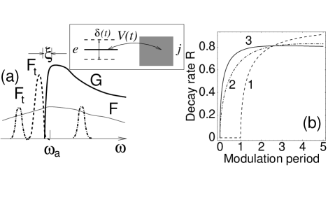
FIG. 1.: Decay modification by modulation [Eqs. (7), (8)]. Inset: Schematic view of the temporal modulation of the shift of level $e$ and its coupling to a continuum. (a) $\omega_{a}$ is near a band edge of $G(\omega)=C\omega^{1/2}(\omega+\Gamma)^{-1}\theta(\omega)$, where $\theta(\omega)$ is the unit step function; then a small phase shift (dashed peak) is more effective in reducing the decay rate $R$ than large phase shifts $\phi\simeq\pi$ (dash-dotted peaks) or frequent measurements/random $\epsilon(t)$ (thin curve). (b) Decay rate $R$ (in units of $R_{\rm GR}$) in case (a) with $\omega_{a}=0.1\Gamma$: reduction by PM [Eq. (12)] (curve 1 – $\phi=0.1$, curve 2 – $\phi=\pi$) and frequent impulsive measurements [2] (curve 3 – QZE) as a function of perturbation period $\tau$ (in units of $\Gamma^{-1}$). Curve 1 gives the strongest reduction of $R$ at a given $\tau$.

For $t\gg\Omega^{-1}$ the first term on the rhs of (11) is a sum of peaks, whose spacings are much greater than their width $2/t$. The fast oscillating second term is also peaked at $\omega=\omega_{k}$, but we then find that the ratio of the first to the second terms, and that of their counterparts in (9), is $\sim(\Omega t)^{-1}\ll 1$. In the long-time limit, we then neglect these fast oscillating terms and obtain from Eqs. (7)-(11) that $P(t)=\exp[-R(t)\epsilon_{c}^{2}t]$, where $R(t)$ in Eq. (8) now involves $F_{t}(\omega)\approx\sum_{k}|\lambda_{k}|^{2}S(\eta_{k}t/2)$. For even longer times, exceeding the effective correlation (memory) time of the reservoir, $t_{c}\equiv\max_{k}\{1/\xi(\omega_{a}+\omega_{k})\}$, the functions $S(\eta_{k}t/2)$ become narrower than the respective characteristic widths of $G(\omega)$ around $\omega_{a}+\omega_{k}$, and one can set $S(\eta_{k}t/2)\approx\delta(\eta_{k})$. Then Eq. (8) is reduced to

$$R=2\pi\sum_{k}|\lambda_{k}|^{2}G(\omega_{a}+\omega_{k}),$$ (12)

which holds if

$$Rt_{c}\ll 1.$$ (13)

This condition is well satisfied in the regime of interest, i.e., weak coupling to essentially any reservoir, unless (for some $k$) $\omega_{a}+\omega_{k}$ is extremely close to a sharp feature in $G(\omega)$, e.g., a band edge [11]. Hence, the long-time limit of the general decay rate (8) under the APM is a sum of the GR rates, corresponding to the resonant frequencies shifted by $\omega_{k}$, with the weights $|\lambda_{k}|^{2}$. Formula (12) provides a simple general recipe for manipulating the decay rate by APM. Its powerful generality allows for the optimized control of decay, not just for a single level, but also for band characterized by a spectral distribution $P(\omega_{a})$ (e.g., inhomogeneous or vibrational spectrum). We can then choose $\lambda_{k}$ and $\omega_{k}$ in Eq. (12) so as to minimize the decay of (7) convoluted with $P(\omega_{a})$. The following limits of (12) will be now analyzed.

(i) Monochromatic perturbation: Let $\epsilon(t)=\epsilon_{0}e^{-i\delta_{af}t}$. Then $R=2\pi G(\omega_{a}+\Delta)$, where $\Delta=\delta_{af}=\text{const}$ is an AC Stark shift. In principle, such a shift may drastically enhance or suppress $R$ relative to $R_{\rm GR}$. It provides the maximal variation of $R$ achievable with an external perturbation, since it does not involve any averaging (smoothing) of $G(\omega)$ incurred by the width of $F_{t}(\omega)$: the modified $R$ can even vanish, if the shifted frequency $\omega_{a}+\Delta$ is beyond the cutoff frequency of the coupling, where $G(\omega)=0$ (Fig. 1a,b). Conversely, the increase of $R$ due to a shift can be much greater than that achievable with the AZE [2]. In practice, however, AC Stark shifts are usually small for (CW) monochromatic perturbations, whence pulsed perturbations should often be used, resulting in multiple $\omega_{k}$ shifts according to (12).

(ii) Impulsive phase modulation (PM): Let the phase of the coupling amplitude jump by an amount $\phi$ at times $\tau,2\tau,\dots$. Such modulation can be achieved by a train of identical, equidistant, narrow pulses of nonresonant radiation, which produce pulsed AC Stark shifts $\delta_{af}(t)$ in (3). Now $\epsilon(t)=e^{i[t/\tau]\phi}$, where $[\dots]$ is the integer part. One then obtains that $\epsilon_{c}=1$ and $Q(t)=t$. The decay is given by Eqs. (7) and (8), where $F_{t}(\omega)$ can be obtained in a closed form. For sufficiently long times one can use Eq. (12). The poles and residues of $\hat{\epsilon}(s)=(1-e^{-s\tau})/[s(1-e^{i\phi-s\tau})]$ yield $\omega_{k}=2k\pi/\tau-\phi/\tau$ and $|\lambda_{k}|^{2}=4\sin^{2}(\phi/2)/(2k\pi-\phi)^{2}$. For small phase shifts, $\phi\ll 1$, the $k=0$ peak dominates, $|\lambda_{0}|^{2}\approx 1-\phi^{2}/12$, whereas $|\lambda_{k}|^{2}\approx\phi^{2}/4\pi^{2}k^{2}$ for $k\neq 0$. In this case one can retain only the $k=0$ term in Eq. (12) [unless $G(\omega)$ is changing very fast]. Then the modulation acts as a constant shift $\Delta=-\phi/\tau$. With the increase of $|\phi|$, the difference between the $k=0$ and $k=1$ peak heights diminishes, vanishing for $\phi=\pm\pi$. Then $|\lambda_{0}|^{2}=|\lambda_{1}|^{2}=4/\pi^{2}$, i.e., $F_{t}(\omega)$ for $\phi=\pm\pi$ contains two identical peaks symmetrically shifted in opposite directions (Fig. 1a) [the other peaks $|\lambda_{k}|^{2}$ decrease with $k$ as $(2k-1)^{-2}$, totaling 0.19].

The above features allow one to adjust the modulation parameters for a given scenario to obtain an optimal decrease or increase of $R$. The PM scheme with a small $\phi$ is preferable near the continuum edge (Fig. 1a,b), since it yields a spectral shift in the required direction (positive or negative). The adverse effect of $k\neq 0$ peaks in $F_{t}(\omega)$ then scales as $\phi^{2}$ and hence can be significantly reduced by decreasing $|\phi|$. On the other hand, if $\omega_{a}$ is near a symmetric peak of $G(\omega)$, $R$ is reduced more effectively for $\phi\simeq\pi$, as in Ref. [7], since the main peaks of $F_{t}(\omega)$ at $\omega_{0}$ and $\omega_{1}$ then shift stronger with $\tau^{-1}$ than the peak at $\omega_{0}=-\phi/\tau$ for $\phi\ll 1$.

(iii) Amplitude modulation (AM) of the coupling arises, e.g., for radiative-decay modulation due to atomic motion through a high-$Q$ cavity or a photonic crystal [12] or for atomic tunneling in optical lattices with time-varying lattice acceleration [6, 13]. Let the coupling be turned on and off periodically, for the time $\tau_{1}$ and $\tau_{0}-\tau_{1}$, respectively, i.e., $\epsilon=1$ for $n\tau_{0}<t<n\tau_{0}+\tau_{1}$ and $\epsilon=0$ for $n\tau_{0}+\tau_{1}<t<(n+1)\tau_{0}$ ($n=0,1,\dots$). Now $Q(t)$ in (7) is the total time during which the coupling is switched on. This case is also covered by Eq. (12), where the parameters are now found to be $\epsilon_{c}^{2}=\tau_{1}/\tau_{0}$, $\omega_{k}=2k\pi/\tau_{0}$, $|\lambda_{0}|^{2}=\tau_{1}/\tau_{0}$, $|\lambda_{k}|^{2}=(\tau_{1}/\tau_{0})\text{sinc}^{2}(k\pi\tau_{1}/\tau_{0})$ ($k\neq 0$).

It is instructive to consider the limit wherein $\tau_{1}\ll\tau_{0}$ and $\tau_{0}$ is much greater than the correlation time of the continuum, i.e., $G(\omega)$ does not change significantly over the spectral intervals $(2\pi k/\tau_{0},2\pi(k+1)/\tau_{0})$. In this case one can approximate the sum (12) by the integral (8) with $F_{t}(\omega)\approx(\tau_{1}/2\pi)\text{sinc}^{2}(\omega\tau_{1}/2)$, characterized by the spectral broadening $\sim 1/\tau_{1}$ (Fig. 2 – inset). Then Eq. (8) for $R$ reduces to that obtained when ideal projective measurements are performed at intervals $\tau_{1}$ [2].

Thus the AM scheme can imitate measurement-induced (dephasing) effects on quantum dynamics, if the interruption intervals $\tau_{0}$ exceed the correlation time of the continuum. This indeed has been observed [6] for atom tunneling in optical lattices whose tilt (acceleration) was periodically modulated as above. For its analysis we have used the approximate expression for $\Phi(t)$ obtained in [13], which yields the reservoir spectrum $G(\omega+\omega_{a})$ (Fig. 2 – inset), with one maximum at $\omega\sim\omega_{g}$, $\hbar\omega_{g}$ being the lattice band gap. The decay probability $P(t)$, calculated in Fig. 2 (curves 1-4) for parameters similar to [6], completely coincides with that obtained for ideal impulsive measurements at intervals $\tau_{1}$ [2] and demonstrates either the QZE (curve 2) or the AZE (curve 3) behavior.

The universal Eq. (8), which is a result of unitary analysis, is valid also when $\epsilon(t)$ is a stationary random process. If such a process is characterized by the correlation time $\nu^{-1}$, one can use a master equation to show that, for $t\gg\nu^{-1}$, we have $P(t)\approx e^{-Rt}$, where the decay rate (provided that $R\ll\nu$) still has the general form (8), but with

$$F_{t}(\omega)\rightarrow F(\omega)=\pi^{-1}\epsilon_{c}^{-2}{\hbox{Re}}\int_{0}^{\infty}\overline{\epsilon^{*}(t)\epsilon(0)}e^{i\omega t}dt,$$ (14)

$F(\omega)$ being the normalized spectrum of the random process and $\epsilon_{c}^{2}=\overline{|\epsilon(t)|^{2}}$, where the overbar denotes ensemble averaging. Expression (8) with the substitution (14) is completely analogous to the universal formula describing measurement effects on quantum evolution in [2]. This analogy between unitary and measurement effects stems from the ability to emulate projective measurements by the dephasing of the level evolution caused by classical random fields [2, 5].

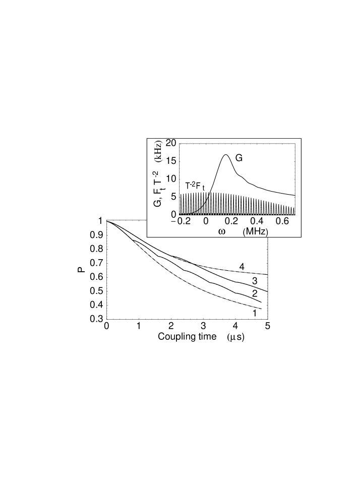
FIG. 2.: Tunneling of sodium atoms in optical lattices perturbed by AM scheme: the decay probability $P(t)$ as a function of the total coupling time. Curves 1, 4 – decay without modulation. Curve 2 – QZE (decay slowdown compared to curve 1) for $\tau_{1}=0.8\ \mu$s, $\tau_{0}=50.8\ \mu$s. Curve 3 – AZE (decay speedup compared to curve 4) for $\tau_{1}=2\ \mu$s, $\tau_{0}=52\ \mu$s. Inset: The coupling spectrum $G(\omega+\omega_{a})$ and the scaled modulation function $T^{-2}F_{4\tau_{0}}(\omega)$ for the conditions of curve 2. Here $T=\omega_{g}d/(\pi a)$, where $a=15$ km/s² is the lattice acceleration and $d=295$ nm is the lattice period. $\omega_{g}=91$ kHz, $\omega_{g}T=2.05$ (for curves 1, 2, 5); $\omega_{g}=116$ kHz, $\omega_{g}T=3.32$ (for curves 3, 4).

There may, however, be a notable difference between projections and random-field dephasing. Projective measurements at an effective rate $\nu$, whether impulsive or continuous, usually result in a broadened (to a width $\nu$) modulation function $F(\omega)$, without a shift of its center of gravity, $\Delta=\int d\omega\omega F(\omega)\approx 0$ [2, 4]. This feature was shown [2] to be responsible for either the standard QZE scaling, $R\sim 1/\nu$, or the AZE scaling. In contrast, a weak and broadband chaotic field such that $|\chi|\overline{I}\ll\nu_{B}$, where $\overline{I}$ is the mean intensity, $\nu_{B}$ is the bandwidth, and $\chi$ is the effective polarizability, would give rise to a Lorentzian dephasing function $F(\omega)$ in (14) with a substantial shift $\Delta=\chi\overline{I}$. This shift would have much stronger effect on $R$ than the QZE or AZE caused by the width $\nu\sim\chi^{2}\overline{I}^{2}/\nu_{B}\ll|\Delta|$.

We have presented here a general theory of dynamically modulated quantum decay, which offers new insights into the possibilities of controlling its non-Markovian dynamics by off-resonant electromagnetic fields. Its unified form (7), (8) encompasses, as special cases, all the modulation schemes of current interest, satisfying the factorization condition [cf. Eq. (6)] [6, 7, 14]. Whereas its limit (14) may imitate measurement effects (the QZE and AZE), the modulation or spectral-shift parameters allow us to “engineer” (suppress or enhance) more effectively the decay into a given reservoir. Thus, measurements are shown to have no advantage as a means of either suppressing or enhancing decay compared to APM. Moreover, the coherent nature of APM makes it much more appropriate than measurements for decoherence suppression in quantum information applications, which require reversible transformations of quantum superposed states.

This work has been supported by EU (ATESIT Network), the US-Israel BSF, and the Ministry of Absorption (A. K.).

REFERENCES

- [1] L. A. Khalfin, JETP Lett. 8, 65 (1968); L. Fonda et al., Nuovo Cim. 15A, 689 (1973); B. Misra and E. C. G. Sudarshan, J. Math. Phys. 18, 756 (1977).
- [2] A. G. Kofman and G. Kurizki, Nature405, 546 (2000); Z. Naturforsch. A 56, 83 (2001); quant-ph/0102002; A. G. Kofman, G. Kurizki, and T. Opatrný, Phys. Rev. A63, 042108 (2001).
- [3] Related effects have been noted in various systems by A. M. Lane, Phys. Lett. 99A, 359 (1983); A. G. Kofman and G. Kurizki, Phys. Rev. A 54, R3750 (1996); S. A. Gurvitz, Phys. Rev. B 56, 15215 (1997); M. Lewenstein and K. Rza̧żewski, Phys. Rev. A61, 022105 (2000).
- [4] R. Cook, Phys. Scr. T21, 49 (1988); W. M. Itano et al., Phys. Rev. A41, 2295 (1990).
- [5] G. J. Milburn, J. Opt. Soc. Am. B 5, 1317 (1988).
- [6] M. C. Fischer, B. Gutierrez-Medina and M. G. Raizen, Phys. Rev. Lett.87, 040402 (2001).
- [7] G. S. Agarwal, M. O. Scully and H. Walther, Phys. Rev. A63, 044101 (2001); Phys. Rev. Lett.86, 4271 (2001).
- [8] A. Beige et al., Phys. Rev. Lett.85, 1762 (2000); L. Viola, E. Knill and S. Lloyd, Phys. Rev. Lett.82, 2417 (1999).
- [9] O. V. Prezhdo, Phys. Rev. Lett.85, 4413 (2000).
- [10] M. V. Fedorov and A. E. Kazakov, J. Phys. B 16, 3653 (1983); M. Shapiro, J. Chem. Phys. 101, 3844 (1994).
- [11] A. G. Kofman, G. Kurizki, and B. Sherman, J. Mod. Opt. 41, 353 (1994).
- [12] B. Sherman, G. Kurizki and A. Kadyshevitch, Phys. Rev. Lett.69, 1927 (1992); Y. Japha and G. Kurizki, ibid. 77, 2909 (1996).
- [13] Q. Niu and M. G. Raizen, Phys. Rev. Lett.80, 3491 (1998).
- [14] G. S. Agarwal, Phys. Rev. A 61, 013809 (2000); C. Search and P. R. Berman, Phys. Rev. Lett.85, 2272 (2000).