Classical Analog of Electromagnetically Induced Transparency

Abstract

We present a classical analog for Electromagnetically Induced Transparency (EIT). In a system of just two coupled harmonic oscillators subject to a harmonic driving force we can reproduce the phenomenology observed in EIT. We describe a simple experiment performed with two linearly coupled $RLC$ circuits which can be taught in an undergraduate laboratory class.

I Introduction

Imagine a medium which strongly absorbs a light beam of a certain frequency. Add a second light source, with a frequency that would also be absorbed by the medium, and the medium becomes transparent to the first light beam. This curious phenomenon is called Electromagnetically Induced Transparency, or simply EIT [1]. It usually takes place in vapors of three-level atoms. The light sources are lasers which drive two different transitions with one common level. Most authors attribute the effect to quantum interference in the atomic medium, involving two indistinguishable paths leading to the common state. The dispersive properties of the medium are also significantly modified as has been recently demonstrated with the impressive reduction of the group velocity of a light pulse to only 17 m/s [2, 3, 4] and the “freezing” of a light pulse in an atomic medium [5, 6].

In this paper we develop a totally classical analog for Electromagnetically Induced Transparency and present a simple experiment which can be carried out in an undergraduate physics laboratory. The stimulated resonance Raman effect has already been modeled classically in a system of three coupled pendula by Hemmer and Prentiss [7]. Even though many aspects of EIT are already present in the stimulated Raman effect, as can be seen in [7], at that time EIT had not yet been observed [1] and the dispersive features were not considered. Our model involves only two oscillators with linear coupling. The experiment is performed with $RLC$ circuits. The interest of such an experiment and purpose of this paper is to enable undergraduate students to develop physical intuition on coherent phenomena which occur in atomic systems.

II Theoretical Model

We will focus our attention on the simulation of EIT in material media composed of three-level atoms in the so-called $\Lambda$ configuration interacting with two laser fields as shown in Fig. 1. The quantum states $|1\rangle$ and $|2\rangle$ represent the two ground states of the atom, and the state $|0\rangle$ is the excited atomic level.

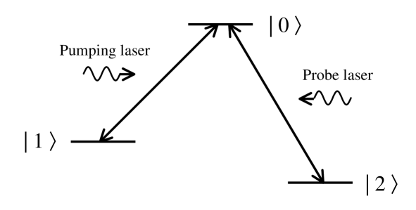
FIG. 1.: Energy diagram of a three-level $\Lambda$-type atom interacting with two laser beams, coupling the two ground states to a common excited atomic state.

The laser field coupled to the atomic transition between the states $|1\rangle$ and $|0\rangle$ will be called “pumping (or pump) laser”, and the laser coupled to the transition between the states $|2\rangle$ and $|0\rangle$ will be the “probe laser”. A typical experiment consists of scanning the frequency of the probe laser and measuring its transmitted intensity. In the absence of the pump laser, one observes a standard absorption resonance profile. Under certain conditions, the addition of the pump laser prevents absorption in a narrow portion of the resonance profile, and the transmitted intensity as a function of the probe frequency presents a narrow peak of induced transparency.

The effect depends strongly on the pump beam intensity. Typically the pump laser has to be intense so that the Rabi frequency $\Omega_{1}$ associated to the transition from state $|1\rangle$ to $|0\rangle$ is larger than all damping rates present (associated to spontaneous emission from the excited state and other relaxation processes). One of the effects of this pump beam is to induce an AC-Stark splitting of the excited atomic state. The probe beam will therefore couple state $|2\rangle$ to two states instead of one. If the splitting (which varies linearly with the Rabi frequency $\Omega_{1}$) is smaller than the excited state width, the two levels are indistinguishable and one expects quantum interference in the probe absorption spectrum. As the Rabi frequency $\Omega_{1}$ increases, the splitting becomes more pronounced and indistinguishability is lost. The absorption spectrum becomes a doublet called the Autler-Townes doublet. We will keep this image in mind to present a classical system with the same features.

A EIT-like phenomena with masses and springs

We will model our atom as a simple harmonic oscillator, consisting of a particle 1, of mass $m_{1}$, attached to two springs with spring constants $k_{1}$ and $K$ (see Fig. 2). The spring with constant $k_{1}$ is attached to a wall, while the other spring is attached to a second particle of mass $m_{2}$ and initially kept immobile at a fixed position. Particle 1 is also subject to a harmonic force ${\cal F}_{s}=Fe^{-i\ (\omega_{s}t+\phi_{s})}$. If we analyze the power transferred from the harmonic source to particle 1, as a function of frequency $\omega_{s}$, in this situation we will observe the standard resonance absorption profile discussed above (peaked at frequency $\omega_{1}^{2}=(k_{1}+K)/m$). If we now allow particle 2 to move, subject only to the forces from the spring of constant $K$ and a third spring of constant $k_{2}$, attached to a wall (see Fig. 2), this profile is modified. As we shall see, depending on the spring constant $K$, we can observe a profile presenting features similar to EIT evolving to an Autler-Townes-like doublet (as a matter of fact, this doublet is simply a normal-mode splitting). For simplicity, we will consider the situation in which $k_{1}=k_{2}=k$ and $m_{1}=m_{2}=m$.

The physical analogy between our model and the three-level atom coupled to two light fields is simple. As mentioned, the atom is modeled as oscillator 1 (particle 1), with its resonance frequency $\omega_{1}$. Since we chose $k_{1}=k_{2}=k$ and $m_{1}=m_{2}=m$, we have the analog of a degenerate $\Lambda$ system. The pump field is simulated by the coupling of oscillator 1 to a second oscillator via the spring of constant $K$ (reminding us of the quantized description of the field, in terms of harmonic oscillators). The probe field is then modeled by the harmonic force acting on particle 1.

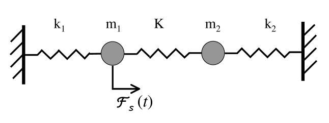
FIG. 2.: Mechanical model used to simulate EIT.

In order to provide a quantitative description of the system we write the equations of motion of particles 1 and 2 in terms of the displacements $x_{1}$ and $x_{2}$ from their respective equilibrium positions:

$$\ddot{x_{1}}(t)+\gamma_{1}\dot{x_{1}}(t)+\omega^{2}x_{1}(t)-\Omega_{r}^{2}x_{2}(t)=\frac{F}{m}e^{-i\ \omega_{s}t}$$ (1)

$$\ddot{x_{2}}(t)+\gamma_{2}\dot{x_{2}}(t)+\omega^{2}x_{2}(t)-\Omega_{r}^{2}x_{1}(t)=0\;,$$ (2)

where we set $\phi_{s}=0$ for the probe force without loss of generality. We also defined $\Omega_{r}^{2}=K/m$, the frequency associated with the coherent coupling between the pumping oscillator and the oscillator modeling the atom, $\gamma_{1}$ the friction constant associated to the energy dissipation rate acting on particle 1 (which simulates the spontaneous emission from the atomic excited state), and $\gamma_{2}$, the energy dissipation rate of the pumping transition.

Since, we are interested in the power absorbed by particle 1 from the probe force, we will seek a solution for $x_{1}(t)$. Let us suppose that $x_{1}(t)$ is of the form

$$x_{1}(t)=Ne^{-i\ \omega_{s}t}\;,$$ (3)

where $N$ is a constant. After taking a similar expression for $x_{2}(t)$ and substituting in eq. (2), we find

$$x_{1}(t)=\frac{(\omega^{2}-\omega_{s}^{2}-i\gamma_{2}\omega_{s})Fe^{-i\ \omega_{s}t}}{m[(\omega^{2}-\omega_{s}^{2}-i\gamma_{1}\omega_{s})(\omega^{2}-\omega_{s}^{2}-i\gamma_{2}\omega_{s})-\Omega_{r}^{4}]}\;.$$ (4)

Now, computing the mechanical power $P(t)$ absorbed by particle 1 from the probe force ${\cal F}_{s}$,

$$P(t)=Fe^{-i\ \omega_{s}t}\dot{x_{1}}(t)\;,$$ (5)

we find for the power absorbed during one period of oscillation of the probe force

$$P_{s}(\omega_{s})=-\frac{2\pi iF^{2}\omega_{s}(\omega^{2}-\omega_{s}^{2}-i\gamma_{2}\omega_{s})}{m[(\omega^{2}-\omega_{s}^{2}-i\gamma_{1}\omega_{s})(\omega^{2}-\omega_{s}^{2}-i\gamma_{2}\omega_{s})-\Omega_{r}^{4}]}\;.$$ (6)

In Fig. 3 we show the real part of $P_{s}(\omega_{s})$, for six different values of the coupling frequency $\Omega_{r}$ expressed in frequency units. These curves were obtained using the values $\gamma_{1}=0.1\times 10^{-6}$, $\gamma_{2}=0.4\times 10^{-1}$, and $\omega_{0}=\sqrt{k/m}=2.0$, all expressed in the same frequency units. The amplitude $F/m$ was taken equal to $0.1$ force per mass units.

For $\Omega_{r}=0$ we have a typical absorption profile, with a maximum probe power absorption for $\delta=0$, being $\delta$ the detuning between the probe and the oscillator frequencies ($\delta=\omega_{s}-\omega$). Incrementing the value of $\Omega_{r}$ to 0.1, we observe the appearance of a narrow dip in the absorption profile of the probe power. This zero absorption at the center frequency of the profile is an evidence of a destructive interference between the normal modes of oscillation of the system [8]. A further increment of the coupling frequency leads to the apparition of two peaks in the probe power absorption profile, that are clearly separated for $\Omega_{r}=0.5$. This effect in atomic systems is called the AC-Stark splitting or Autler-Townes doublet.

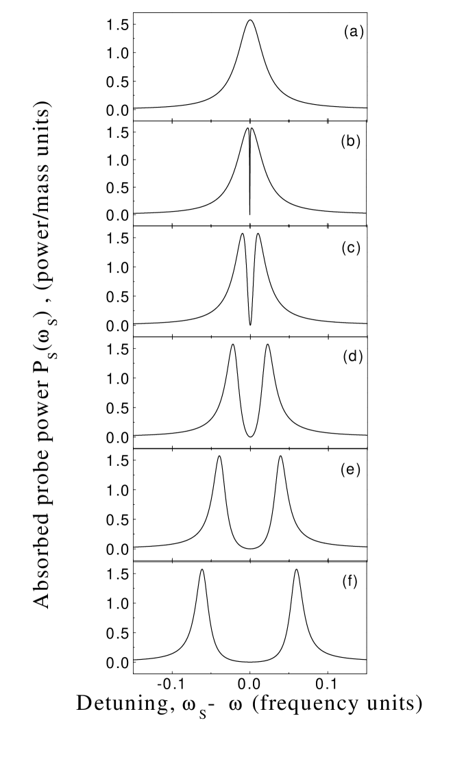
FIG. 3.: Frequency dependence of the absorption of the probe energy by particle 1. The values of $\Omega_{r}$ in each case are (a) 0.0 , (b) 0.1 , (c) 0.2 , (d) 0.3 , (e) 0.4 , and (f) 0.5 , all expressed in frequency units.

An important fact to be pointed out is that the dissipation rate $\gamma_{2}$, associated to the energy loss of the pumping oscillator, must be much smaller than $\gamma_{1}$ in order to achieve a regime of coherent driving of particle 1’s oscillation. In other words, there should be no significant increase of dissipation in the system by adding the pumping oscillator. In the case of EIT [9], the condition analogous to $\gamma_{2}\ll\gamma_{1}$ is that the transfer rate of population from the atomic ground state $|1\rangle$ to $|2\rangle$ should be negligible (see Fig. 1). In both situations, the violation of this condition obstructs the observation of the induced transparency.

Another important result reproduced with this mechanical model is the dispersive behavior of the mass oscillator used to simulate the atom. The dispersive response is contained in the real part of the frequency dependence of the amplitude of oscillation $x_{1}(t)$ of particle 1, given by eq. (4). In Fig. 4 we plot this quantity for $\Omega_{r}=0.1$. This value of $\Omega_{r}$ corresponds to the situation when the induced transparency is more pronounced and, as we can see from Fig. 4, the dispersion observed, in the frequency interval where we have the induced transparency, is normal and with a very steep slope.

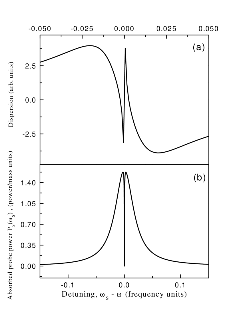
FIG. 4.: Dispersive (a) and absorptive (b) responses of the probe power transferred to particle 1, for $\Omega_{r}=0.1$ frequency units.

This result coincides with that reported before in an experimental realization of electromagnetically induced transparency [10]. It is also important to point out that this very steep normal dispersion is responsible for the recently observed slow propagation of light (slow light) [2, 3, 4], and the “freezing” of a light pulse in an atomic medium [5, 6]. It should therefore be possible to observe such propagation effects considering absorption in a medium consisting of a series of mechanical ‘atom-analogs’.

This theoretical model is not the only classical one to simulate EIT-like phenomena. As mentioned, in this model the pump field is replaced by a harmonic oscillator, simulating a quantum-mechanical description. In most theoretical descriptions of EIT in atomic media, pump and probe fields are classical. The mechanical analog to this description would then involve only one oscillator (one particle of mass $m$). In this analysis, it becomes apparent that EIT arises directly from a destructive interference between the oscillatory forces driving the particle’s movement. In order to keep the text simple, we have chosen to not present this description here. Furthermore, it is not related to the experimental results presented below.

III EIT-like phenomena in coupled $RLC$ circuits: a simple undergraduate laboratory experiment

An experiment to observe the predictions of the previous section, although possible, would not be straightforward. Instead, we decided to use the well-known analogy between mechanical oscillators and electric circuits to perform a simple experiment. The electric analog to the system of Fig. 2, is the circuit shown in Fig. 5, where the circuit mesh composed by the inductor $L_{1}$ and the capacitors $C_{1}$ and $C$ simulates the pumping oscillator, and the resistor $R_{1}$ determines the losses associated with that oscillator. The atom is modeled using the resonant circuit formed by the inductor $L_{2}$, the capacitors $C_{2}$ and $C$, and the resistor $R_{2}$ represents the spontaneous radiative decay from the excited level. The capacitor $C$, belonging to both circuit meshes, models the coupling between the atom and the pumping field, and determines the Rabi frequency associated to the pumping transition. In this case, the probe field is simulated by the frequency-tunable voltage source $V_{S}$.

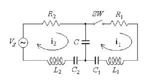
FIG. 5.: Electric circuit employed to investigate the induced transparency.

The circuit mesh used to model the atom has only one resonance frequency representing the energy of the atomic excited level. That is to say, the probability of excitation of this circuit will be maximal when the applied harmonic force is on resonance. Since in this case we have two possible paths to accomplish this excitation, we are dealing with the analog of a three-level atom in the $\Lambda$ configuration. Namely, the oscillator corresponding to the ‘atom-analog’ can be excited directly by the applied voltage $V_{s}$ or by the coupling to the pumping oscillator.

Here again the induced transparency is investigated analyzing the frequency dependence of the power $P_{2}(\omega_{s})$ transferred from the voltage source $V_{S}$ to the resonant circuit $R_{2}L_{2}C_{e2}$,

$$P_{2}(\omega_{s})=\Re\{{\cal V}_{S}{\cal I}_{2}^{*}\}\;,$$ (7)

where ${\cal V}_{S}$ and ${\cal I}_{2}$ are respectively the complex representations of $V_{S}$ and $i_{2}(t)$, and the equivalent capacitor $C_{e2}$ is the series combination of $C$ and $C_{2}$:

$$C_{e2}=\frac{CC_{2}}{C+C_{2}}\;.$$ (8)

Setting $L_{1}=L_{2}=L$ ($m_{1}=m_{2}=m$ in the mechanical model) and writing the equations for the currents $i_{1}(t)=\dot{q_{1}}(t)$ and $i_{2}(t)=\dot{q_{2}}(t)$ shown in Fig. 5, we find the following system of coupled differential equations for the charges $q_{1}(t)$ and $q_{2}(t)$:

$$\ddot{q_{1}}(t)+\gamma_{1}\dot{q_{1}}(t)+\omega_{1}^{2}q_{1}(t)-\Omega_{r}^{2}q_{2}(t)=0$$ (9)

$$\ddot{q_{2}}(t)+\gamma_{2}\dot{q_{2}}(t)+\omega_{2}^{2}q_{2}(t)-\Omega_{r}^{2}q_{1}(t)=\frac{V_{S}(t)}{L_{2}}\;.$$ (10)

Here $\gamma_{i}=R_{i}/L_{i}$ ($i=1,2$), $\omega_{i}^{2}=1/(L_{i}C_{ei})$, and $\Omega_{r}^{2}=1/(L_{2}C)$. These equations coincide with the eqs. (2) using the correspondences shown in Table 1 and $\omega_{1}=\omega_{2}$. Therefore, both models describe the same physics.

Mechanical model	Electrical model
$\gamma_{1}$ ($\gamma_{2}$)	$R_{1}/L_{1}$ ($R_{2}/L_{2}$)
$m_{1}$ ($m_{2}$)	$L_{1}$ ($L_{2}$)
$k_{1}$ ($k_{2}$)	$1/C_{1}$ ($1/C_{2}$)
$K$	$1/C$
$x_{1}$ ($x_{2}$)	$q_{1}$ ($q_{2}$)
$(F/m)\,e^{-i\ \omega_{s}t}$	${\cal V}_{S}(t)/L_{2}$

TABLE I.: Correspondences between the mechanical and electrical parameters.

Once the current $i_{2}(t)$ (or ${\cal I}_{2}$) is known, the expression that determines the power $P_{2}(\omega_{s})$ as a function of the frequency $\omega_{s}$ of the applied voltage, when the switch $SW$ in Fig. 5 is closed, is given by

$$P_{2}(\omega_{s})=\frac{p1(\omega_{s})}{p1(\omega_{s})^{2}+p2(\omega_{s})^{2}}|A_{S}|^{2}\;,$$ (11)

where

$$p1(\omega_{s})=R_{2}+\frac{R_{1}/(\omega_{s}C)^{2}}{R_{1}^{2}+(\omega_{s}L_{1}-1/(\omega_{s}C_{e1}))^{2}}$$ (12)

$$p2(\omega_{s}) = (\omega_{s}L_{2}-1/(\omega_{s}C_{e2}))-$$ (14)

$$\frac{(1/(\omega_{s}C)^{2})(\omega_{s}L_{1}-1/(\omega_{s}C_{e1}))}{R_{1}^{2}+(\omega_{s}L_{1}-1/(\omega_{s}C_{e1}))^{2}}\;,$$

being $C_{e1}$ the equivalent capacitor given by the series combination of $C$ and $C_{1}$ and $A_{S}$ represents the amplitude of the applied voltage. On the other hand, when the switch is open we have

$$P_{2}(\omega_{s})=\frac{R_{2}}{R_{2}^{2}+(\omega_{s}L_{2}-1/(\omega_{s}C_{e2}))^{2}}|A_{S}|^{2}\;.$$ (15)

There are many ways of measuring the power $P_{2}(\omega_{s})$. We have chosen to measure the current flowing through the inductor $L_{2}$, which has the same frequency dependence as $P_{2}(\omega_{s})$. We actually measure the voltage drop across the inductor $L_{2}$ and integrate it to find a voltage proportional to the current flowing through the inductor. This voltage is an oscillatory signal at the frequency $\omega_{s}$. We are interested in the amplitude of this signal, which we read off an oscilloscope.

In Fig. 6 are presented the experimental amplitudes measured, corresponding to four different values of the coupling capacitor $C$. For each value of the coupling capacitor a measurement was made in two situations: with the switch open (open square) and with the switch closed (open circle). In Table 2 we present the specifications of the electronic components used in the experiment.

Electronic component	Value
$R_{1}$	$0$ Ohms
$R_{2}$	$51.7$ Ohms
$L_{1}$	$1000$ $\mu$ H
$L_{2}$	$1000$ $\mu$ H
$C_{1}$	$0.1$ $\mu$ F
$C_{2}$	$0.1$ $\mu$ F

TABLE II.: Specifications of the electronic components used in the experiment.

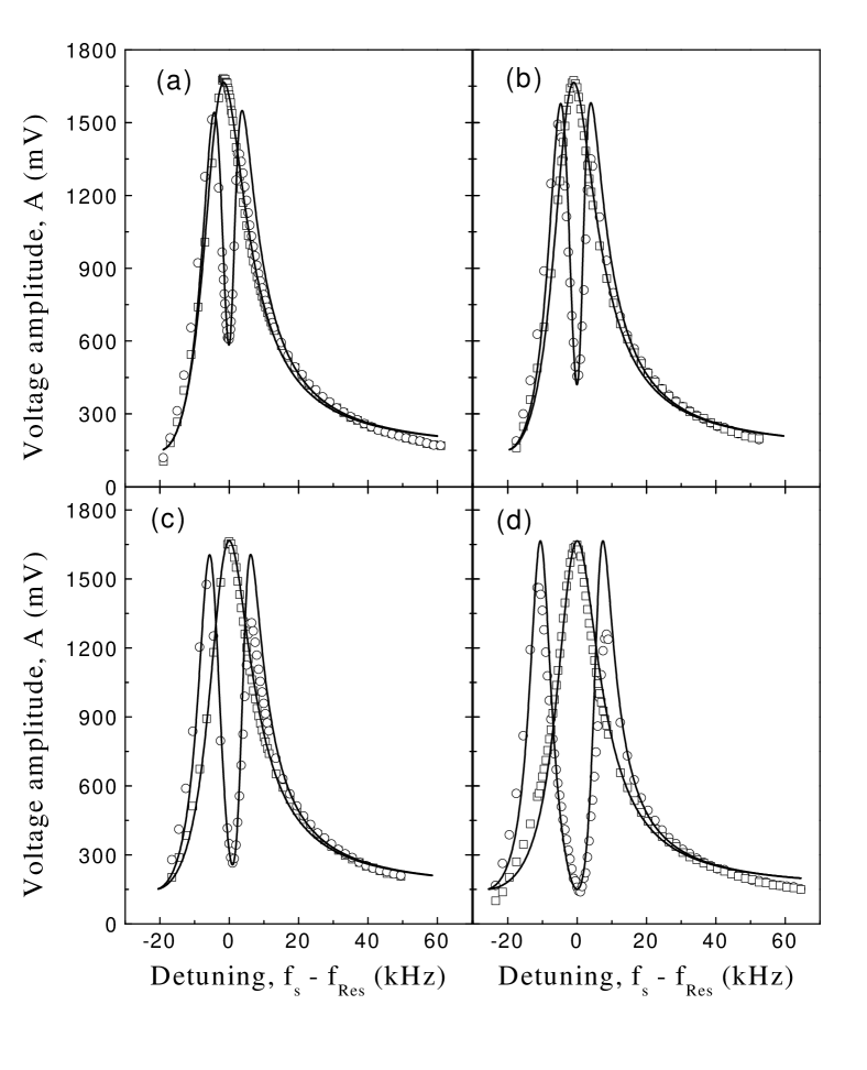
FIG. 6.: Power transferred to the circuit $R_{2}L_{2}C_{e2}$ as a function of the frequency $\omega_{s}$ for different values of the coupling capacitor $C$. The values of $C$ in each curve are (a) $C=0.196\mu$ F, with resonance frequency f${}_{\mbox{Res}}=\omega_{2}/2\pi=20.0$ kHz, (b) $C=0.150\mu$ F, f${}_{\mbox{Res}}=19.5$ kHz, (c) $C=0.096\mu$ F, f${}_{\mbox{Res}}=21.5$ kHz, (d) $C=0.050\mu$ F, f${}_{\mbox{Res}}=26.5$ kHz. The open squares correspond to measurements made with the switch $SW$ open (see Fig. 5), which is equivalent to turning the pump off. The open circles correspond to measurements made with the switch closed. The solid curves are a comparison to the theory presented in § III. The evolution from EIT to the Autler-Townes regime is clearly observed.

As we can see from Fig. 6, in the open switch configuration (no pumping) we have a maximum coupling of electrical power from the voltage source $V_{S}$ to the resonant circuit $R_{2}L_{2}C_{e2}$ at the resonant frequency (zero detuning). When the switch is closed, that is to say, the pumping circuit (pumping force) is acting on the resonant circuit $R_{2}L_{2}C_{e2}$, we have a depression of the absorption of the electrical power of the voltage source at zero detuning. This fact corresponds to the transparent condition, and is more pronounced when the value of the coupling capacitor is reduced, corresponding to an increment of the Rabi frequency of the pumping field in electromagnetically induced transparency studied in atomic systems.

Here, as in the experiments with atoms and light, the observed transparency can be interpreted as a destructive interference. In this case, the inteference is between the power given by the voltage source to the resonant circuit $R_{2}L_{2}C_{e2}$, and the power transferred to the same circuit from the other oscillator representing the pumpimg force. As explained in §II A, it can also be viewed as an interference between the two possible excitation paths corresponding to the normal modes of the coupled oscillators. For the minimum value of $C$ used in our experiment (see Fig. 6(d)), we observe two absorption peaks, as the classical analog of the Autler-Townes effect or AC-Stark splitting, which correspond to the splitting of these normal modes. We should also point out that the smallest coupling value we used (Fig. 6(a)) did not lead to an infinitely narrow transparency peak as would be expected from the value $R_{1}=0$. This is probably due to internal “residual” series resistances of the components we used.

The solid lines shown in Fig. 6 represent the theoretical results obtained using eqs. (11) or (15). These curves are not intended to fit exactly the experimental data since our measurements are affected by the frequency response of the integrator used to derive the voltage proportional to the current in the inductor $L_{2}$. It is not our purpose to analyze in detail the deviations of our system from the ideal model proposed.

It is also possible to measure the dispersive response of our ‘atom-analog’. One has to analyze the relative phase between the oscillating current flowing through inductor $L_{2}$ and the phase of the applied voltage. This measurement is best if performed with a lock-in amplifier. Since this equipment is not usually available in undergraduate laboratories, we prefer to describe a simple procedure which does not lead to a real measurement to be compared with the theoretical prediction (Fig. 4). We observe the oscillatory signal on the oscilloscope corresponding to the current flowing through the inductor, with the trigger signal from the voltage source $V_{S}(t)$. The phase of the sinusoidal signal is observed to “jump” as we scan $\omega_{s}$ across the absorption resonance and transparency region. If we scan $\omega_{s}$ increasing its value, we observe three abrupt phase variations, with the intermediate one being opposite to the other two. This is exactly what we would expect from Fig. 4.

IV Conclusion

We have shown that EIT can be modeled in a totally classical system. Our results extend the results of Hemmer and Prentiss [7] to EIT-like phenomena, with the use of only two coupled oscillators instead of three. We also deal with the dispersive response of the classical oscillator used to model the three-level atom. We performed an experiment with coupled $RLC$ circuits and observed EIT-like signals and the classical analog of the Autler-Townes doublet as a function of the coupling between the two $RLC$ circuits. The experiment can be performed in undergraduate physics laboratories and should help form physical intuition on coherent phenomena which take place in atomic vapors.

REFERENCES

- [1] See, for example, S. E. Harris, “Electromagnetically Induced Transparency”, Phys. Today 50 (7), 36-42 (1997).
- [2] L. V. Hau, S. E. Harris, Z. Dutton, and C. H. Behroozi, “Light speed reduction to 17 metres per second in an ultracold atomic gas”, Nature 397, 594-598 (1999).
- [3] M. M. Kash, V. A. Sautenko, A. S. Zibrov, L. Hollberg, G. R. Welch M. D. Lukin, Y. Rostovtsev, E. S. Fry, and M. O. Scully, “Ultraslow Group Velocity and Enhanced Nonlinear Optical Effects in a Coherently Driven Hot Atomic Gas”, Phys. Rev. Lett. 82, 5229-5232 (1999).
- [4] D. Budker, D. F. Kimball, S. M. Rochester, and V. V. Yashchuk, “Nonlinear Magneto-optics and Reduced Group Velocity of Light in Atomic Vapor with Slow Ground State Relaxation”, Phys. Rev. Lett. 83, 1767-1770 (1999).
- [5] C. Liu, Z. Dutton, C. H. Behroozi, and L. V. Hau, “Observation of coherent optical information storage in an atomic medium using halted light pulses”, Nature 409, 490-493 (2001).
- [6] D. F. Phillips, A. Fleischhauer, A. Mair, R. L. Walsworth, and M. D. Lukin, “Storage of Light in Atomic Vapor”, Phys. Rev. Lett. 86, 783-786 (2001).
- [7] P. R. Hemmer and M. G. Prentiss, “Coupled-pendulum model of the stimulated resonance Raman effect”, J. Opt. Soc. Am. B 5, 1613-1623 (1988).
- [8] As explained, the induced transparency results from the existence of two possible paths for the absorption of the probe energy to excite the oscillation of particle 1. We can see these paths in eq. (6) rewriting it as a superposition of the normal modes of oscillation of the coupled oscillators.
- [9] Y.-q. Li, and M. Xiao. “Observation of quantum interference between dressed states in an electromagnetically induced transparency”, Phys. Rev. A 51, 4959-4962 (1995).
- [10] M. Xiao, Y.-q. Li, S.-z. Jin, and J. Gea-Banacloche, “Measurement of Dispersive Properties of Electromagnetically Induced Transparency in Rubidium Atoms”, Phys. Rev. Lett. 74, 666-669 (1995).