Fuzziness in Quantum Mechanics

Abstract

It is shown that quantum mechanics can be regarded as what one might call a ”fuzzy” mechanics whose underlying logic is the fuzzy one, in contradistinction to the classical ”crisp” logic. Therefore classical mechanics can be viewed as a crisp limit of a ”fuzzy” quantum mechanics. Based on these considerations it is possible to arrive at the Schroedinger equation directly from the Hamilton-Jacobi equation. The link between these equations is based on the fact that a unique ( ”crisp”) trajectory of a classical particle emerges out of a continuum of possible paths collapsing to a single trajectory according to the principle of least action. This can be interpreted as a consequence of an assumption that a quantum ”particle” ”resides” in every path of the continuum of paths which collapse to a single( unique) trajectory of an observed classical motion. A wave function then is treated as a function describing a deterministic entity having a fuzzy character. As a consequence of such an interpretation, the complimentarity principle and wave-particle duality can be abandoned in favor of a fuzzy deterministic microoobject.

1 Introduction

One of the purposes of this paper is to bring together fuzzy logic and quantum mechanics. Here we extend our prior analysis [1] of a fuzzy logic interpretation of quantum mechanics by demonstrating that the Schroedinger equation can be deduced from the assumptions of the fuzziness underlying not only quantum but also classical mechanics. A pedestrian way of defining fuzziness was given by Kosko [2] who wrote that the fuzzy principle states that everything is a matter of degree. More rigorously, fuzziness can be defined as multivalence.

Interestingly enough, even separation between classical and quantum domains is somewhat fuzzy since there is no crisp boundary separating them ( see, for example, [3]). Moreover, we can even claim that the difference between these domains is only in a degree of fuzziness. In fact, both classical and quantum mechanics make predictions based on repetitive measurements which imply a certain spread of results.

The crisp character of the formal apparatus of classical mechanics hides this important fact by a seemingly absolute character of a single measurement. From this point of view the ultimate statements of classical mechanics are nothing but the results a certain averaging ( or defuzzification, meaning the elimination of the spread) with some weight which we call the ”fuzziness density”. The latter can be represented by some function. The fuzziness density then varies from ”sharp’ ( in classical mechanics) to ”diffuse” (in quantum mechanics).

If we consider a concept of a ”thing in itself” and assume(quite plausibly) that it has a fuzzy and deterministic character, then in a series of experiments designed to elicit its properties to the outside observers it appears as a random set thus disguising its deterministic nature. As we have already indicated, we consider classical and quantum mechanics as having common fuzzy roots and no sharp dividing boundary. They can be viewed as different realizations of a fuzzy ”thing in itself”. This can explain why some phenomena in a strongly fuzzy domain of quantum mechanics cannot be realized in a weakly fuzzy (more precisely, zero fuzzy) domain of classical mechanics.

Thus if we accept quantum mechanics as a more general theory than classical mechanics, then it seems reasonable to expect that the former could be constructed independently from the latter. However the basic postulates of quantum mechanics cannot be formulated , even in principle, without invoking some concepts of classical mechanics. Both theories share some basic common feature, namely that they are rooted in the fuzzy reality. This somehow justifies a paradoxical statement by Goldstein (as quoted in [4]) that quantum mechanics is a repetition of classical mechanics suitably understood.

Our basic assumption is that reality is fuzzy and nonlocal not only in space but also in time. In this sense idealized pointlike particles of classical mechanics corresponding to the ultimate ”sharpness” of the fuzziness density emerge in a process of interaction between different parts of fuzzy wholeness. This process is viewed as a continuous process of defuzzification. It transforms a fuzzy reality into a crisp one. It is clear that the emerging crisp reality (understood as a final step of measurements which we call detection) carries less information that the underlying fuzzy reality. This means that there is an irreversible loss loss of information usually called a collapse of the wave function within a context of quantum mechanics. From our point of view it is not so much a ”collapse’ as a realization of one of many possibilities existing within a fuzzy reality. Any measurements (viewed as a process) rearranges the fuzzy reality leading to different detection outcomes according to the changed fuzziness.

Therefore it seems quite reasonable to expect that classical theory bears some traces of quantum theory underlying (and connected to)it. In view of this we would like to recall the words by Bridgeman who remarked that the seeds and the sources of the ineptness of our thinking in the microscopic range are already contained in our present thinking applied to a large-scale regions. One should have been capable of discovery of the former by a sufficiently critical analysis of our ordinary common sense thinking.

2 Some Basic Concepts

As we have already indicated, both classical and quantum mechanics can be viewed as statistical theories (cf. [5])with respect to an ensemble of repetitive measurements where each measurement must be carried out under the identical conditions. The latter is a very restrictive requirement dictated by a crisp-logical world view and therefore not attainable even in a more general setting of fuzzy reality. On the other hand, if we assume a fuzzy nature of ”things” then the apparent statistical character of physical phenomena would follow not from their intrinsic randomness but from their fuzzy-deterministic nature. Outwardly the latter expresses itself as randomness. Clearly, this definition of the apparent statistical nature of classical and quantum mechanics is applicable even to one measurement.

Let us elaborate on this.Conventionally, statistical theories are tied to randomness. However recent results in the theory of fuzzy logic provided a deterministic definition of the relative frequency count of identical outcomes by expressing it as a measure of a subsethood $S(A,B)$, that is a degree to which a set $A$ is a subset of a set $B$ [6]. To make it more concrete suppose that set $B$ contains $N$ trials and set $A$ contains $N_{A}$ $\it succesful$ trials. Then $S(A,B)=N_{A}/N$.

We would like to extend this concept to experimental outcomes of measurements performed on a classical particle. This would be possible if we were to to consider the classical particle to be located simultaneously on all possible paths connecting two spatial points. In a sense it is not so far fetched since it is analogous to the idea used by the least action principle.

To adapt the concept of fuzziness to a spatial localization of a particle we introduce the notion of the particle’s membership in a spatial interval ( one-, two, or three-dimensional). This membership, generally speaking, is going to vary from one interval to another. We define the membership as follows. Let us say that we perform $N$ measurements aimed at detecting the particle in a certain spatial interval. It turns out that the particle is found in this interval $N_{A}$ times. The membership of the particle in the interval is then defined as $N_{A}/N$ and can be formally described with the help of Zadeh [7] sigma-function.

As a next step, this approach allows us to formally introduce the membership  density defined as the derivative of the membership function. If we denote the membership density by $\mu$, then a degree of membership of the particle say in an elemental volume $\Delta V$ is $\mu\Delta V$. According to this definition the particle has a $zero$ membership in a spatial interval of measure $0$, that is at a point. Such an apparently paradoxical result indicates that in general we should base our estimation of fuzziness on the relative degree of membership instead of the absolute one.

In other words, given a degree of membership $\mu(x_{i})dV$ of a particle in a volume $dV$ containing the point $x_{i}$ and a degree of membership $\mu(x_{j})dV$ of the same particle in a volume $dV$ containing the point $x_{j}$, we find the $relative~{}~{}degree$ of membership of the particle in both volumes: $\mu(x_{i})/\mu(x_{j})$. The same expression represents also the relative degree of membership of the particle in two points $x_{i}$ and $x_{j}$ despite the fact that the absolute degree of membership of the particle in either point is $0$.

An importance of the relative degree of membership is due to the fact that experimentally a location of the particle is evaluated on the basis of its detection at a certain location in $N_{i}$ experimental trials out of $N$ trials. As was shown by Kosko [6], the ratio $N_{i}/N$ then measures the degree to which a sample of all elementary outcomes of the experiments is a subset of a space of the successful outcomes. In other words, this ratio represents a degree of membership of the sample space in the space of the successful outcomes. In our case the relative degree of membership $\mu(x_{i})/\mu(x_{j})$ of a particle in two points can be identified as the relative count of the successful outcomes (in a series of measurements) of finding the particle at points $x_{i}$ and $x_{j}$.

In view of these definitions the classical mechanical sigma-curve of particle’s membership in a spatial interval is nothing but a step function. This simply means that up to a certain spatial point $x$ the degree of particle’s membership in an interval ($-\infty,x]$ is $0$, and for any value $y>x$ the degree of particle’s membership in the interval ($x,y]$ is $1$. The corresponding membership density is the delta function. Thus the idealized picture of classical-mechanical phenomena with particles occupying intervals of measure zero corresponds to the statement that these particles are $\it strictly$ non-fuzzy , their behavior is governed by a crisp bivalent logic, and the respective membership density is the delta-function.

In reality, any physical ”particle” occupies a small but nonzero spatial interval. This means that the membership density is a sharp ( but not delta-like) function corresponding to a minimum fuzziness. At the other end of the spectrum, in the microworld, the fuzziness is maximal. In fact, if we accept the idea that a quantum mechanical ”particle” (a microobject) ”resides” in different elemental volumes $dV$ of a three-dimensional space with the varying degrees of residence (membership), then we can apply to such a microobject our concept of the membership density. In general, this density cannot be made arbitrarily narrow as is the case for a classical particle. The latter can be considered as the limiting case of the former when the membership density becomes delta-function-like. Moreover, the fuzziness in the microworld is even more subtle since mathematically it is described with the help of complex-valued functions.

The latter results in the emergence of the interference phenomenon for microobjects, which in the classical domain is an exclusive property of waves. Therefore, mutually exclusive concepts of particles and waves in classical mechanics become inapplicable in the realm of fuzzy reality where ”particles” and ”waves” are not mutually exclusive concepts, but rather different expressions of fuzziness. For example, the double-slit experiment can be interpreted now as a microobject’s ”interference with itself” because it has a simultaneous membership in all parts of space including elemental volumes containing both slits. Since the total membership of a microobject in a given finite volume is fixed, any change of its membership in one of the slits affects the membership everywhere leading to the interference effects.

In the following we ”recover” the fuzziness of the quantum world by deriving the Schroedinger equation from the Hamilton-Jacobi equation, where the latter can be viewed as the result of the fuzziness reduction ( destruction) of the quantum world.

3 DERIVATION OF THE SCHROEDINGER EQUATION

First, we show how the Hamilton-Jacobi equation for a classical particle in a conservative field can be derived from Newton’s second law, thus connecting it to the destruction of fuzziness. In principle, a particle’s motion between two fixed points, A and B, can occur along any conceivable path (a ”fuzzy” ensemble in a sense that a particle has membership in each of the paths) connecting these two points. In the observable reality these paths ”collapse” onto one observable path. Mathematically, this reduction is achieved by imposing a certain restriction on a certain global quantity (the action $S$), defined on the above family of paths.

Let us consider Newton’s second law and assume that trajectories connecting points $A$ and $B$ comprise a continuous set. This means in particular that the classical velocity is now a function of both the time and space coordinates, $\bf v=\bf v(\bf x$,$t)$. Now we fix time $t=t_{0}$. Since on the above set for the fixed $t_{0}$ the correspondence $\bf x$ to $t$ is many to one, $\bf x$ is not fixed (as was the case for a single trajectory), and therefore the velocity would vary with $\bf x$. Physically this is equivalent to considering points on different trajectories at the same time. Our assumption means that now we must use the total time derivative:

$$d/dt=\partial/\partial t+\bf V\bullet\bf\nabla$$ (1)

By applying the curl operation to Newton’s second law for a single particle and performing elementary vector operations we obtain

$$(\partial/\partial t){\bf\nabla\times p}-(1/m){\bf\nabla\times(p\times\nabla\times p)}=0,$$ (2)

where $p=m{\bf v}$ is the particle’s momentum. If we view (2) as the equation with respect to $\bf{\nabla}\times\bf{p}$, then one of its solutions is

$$\bf{p}=\nabla S$$ (3)

where $S(\bf{x},t)$ is some scalar function to be found. Since $S$ is defined on the continuum of paths it can serve as a function related to the notion of fuzziness (here a continuum of possible paths).

Note that the spatial and time variables enter into $S$ on equal footing. Upon substitution of (2) back in Newton’s second law, $d\bf{p}/dt=-\nabla V$, where $d/dt$ is understood in the sense of (1), we obtain

$$\nabla[\partial S/\partial t+(l/2m)(\nabla S)^{2}+V]=0$$

.

Integrating this equation and incorporating the constant of integration (which, generally speaking, is some function of time) into the function $S$, we arrive at the determining equation for the function $S$ which is the familiar Hamilton-Jacobi equation for a classical particle in a potential field $V$:

$$\partial S/\partial t+(l/2m)(\nabla S)^{2}+V=0.$$ (4)

By using Eqs. (1) and (3) we can represent $S$ as a functional defined on the continuum of paths connecting two given points, say $0$ and $1$, corresponding to the moments of time $t_{0}$ and $t_{1}$. To this end we rewrite (4):

$$dS/dt=p^{2}/2m+V$$ (5)

Integrating (5) we obtain the explicit expression of $S$ in the form of the following functional:

$$S=\int_{t_{0}}^{t_{1}}(\frac{p^{2}}{2m}-V)dt,$$ (6)

which is the well-known definition of the action for a particle moving in the potential field $V$. Thus we have connected the concept of fuzziness in classical mechanics with the action $S$. If we consider $S$ as a measure of fuzziness in accordance with our previous discussion, then by minimizing this functional (i.e., by postulating the principle of least action) we ”eliminate” (or rather minimize) fuzziness by generating the unique trajectory of a classical particle. In a certain sense the principle of least action serves as a defuzzification procedure.

Now we proceed with the derivation of the Schroedinger equation. There are two basic experimental facts that make microobjects so different from classical particles. First, all the microscale phenomena are linear. Second (which is a corollary of the first), these phenomena obey the superposition principle. Here it would be useful to recall that even at the initial stages of development of quantum mechanics Dirac formulated its fuzzy character, albeit without using the modern-day terminology. He wrote: ” … whenever the system is definitely in one state we can consider it as being partly in each of two or more other states”[8]. This is as close as one can come to the concepts of fuzzy sets and subsethood [9] without directly formulating them. In view of this it does not seem strange that a microobject sometimes can exhibit wave properties. On the contrary, they arise quite naturally as soon as we accept the fuzzy basis (meaning ”being partly in…other states”) of microscale phenomena which implies, among other things, the above-mentioned ”self-interference.”

How can we derive the equation that would incorporate these essential features of microscale phenomena and, under certain conditions, would yield the Hamilton-Jacobi equation of classical mechanics? We start with the Hamilton-Jacobi equation (not Newton’s second law) because of its connection to the hidden fuzziness in classical mechanics. We consider the simplest classical object that would allow us to get the desired results that will account for the two experimental facts mentioned earlier.

We choose a free particle by setting $V=0$ in Eq. (4). Our problem is somewhat simplified now. We are looking for a linear equation whose wave-like solution is simultaneously a solution of the Hamilton-Jacobi equation. Since the mechanical phenomena behave differently at microscales and macroscales, the linear equation should contain a scale factor (that is to be scale-dependent), such that in the limiting case corresponding to the macroscopic value of this factor we get the nonlinear Hamilton-Jacobi equation for a free particle.

A nonlinear equation admits a wave-like solution (for a complex wave) if this equation is homogeneous of order $2$. Since Eq. (4) does not satisfy this criterion, we cannot expect to find a wave solution for the function $S$. However, this turns out to be a blessing in disguise, because by employing a new variable in place of the action $S$, we can both convert this equation into a homogeneous (of order 2) equation (thus allowing for a wave-like solution) and simultaneously introduce the scaling factor. It is easy to show that there is one and only one transformation of variables that would satisfy both conditions:

$$S=Kln\Psi$$ (7)

where the scaling factor $K$ is to be found later.

Upon substitution of (7) in (4), with $V=0$, we obtain the following homogeneous equation of the second order with respect to the new function $\Psi$:

$$K\Psi\frac{\partial\Psi}{\partial t}+\frac{K^{2}}{2m}(\nabla\Psi)^{2}$$ (8)

Equation (8) is easily solved by the separation of variables, yielding

$$\Psi=Cexp[-\frac{{at-(2m/a)^{1/2}\bf{a\bullet x}}}{K}]$$ (9)

where the vector $\bf{a}$ of length $a$ is another constant of integration. Since solution (9) must be a complex-valued wave, the argument of $\Psi$ must satisfy two conditions:

i)it must be imaginary, and

ii)the factors at the variables $t$ and $\bf{x}$ must be the frequency $\omega=2\pi\nu$ and the wave vector $\bf{k}$, respectively.

This results in the following:

$$K=-iB$$ (10)

and

$$a/B=\omega,~{}~{}(2m/a)^{1/2}\bf{a/B}=\bf{k}$$ (11)

where $B$ is a real-valued constant. Now the solution (9) is

$$\Psi=Cexp[-i(\omega t-\bf{k\bullet x}]$$ (12)

Since both functions $S$ and $\Psi$ are related by Eq. (7), we can easily establish the connection between the kinematics parameters of the particle and the respective parameters $\omega$ and $\bf{k}$, which determine the wave-like solution of the Hamilton-Jacobi equation for the new variable $\Psi$. According to classical mechanics, $-\partial S/\partial t$ is the particle energy $E_{0}$, and $\nabla S$ is the particle momentum $\bf{p}$. On the other hand, these quantities can be expressed in terms of the new variable $\Psi$ with the help of Eqs. (7) and (12), yielding $E_{0}=B\omega,B\bf{k}=\bf{p}$.

From these relations we see that for a free particle its energy (momentum) is proportional to the frequency $\omega$ (wave vector k ) of the wave solution to the ”scale-sensitive” modification of the Hamilton-Jacobi equation. The constant $B$ is found by invoking the experimental fact that $E_{0}=h\nu=\hbar\omega$ (where $h$ is Planck’s constant). This implies $B=\hbar$ or $K=-i\hbar$, and as a byproduct, the de Broglie equation ${\bf{p}}=\hbar\bf{k}$. Inserting solution (12) into the original nonlinear equation (8), we arrive at the dispersion relation

$$\omega=(\hbar/2m)k^{2}$$ (13)

Now we can find the linear wave equation whose solution and the resulting dispersion relation are given by Eqs.(12) and (13) respectively. Using an elementary vector identity, we rewrite Eq. (8):

$$[\frac{\partial}{\partial t}-\frac{i\hbar}{2m}{\nabla}^{2}]\Psi-\frac{i\hbar}{2m\Psi}[div(\Psi\nabla\Psi)-2\Psi{\nabla}^{2}\Psi]=0$$ (14)

Equation (14) is the sum of the two parts, one linear and the other nonlinear in $\Psi$. The solution (12) makes the nonlinear part identically zero, and this solution, together with the dispersion relation (13), must also satisfy the linear part of Eq. (14). Therefore we have proven the following: If the wave-like solution (12) satisfies Eq. (8), then it is necessary and sufficient that it must be a solution of the following linear partial differential equation, the Schroedinger equation:

$$[i\hbar\frac{\partial}{\partial t}+\frac{{\hbar}^{2}}{2m}{\nabla}^{2}]\Psi=0$$ (15)

Now we return to the variable $S$ according to $\Psi=exp(iS/\hbar)$ and introduce the following dimensionless quantities: time $\tau=t/t_{0}$, spatial coordinates ${\bf{R}}={\bf{x}}/L_{0}$ , the parameter ${\bf{h}}=\hbar/S_{0}$ (which we call the Schroedinger number), and the dimensionless action ${\bf{S}}=S/S_{0}$. Here, $S_{0}=mL^{2}_{0}/t_{0}$, $L_{0}$ is the characteristic length, and $t_{0}$ is the characteristic time. As a result, we transform (15) into the following dimensionless equation:

$$\partial{\bf{S}}/\partial\tau+(1/2)(\nabla{\bf{S}})^{2}=(i{\bf{h}}/2)\nabla^{2}\bf{S}$$ (16)

This equation is reduced to the classical Hamilton-Jacobi equation (or, equivalently, the equation corresponding to the minimum fuzziness) if its right-hand side goes to 0. This is possible only when the Schroedinger number $\bf{h}$ goes to 0. Therefore, at least for a free particle, this number serves as a measure of fuzziness of a microobject. Since $h$ is a fixed number, the limit ${\bf{h}}\rightarrow 0$ is possible only if $S_{0}\rightarrow\infty$, thus confirming our earlier assumption that action $S$ represents a measure of fuzziness of a microobject. For a free particle this means that with the decrease of $S_{0}$ the fuzziness of the particle increases.

Interestingly enough, the question of fuzziness (although not in these terms) was addressed in one of the first six papers on quantum mechanics written by Schroedinger [10]. He wrote, ”… the true laws of quantum mechanics do not consist of definite rules for the single path, but in these laws the elements of the whole manifold of paths of a system are bound together by equations, so that apparently a certain reciprocal action exists between the different paths.”

It turns out that by using the same reasoning as for a free particle we can easily derive the Schroedinger equation from the Hamilton-Jacobi equation for a piece-wise constant potential. If we replace in the resulting Schroedinger equation the function $\Psi$ by $S$ according to (7), and introduce the dimensionless variables used for a free particle we obtain

$$(\partial/\partial t){\bf{S}}+(1/2)(\nabla{\bf{S}})^{2}+{\bf{U}}=(i{\bf{h}}/2)\nabla^{2}{\bf{S}}$$ (17)

where $\bf{U}=V/S_{0}$ is the dimensionless potential. Once again, the Schroedinger number serves as the indicator of the respective fuzziness, yielding the classical motion (a zero fuzziness) for $\bf{h}\rightarrow 0.$

A more general case of a variable potential $V(\bf{x},t)$ cannot be derived from the Hamilton-Jacobi equation with the help of the technique used so far, since there are no monochromatic complex wave solutions common to the nonlinear Hamilton-Jacobi equation and the linear Schroedinger equation. Therefore we postulate that the Schroedinger equation describing a case of an arbitrary potential $V(\bf{x},t)$ should have the same form as for a piece-wise constant potential. This postulate is justified by the fact that, apart from the experimental confirmations, in the limiting case of a very small Schroedinger number, $\bf{h}\rightarrow 0$ (minimum fuzziness), we recover the appropriate classical Hamilton-Jacobi equation. In what follows we will describe this process of recovering classical mechanics from quantum mechanics (which we dubbed ”defuzzification”) in a different fashion that will require a study of a physical meaning of the function $\Psi$.

4 FUZZINESS AND THE WAVE FUNCTION $\Psi$

Earlier, by considering the Schroedinger number $\bf{h}$, we saw that the action $S$ represents some measure of fuzziness. Therefore, it is reasonable to expect that the function $\Psi=exp(iS/\hbar)$ is also related to the measure of fuzziness. Since the fuzziness is measured by real-valued quantities (degree of membership, membership density), a possible candidate for such a measure would be some function of various combinations of $\Psi$ and $\Psi^{*}.$ There is an infinite number of such combinations. However, it is easy to demonstrate [11] that the Schroedinger equation is equivalent to the two nonlinear coupled equations with respect to the two real-valued functions constructed out of $\Psi\Psi^{*}$ and $(\hbar/2i)ln(\Psi/\Psi^{*}).$ Therefore, our choice of all possible real-valued combinations is reduced to only two functions. However, in the limiting transition to the classical case, $(\hbar/2i)ln(\Psi\Psi*)$ is related to the classical velocity. Therefore we are left with only one choice: $\Psi\Psi^{*}$.

The easiest way to find a physical meaning of $\Psi\Psi^{*}$ is to consider some simple specific example that can be reduced to a respective classical picture. To this end we consider a solution of the Schroedinger equation for a free particle passing through a Gaussian slit [12]:

$$\Psi=(\frac{m}{2\pi i\hbar})^{1/2}\frac{1}{(T+t+i\hbar Tt/mb^{2})^{1/2}}$$

$$\times exp[\frac{im(v_{0}^{2}T+x^{2}/t)}{2\hbar}+\frac{(m/\hbar t)^{2}(x-v_{0}t)}{2im\hbar(1/T+1/t)-1/b^{2}}]$$ (18)

where $T$ is the initial moment of time, $t$ is any subsequent moment of time, $b$ is the half-width of the slit, $v_{0}=x/T$, and $x_{0}$ is the coordinate of the center of the slit.

Using (18) we immediately find that $\Psi\Psi^{*}$ is

$$\Psi\Psi^{*}=\frac{1}{2p{\bf{h}}b^{2}}\frac{1}{\sqrt{(1+t/T+{\bf{h}}^{2}}}exp[-\frac{{\bf{S}}}{1+t/T+{\bf{h}}^{2}}]$$ (19)

where now ${\bf{S}}=(x-v_{0}t/)b^{2}.~{}$ Executing the transition to the case of a classical particle passing through an infinitesimally narrow slit, we set both ${\bf{h}}\rightarrow 0$ and $b\rightarrow 0$. As a result, (19) will become the delta function. Recalling that we define a classical mechanical particle as a fuzzy entity with a delta-like membership density, we arrive at the conclusion that the real-valued quantity $\Psi\Psi^{*}$ can be identified as the membership density for a microobject.

This allows one to ascribe to $\Psi\Psi^{*}dV$ the physical meaning of the degree of membership of a microobject in an infinitesimal volume $dV$ (cf. the analogous statement postulated in Ref. [6]). This in turn implies a nice geometrical interpretation with the help of a generalization of Kosko’s multi-dimensional cube. Any fuzzy set A (in our case a fuzzy state) is represented (see Fig. 1 for a two-dimensional cube) by point A inside this cube. Following Kosko, we use the sum of the projections of vector A onto the sides of the cube as the cardinality measure.

Let us consider the following integral:

$$\int_{-\infty}^{\infty}\Psi\Psi^{*}dV={\lim_{N\rightarrow\infty}}\sum_{i=1}^{N}\Psi\Psi^{*}$$ (20)

If this integral is bounded, then we can normalize it. As a result, we can treat the right-hand side of (20) as the sum of the projections of the ”vector” $\int_{-\infty}^{\infty}\Psi\Psi^{*}dV$ onto the sides $\Psi_{i}\Psi_{i}^{*}\Delta V_{i}$ of the infinitely dimensional hypercube. This allows us to represent the integral as the vertex A along the major diagonal of this hypercube.

According to the subsethood theorem [9] each side of the hypercube represents the degree of membership of the microobject (viewed as a deterministic fuzzy entity) in any given elemental volume $dV_{i}$ built around a given spatial point $x_{i}$. Respectively the relative membership of the microobject in two different spatial points $x_{i}$ and $x_{j}$, that is, $\Psi_{i}\Psi_{i}^{*}/\Psi_{j}\Psi_{j}^{*}$ is equal to the ratio of the respective numbers of the successful outcomes in a series of experiments aimed at locating the microobject (or rather its part) at the respective elemental volumes. Hence we can conclude that the membership density at a certain point is proportional to the number of successful outcomes in repeated experiments aimed at locating the fuzzy microobject at the respective elemental volumes.

If the integral on the right-hand side of (20) is divergent, this does not change our arguments, since $\Psi_{i}\Psi_{i}^{*}$ is a measure of the successful outcomes in a series of experiments that do not depend on the convergence of the integral. Thus we see that the fuzziness, via its membership density, dictates the number of successful outcomes in experiments aimed at locating the fuzzy microobject. Continuing this line of thought we see that any physical quantity associated with the fuzzy microobject is not tied to a specific spatial point. This indicates a need to introduce a process of defuzzification with the help of the membership density which would serve as the ”weight” in this process. Such defuzzification is different from what is usually understood by this term, that is, a process of ”driving” a fuzzy point to a nearest vertex of a hypercube. Instead, we take the degree of

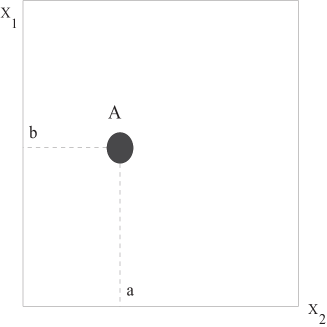
Figure 1: Geometrical interpretation of fuzzy sets. The fuzzy subset A is a point in the unit 2-cube with coordinates a and b. The cube consists of all possible fuzzy subsets of two elements, @$x_{i}$ and $x_{j}$.

membership $(\Psi\Psi^{*})_{i}\Delta V_{i}$ at each vertex of the infinite-dimensional hypercube and multiply it by the value of the physical quantity at the respective point $x_{i}$. Summing over all these products results in the averaged (defuzzified) value of the quantity.

Thus, instead of averaging over the distribution of random quantities, we introduce the defuzzification of deterministic quantities. Mathematically both processes are identical, but physically they are absolutely different. We do not need any more the probabilistic interpretation of the wave function $\Psi$, which implies that there is another, more detailed level of description that would allow us to get rid of uncertainties introduced by randomness. Now it is clear that, within the framework of the fuzzy interpretation, we cannot get rid of the uncertainties intrinsic to fuzziness (and not connected to randomness). From this point of view quantum mechanics does not need any hidden variable to improve its predictions. They are precise within the framework of the fuzzy theory.

Moreover, since quantum mechanics is a linear theory, one can speculate that according to the fuzzy approximation theorem [13] the linearity and fuzziness of quantum mechanics are the best tools to approximate (with any degree of accuracy) any macrosystem (linear or nonlinear). The linearity of quantum mechanics is responsible for the uncertainty relations which are present in any linear system. Therefore (as was demonstrated long time ago [5]), these relations enter quantum mechanics even before any concept of measurement.

Let us consider the membership density of a free microobject (a progenitor of a classical free particle). It is obvious that $\Psi\Psi^{*}=const$. This means that the relative degree of membership for any two points in space is 1. In other words, the free microobject is ”everywhere,” the same property that is characteristic for a three-dimensional standing wave. In particular, this example shows that the wave-particle duality is not necessarily a duality but rather an expression of the fuzzy nature of things quantum.

In fact, we can even go that far as to claim that the complementarity principle is a product of a compromise between the requirements of the bivalent logic and the results of quantum experiments. Within the framework of the fuzzy approach there is no need to require complementarity, since the logic of a fuzzy microobject transcends the description of its properties in terms of either/or and, as a result, is much more complete, probably the most complete description under the given experimental results.

It turns out that the membership density has something more to offer than simply a degree to which a fuzzy microobject has a membership in a certain elemental volume dV. In fact, using the expansion of the wave amplitude (we could call it ”fuzziness amplitude”) in its orthonormal eigenfunctions $\Psi$ and assuming that the integral in (20) is bounded, we write the well-known expression

$$\int_{-\infty}^{\infty}\Psi\Psi^{*}dV=\sum_{k=1}^{\infty}a_{k}a_{k}^{*}=1$$ (21)

Equation (21) allows a very simple geometric interpretation with the help of a $(N-1)$-dimensional simplex. A fuzzy state $\Psi$ is represented as a point $A$ at the boundary of this simplex. (Figure 2 shows this for a one-dimensional simplex, $k=1,2.$) Its projections onto the respective axes correspond to the values $a_{k}a_{k}^{*}$.

Now applying the subsethood theorem [6], we interpret the values of $a_{k}a_{k}^{*}$ as the degree to which the state A is contained in a particular eigenstate $k$. Using Fig. 2 we can clearly see that $A\cap B=B,A\cap C=C$. Moreover, the same figure shows that the lengths of projections of A onto the respective axes (namely, OA and OC) are nothing but the cardinality sizes $M(A\cap B)=a_{1}a_{1}^{*}$ and $M(A\cap C)=a_{2}a_{2}^{*}$. On the other hand, the cardinality size of A is $M(A)=1$. Therefore, the respective subsethood measures are $S(A,B)=a_{1}a_{1}^{*}/1$ and $S(A,C)=a_{2}a_{2}^{*}/1.$ At the same time, both of these measures provide a number of detections (successful outcomes) of the respective states $k=1$ or $k=2$ in the repeated experiments.

Our discussions is applicable to a particular case of a state A described by a wave (fuzziness) amplitude $\Psi$ corresponding to a pure state. However it is general enough to describe a mixed state characterized by the density matrix $\rho(x^{\prime},x)$. The integral of $\rho(x^{\prime},x)$ over all $x^{\prime}s$ yields the sum $\sum_{k=1}^{\infty}a_{kk^{\prime}}$ which is the generalization of a measure of containment of the fuzzy state A in the discrete states k.

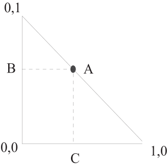
Figure 2: Representation of a quantum mechanical state $A$ as a point in a one-dimensional fuzzy simplex

By preparing a certain state, which is now understood to be a fuzzy entity, we fix the frequencies of the experimental realizations of this fuzzy state in its substates $k$. If the fuzzy state A undergoes a continuous change, which corresponds in Fig. 2 to motion of point A along the hypotenuse, then its subsethood in any state $k$ changes. This implies the following: if the eigenfunctions of a fuzzy set stay the same, the degree to which the respective eigenstates represent the fuzzy state varies. The variation can occur continuously despite the fact that the eigenstates are discrete.

This indicates an interesting possibility that quantum mechanics is not necessarily tied to the Hilbert space. Such a possibility was mentioned long ago by von Neumann [14] and recently was addressed by Wulfman [15]. One of the hypothetical applications of this idea is to use quantum systems as an infinite continuum state machine in a fashion that is typical for a fuzzy system: small continuous changes in the input from some ”ugly” nonlinear system will result in small changes at the output of the quantum system which in turn can be correlated with the input to produce the desired result.

Concluding our introduction to a connection between fuzziness and quantum mechanics, we prove a statement that can be viewed as a generalized Ehrenfest theorem. We will demonstrate that defuzzification of the Schroedinger equation (with the help of the membership density $\Psi\Psi^{*}$) yields the Hamilton-Jacobi equation. This will provide $\it{aposteriori}$ derivation of the Schroedinger equation for an arbitrary potential $V({\bf{x}},t)$. We assume that the fuzzy amplitude $\Psi\rightarrow 0$ as ${\bf{x}}\rightarrow\infty$ and rewrite the Schroedinger equation as follows:

$$\frac{\hbar}{i}\frac{\partial ln\Psi}{\partial t}+\frac{\hbar^{2}}{2m}{(\nabla ln\Psi)}^{2}+V=0$$ (22)

Integrating (22) with the weight $\Psi\Psi^{*}$ (i.e., ”defuzzifying” it), we obtain

$$\int\Psi\Psi^{*}[\frac{\hbar}{i}\frac{\partial ln\Psi}{\partial t}+\frac{\hbar^{2}}{2m}{(\nabla ln\Psi)}^{2}+V]d^{3}x=0$$ (23)

Integrating the second term by parts and taking into account that the resulting surface integral vanishes because $\Psi\rightarrow 0$ at infinity, we obtain the following equation:

$$\langle\frac{\partial S}{\partial t}\rangle+\frac{1}{2m}\langle\nabla S\nabla S^{*}\rangle+\langle V\rangle=0$$ (24)

where $\langle\rangle$ denote defuzzification with the weight $\Psi\Psi^{*}$, and $S=(\hbar/i)ln\Psi$. This equation is analogous to the classical Hamilton-Jacobi equation (4).

The generalized Ehrenfest theorem shows that the classical description is true only on a coarse scale generated by the process of ”defuzzification,” or measurement. The ”classical measurement” corresponds to the introduction of a non-quantum concept of the potential $V({\bf{x}},t)$ serving as a shorthand for the description of a process of interaction of a microobject (truly quantum object) with a multitude of other microobjects. This process destroys a pure fuzzy state (a constant fuzziness density) of a free quantum ”particle.”

Paraphrasing Peres, [16] we can say that a classical description is the result of our ”sloppiness,” which destroys the fuzzy character of the underlying quantum mechanical phenomena. This means that, in contradistinction to Peres, we consider these phenomena ”fuzzy” in a sense that the respective membership distribution in quantum mechanics does not have a very sharp peak, characteristic of a classical mechanical phenomena. Note that we exclude from our consideration the problem of the classical chaos,assuming that our repeated experiments are carried out under the absolutely identical conditions.

5 CONCLUSION

This work represents a continuation of our previous effort [1] to understand quantum mechanics in terms of the fuzzy logic paradigm. We regard reality as intrinsically fuzzy. In spatial terms this is often called nonlocality. Reality is nonlocal temporarily as well, which means that any microobject has membership (albeit to a different degree) in both the future and the past. In this sense one might define the present as the time average over the membership density. A measurement is defined as a continuous process of defuzzification whose final stage, detection, is inevitably accompanied by a dramatic loss of information through the emergence of locality, or crispness, in fuzzy logic terms.

We have attempted to provide a description of quantum mechanics in terms of a deterministic fuzziness. It is understood that this attempt is inevitably incomplete and has many features that can be improved, extended, or corrected. However, we hope that this work will inspire others to start looking at the quantum phenomena through ”fuzzy” eyes, and perhaps something practical (apart from removing wave-particle duality and complementarity mysteries) will come out of this.

Acknowledgment

One of the authors (AG) wishes to thank V. Panico for very long and very illuminating discussions, which helped to shape this work, and for reading the manuscript. HJC’s work was supported by the Air Force Office of Scientific Research

References

- [1] H. Caulfield and A. Granik, Spec. Sci. Tech. 18, 61 (1995).
- [2] B. Kosko, Fuzzy Thinking (Hyperion, NY, 1993), p. 18.
- [3] I. Percival, in Quantum Chaos-Quantum Measurement, edited by P. Cvitanovic, I. Percival, and A. Wirzbe (Kluwer Academic, Dordrecht, 1992), p. 199.
- [4] M. Krieger, Doing Physics (Indiana University Press, 1992), p. XX.
- [5] L. Mandel’shtam, Lectures on Optics, Relativity, and Quantum Mechanics (Nauka, Moscow, 1972), p. 332.
- [6] B. Kosko, Neural Networks and Fuzzy Systems (Prentice-Hall, Englewood Cliffs, NJ, 1992), Chap. 1.
- [7] L. Zadeh, Informal. Control 8, 338 (1965).
- [8] P. Dirac, The Principles of Quantum Mechanics (Oxford, 1957), p. 10.
- [9] B. Kosko, Int. J. Gen. Syst. 17, 211 (1990).
- [10] E. Schroedinger, Collected Papers on Quantum Mechanics (Chelsea, NY, 1978), p. 26.
- [11] D. Bohm, in Problems of Causality in Quantum Mechanics (Nauka, Moscow, 1955), p. 34.
- [12] R. Feynman and A. Hibbs, Quantum Mechanics and Path Integrals (McGraw-Hill, NY, 1965), Chap. 3.
- [13] B. Kosko, in Proceedings of the First I.E.E.E. Conference of Fuzzy Systems (IEEE Proceedings, San Diego, 1992), p. 1153.
- [14] G. Birkgoff and J. von Neumann, Ann. Math. 37, 823 (1936).
- [15] C. Wulfman, Int. J. Quantum Chem. 49, 185 (1994).
- [16] A. Peres, in Ref. 4, p. 249.