Quantum-scissors device for optical state truncation:
A proposal for practical realization

Abstract

We propose a realizable experimental scheme to prepare superposition of the vacuum and one-photon states by truncating an input coherent state. The scheme is based on the quantum scissors device proposed by Pegg, Phillips, and Barnett [Phys. Rev. Lett. 81, 1604 (1998)] and uses photon-counting detectors, a single-photon source, and linear optical elements. Realistic features of the photon counting and single-photon generation are taken into account and possible error sources are discussed together with their effect on the fidelity and efficiency of the truncation process. Wigner function and phase distribution of the generated states are given and discussed for the evaluation of the proposed scheme.

DOI: 10.1103/PhysRevA.64.0638XX         PACS number(s): 42.50.Dv, 42.50.Ar, 03.65.Ta, 03.67.-a

]

I Introduction

There has been a growing interest in the generation and engineering of quantum states of light. Over the last decade, various schemes for preparation of Fock states [2] and their arbitrary finite superpositions [3, 4, 5, 6, 7, 8, 9, 10, 11] have been developed. The motivation behind these efforts is the possible applications of nonclassical states of light in quantum communication and information processing. Such states have been shown to be generated by nonlinear media or by conditional measurements at the output ports of beam splitters. For example, the method proposed by Dakna et al. [6] relies on an alternate application of coherent displacement and photon adding (and/or subtracting) via conditional measurements on beam splitters for the generation of several different types of nonclassical states. That scheme consists of photon-counting devices, high-transmittance beam splitters, and the condition of no-photon detection at the detectors. Another interesting scheme proposed by D’Ariano et al. [7] is based on ring cavity and Kerr medium. However, the simplest scheme is the one proposed by Pegg and co-workers [4, 5]. This scheme (see Fig. 1), referred to as the quantum scissors device (QSD), enables generation of the finite superpositions of number states by truncating a coherent state. Recently, Resch et al. proposed and experimentally demonstrated a QSD-like state-preparation technique based on conditional coherence [8].

The quantum scissors device exploits three fundamental concepts of quantum mechanics: (a) Entanglement, mixing of vacuum and a single photon at the first beam splitter (BS1) creates an entangled state and opens a quantum channel; (b) measurement, a physical system can be brought to a desired state by a conditional measurement; and (c) nonlocality, vacuum and single-photon components of the coherent state at ${\hat{b}}_{3}$ are generated at the ${\hat{b}}_{1}$ mode without any light going from ${\hat{b}}_{3}$ of the second beam splitter (BS2) to ${\hat{b}}_{1}$ mode of BS1. Recently, the basic idea of the QSD has been slightly modified to generate the superposition of vacuum, one-photon, and two-photon states [9]. An interferometric scheme equivalent to a QSD with tunable beam splitters has been proposed by Paris to prepare arbitrary superposition states [12]. It has also been shown that the basic QSD scheme can be applied as a teleportation device for superposition states [13]. No proposal has been made concerning the practical scheme of the QSD, which considers realistic models for the detectors and sources.

In this paper, our main interest is to propose and study an experimental QSD scheme for producing superposition of the vacuum and one-photon states, $C_{0}|0\rangle+C_{1}|1\rangle$, which is the simplest optical-qubit state with phase information. The paper is organized as follows. In Sec. II, a schematic configuration of the Pegg-Phillips-Barnett

FIG. 1.: Schematic configuration of the quantum scissors device (QSD). BS1, BS2, beam splitters; $D_{2}$, $D_{3}$, photon counting detectors; $|\alpha\rangle$, $|0\rangle$, $|1\rangle$, coherent, vacuum, and single-photon states, respectively; $|\Phi_{\rm trunc}\rangle$, truncated output state.

QSD scheme is given and theoretical background is discussed. We will consider an ideal scheme to study the effects of beam splitter parameters on the fidelity of the output state and the efficiency of truncation process. In Secs. III and IV, the proposed experimental setup is introduced, the possible sources of error (imperfections in detectors and single-photon source) and their effects on the preparation of the desired state are studied. To evaluate the feasibility of the scheme, the fidelity of the output state and the rate of preparing it are discussed. Section V includes a comparison of fidelities for different states. In Sec. VI, the Wigner function and its marginals for the generated states are analyzed. Finally, a discussion of the results is given in Sec. VII.

II Quantum scissors device: Schematics and principles

The basic scheme of the QSD proposed by Pegg et al. is shown in Fig. 1. It consists of two beam splitters and two photon counters. The input modes of the setup are denoted as ${\hat{a}}_{1}$, ${\hat{a}}_{2}$, and ${\hat{b}}_{3}$. The actions of beam splitters can be described as unitary transformations of the operators in the Heisenberg picture, which can be written as [14]

$$\hat{R}_{1}\hat{a}_{1}^{\dagger}\hat{R}_{1}^{\dagger} =t_{1}\hat{b}_{1}^{\dagger}-r_{1}^{*}\hat{b}_{2}^{\dagger}~{},\quad\hat{R}_{1}\hat{a}_{2}^{\dagger}\hat{R}_{1}^{\dagger} =r_{1}\hat{b}_{1}^{\dagger}+t_{1}^{*}\hat{b}_{2}^{\dagger},$$ (1)

$$\hat{R}_{2}\hat{b}_{3}^{\dagger}\hat{R}_{2}^{\dagger} =t_{2}\hat{c}_{3}^{\dagger}-r_{2}^{*}\hat{c}_{2}^{\dagger}~{},\quad\hat{R}_{2}\hat{b}_{2}^{\dagger}\hat{R}_{2}^{\dagger} =r_{2}\hat{c}_{3}^{\dagger}+t_{2}^{*}\hat{c}_{2}^{\dagger},$$ (2)

where $\hat{R}_{1}$ and $\hat{R}_{2}$ are the unitary operators satisfying $\hat{R}_{1}|00\rangle_{(a_{1},a_{2})}=|00\rangle_{(b_{1},b_{2})}$ and $\hat{R}_{2}|00\rangle_{(b_{2},b_{3})}=|00\rangle_{(c_{2},c_{3})}$. $t_{j}$ and $r_{j}$ are the beam-splitter complex transmission and reflection coefficients satisfying $|t_{j}|^{2}+|r_{j}|^{2}=1$, and $(^{*})$ denotes complex conjugation.

In the QSD scheme, BS1 is fed by a single photon in mode ${\hat{a}}_{1}$ and mode ${\hat{a}}_{2}$ is left in vacuum. Using the relations given in Eq. (2), the output of the beam splitter is found to be an entangled state that can be written as

$$|\psi\rangle_{(b_{1},b_{2})}=\hat{R}_{1}|10\rangle_{(a_{1},a_{2})}=t_{1}|1\rangle_{b_{1}}|0\rangle_{b_{2}}-r^{*}_{1}|0\rangle_{b_{1}}|1\rangle_{b_{2}}.$$ (3)

The output mode ${\hat{b}}_{2}$ is then fed into BS2 where it is mixed with mode ${\hat{b}}_{3}$ prepared in a coherent state

$$|\alpha\rangle_{b_{3}}=e^{-|\alpha|^{2}/2}\sum_{n=0}^{\infty}\frac{\alpha^{n}}{n!}(\hat{b}_{3}^{\dagger})^{n}|0\rangle_{b_{3}},$$ (4)

which will be truncated to prepare the desired superposition of vacuum and one-photon states

$$|\varphi_{\rm desired}\rangle_{b_{1}}=\frac{1}{\sqrt{1+|\alpha|^{2}}}(|0\rangle_{b_{1}}+\alpha|1\rangle_{b_{1}}).$$ (5)

As a result of the action of BS2 with $t_{2}$ and $r_{2}$, the state at three modes becomes

$$|\Psi\rangle_{(b_{1},c_{2},c_{3})}=e^{-|\alpha|^{2}/2}\sum_{n=0}^{\infty}\sum_{k=0}^{n}\frac{\alpha^{n}(-r^{*}_{2})^{k}(t_{2})^{n-k}}{\sqrt{k!(n-k)!}}$$ (6)

$$\quad\times(t_{1}|1,k,n-k\rangle-\sqrt{(n-k+1)}r^{*}_{1}r_{2}|0,k,n-k+1\rangle$$ (7)

$$\quad-\sqrt{(k+1)}r^{*}_{1}t^{*}_{2}|0,k+1,n-k\rangle).$$ (8)

Both output modes of BS2 are measured with photon-counting detectors. The output state generated at mode ${\hat{b}}_{1}$ of BS1 depends on the outcome of the measurements at the detectors. A normalized superposition of zero- and one-photon states

$$| \Phi_{\rm trunc}\rangle_{b_{1}}={\cal N}\,_{(c_{2},c_{3})}\langle 1,0|\Psi\rangle_{(b_{1},c_{2},c_{3})}$$ (10)

$$\;\;\;=\frac{1}{\sqrt{|r_{1}t_{2}|^{2}+|\alpha|^{2}|r_{2}t_{1}|^{2}}}[(r_{1}t_{2})^{*}|0\rangle_{b_{1}}+r^{*}_{2}t_{1}\alpha|1\rangle_{b_{1}}],$$

where ${\cal N}$ is the renormalization constant, can be obtained at the output of the QSD upon detection of one photon at $D_{2}$ and no photon at $D_{3}$.

Although this scheme can also be used to obtain any desired superposition of vacuum and single-photon states by proper choice of beam-splitter parameters and $\alpha$, we will consider only the truncation process in this study. The fidelity of the output truncated state to any desired state can be calculated from

$$F=~{}_{b_{1}}\langle\varphi_{\rm desired}|\hat{\rho}_{\rm trunc}|\varphi_{\rm desired}\rangle_{b_{1}}$$ (11)

with $\hat{\rho}_{\rm trunc}=|\Phi_{\rm trunc}\rangle_{b_{1}b_{1}}\langle\Phi_{\rm trunc}|$. Then the fidelity of preparing the truncated coherent state up to single-photon state can be found as

$$F=\frac{|r_{1}t_{2}|^{2}+|\alpha|^{2}(r_{1}^{*}r_{2}t_{1}^{*}t_{2}^{*}+r_{1}r_{2}^{*}t_{1}t_{2})+|\alpha|^{4}|t_{1}r_{2}|^{2}}{(|r_{1}t_{2}|^{2}+|\alpha|^{2}|t_{1}r_{2}|^{2})(1+|\alpha|^{2})},$$ (12)

which shows that the fidelity of the truncation process depends on the beam splitter-parameters and the intensity of the input coherent light. Without loss of generality, we can take $r_{1}={\rm i}|r_{1}|$, $r_{2}={\rm i}|r_{2}|$, $t_{1}=|t_{1}|$, and $t_{2}=|t_{2}|$ for which

$$|\Phi_{\rm trunc}\rangle_{b_{1}}=\frac{|r_{1}t_{2}||0\rangle_{b{1}}+\alpha|r_{2}t_{1}||1\rangle_{b{1}}}{\sqrt{|r_{1}t_{2}|^{2}+|\alpha|^{2}|r_{2}t_{1}|^{2}}}$$ (13)

is obtained. In that case, the dependence of truncation fidelity on beam-splitter parameters for an input coherent light of $|\alpha|^{2}=1$ will be as shown in Fig. 2(a). It can be seen from this figure that perfect fidelity $(F=1)$ is achieved for a range of beam-splitter parameters satisfying $|t_{1}|^{2}-|t_{2}|^{2}=0$. However, the efficiency of truncation, which can be defined as the probability of the desired detection, is different for different choices of beam-splitter parameters and can be calculated as

$$P_{\rm detection} = |\,_{(c_{2},c_{3})}\langle 1,0|\Psi\rangle_{(b_{1},c_{2},c_{3})}|^{2}$$ (14)

$$= (|r_{1}t_{2}|^{2}+|\alpha|^{2}|t_{1}r_{2}|^{2})e^{-|\alpha|^{2}}\equiv{\cal N}^{-2}.$$ (15)

(a)                                   (b)

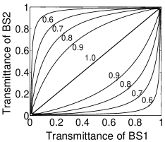
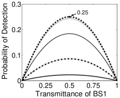
FIG. 2.: Effect of beam-splitter parameters (transmittances $|t_{1}|^{2}$ and $|t_{2}|^{2}$) and intensity of the input coherent light on (a) the fidelity and (b) efficiency of truncation process (probability of proper detection). Curves (a) are plotted for constant fidelity. In (b), beam splitters are considered to be the same (thus $F=1$) and curves from top to bottom correspond to $|\alpha|^{2}=0.1,~{}0.5,~{}1.0,~{}1.5,$ and $2.0$, respectively. The highest probability of detection is $\sim 0.25$.

$P_{\rm detection}$ is depicted in Fig. 2(b) from which it can be concluded that the highest $P_{\rm detection}$ for $F=1$ is achieved when two identical 50:50 beam splitters are used. A fidelity of $F=1$ is achieved with $\max(P_{\rm detection})=0.184$ when $|\alpha|^{2}=1$ and $|t_{1}|^{2}=|t_{2}|^{2}=0.5$.

Further analysis of Eq. (8) shows that detection of one photon at $D_{3}$ and no photon at $D_{2}$ will yield the following truncated state:

$$|\Phi_{\rm trunc}^{{}^{\prime}} \rangle_{b_{1}}={\cal N}\,^{\prime}\,_{(c_{2},c_{3})}\langle 0,1|\Psi\rangle_{(b_{1},c_{2},c_{3})}$$ (16)

$$= \frac{1}{\sqrt{|r_{1}r_{2}|^{2}+|\alpha|^{2}|t_{1}t_{2}|^{2}}}(r^{*}_{1}r_{2}|0\rangle_{b_{1}}-t_{1}t_{2}\alpha|1\rangle_{b_{1}}),$$ (17)

where ${\cal N}\,^{\prime}$ is the renormalization constant. Substituting imaginary reflection and real transmission coefficients as above will give a superposition state for which the relative phase between $|0\rangle_{b_{1}}$ and $|1\rangle_{b_{1}}$ components is $\pi$ shifted from that of Eq. (13). This phase shift can be corrected by a unitary transformation of Pauli operator $\sigma_{z}$ after the detection. Then the use of beam splitters with parameters satisfying $|t_{1}|^{2}+|t_{2}|^{2}=1$ will give an output state with $F=1$. For this detection case, too, the highest probability of generating an output state with perfect fidelity is obtained for beam splitters with $|t_{1}|^{2}=|t_{2}|^{2}=0.5$. In fact, under these conditions, if $\sigma_{z}$ rotation is allowed, a successful truncation is possible when the number of photons detected at $D_{2}$ and $D_{3}$ differs by unity [5].

III Experimental scheme for a realistic QSD

We propose the scheme of the realistic QSD, given in Fig. 3, that can be implemented in practice. One part of this scheme uses the ideas developed and illustrated by Rarity and co-workers [15]. The output light of a pulsed laser with angular frequency $\omega_{0}$ is divided into two by a beam splitter. Transmitted part of the light is frequency doubled in a nonlinear crystal and the resultant pulses of frequency $2\omega_{0}$ are used to pump a nonlinear crystal to induce spontaneous parametric down-conversion (SPDC). The crystal is for type-I degenerate phase matching, which produces down-converted photon pairs in two modes (idler and signal) with the same polarization and at roughly half the frequency of the pumping pulses on opposite sides of a cone whose opening angle depends on the angle between the optical axis of the crystal and the pump. The pump field at the output of the crystal is eliminated by a beam-stopping mirror. The signal and idler photons are selected by the apertures and directed to narrow-band filters where the background radiation is eliminated and the selection is further restricted to only the degenerate photons. The selected idler mode ${\hat{c}}_{1}$ is directed to the first photon-counting detector $D_{1}$, which is considered as a gating detector, where a “click” upon the detection of a photon in idler mode ensures the presence of another photon in the signal mode ${\hat{a}}_{1}$. The latter is input to the (50:50) BS1 at mode ${\hat{a}}_{1}$ and mixed with vacuum at mode ${\hat{a}}_{2}$ resulting in an entangled state at the output of BS1. The undoubled laser light beam (reflected portion at BS) is attenuated and directed to the input mode ${\hat{b}}_{3}$ of the (50:50) BS2. Then it is mixed with the entangled state at the output mode of BS1, which is fed into the other input mode of BS2. Temporal overlapping of these two inputs at BS2 can be satisfied by adjusting the variable delay placed in the path of the weak coherent state. The resultant states at the output modes of BS2 are passed through apertures and narrow-band filters before reaching the photon-counting detectors. Detection of a photon at $D_{2}$ of mode ${\hat{c}}_{2}$ and no photons at $D_{3}$

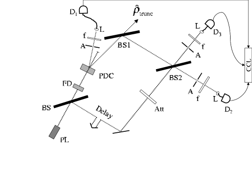
FIG. 3.: Proposed experimental scheme for the QSD. PL, pulsed laser; FD, frequency doubler; PDC, parametric down conversion crystal; Att, strong attenuator; A, aperture; f, narrow band filter; L, lens; CCL, coincidence counter and logic; BS, BS1, and BS2 are beam splitters; and $D_{1}$, $D_{2}$, and $D_{3}$ are photon-counting detectors.

of mode ${\hat{c}}_{3}$ will ensure the preparation of the desired truncated state at the output mode ${\hat{b}}_{1}$ of BS1. The filters and apertures in the scheme are used to make the weak coherent light indistinguishable from the entangled state entering into the other input mode of BS2. In the scheme, the output state is conditioned on coincidence detection at $D_{1}$ and $D_{2}$, and anticoincidence at $D_{3}$.

Now, let us analyze the outlined system considering only the effects of beam splitters and detectors. Using Eq. (2), the output of a beam splitter can be calculated by $\hat{R}\hat{\rho}_{{\rm in}}\hat{R}^{\dagger}$ for a given input density operator $\hat{\rho}_{\rm in}$. If the output signal of the SPDC is $\hat{\rho}_{(a_{1},c_{1})}$ then the input state-density operator of the BS1 will be $\hat{\rho}_{{\rm in}1}=\hat{\rho}_{(a_{1},c_{1})}\otimes|0\rangle_{a_{2}{a_{2}}}\langle 0|$. With this input, output of BS1 will be $\hat{\rho}_{(b_{1},b_{2},c_{1})}=\hat{R}_{1}\hat{\rho}_{{\rm in}1}\hat{R}_{1}^{\dagger}$. Considering that the state at ${\hat{b}}_{3}$ mode of BS2 is coherent $|\alpha\rangle_{b_{3}b_{3}}\langle\alpha|$, input density operator of BS2 becomes $\hat{\rho}_{{\rm in}2}=\hat{\rho}_{(b_{1},b_{2},c_{1})}\otimes|\alpha\rangle_{b_{3}{b_{3}}}\langle\alpha|$, then letting this operator evolve through the BS with $\hat{R}_{2}$, we obtain the following output density operator

$$\hat{\rho}_{{\rm out}} = \hat{\rho}_{(b_{1},c_{1},c_{2},c_{3})}=\hat{R}_{2}\hat{\rho}_{{\rm in}2}\hat{R}_{2}^{\dagger}$$ (18)

$$= \hat{R}_{2}(\hat{\rho}_{(b_{1},b_{2},c_{1})}\otimes|\alpha\rangle_{b_{3}}\,{}_{b_{3}}\!\langle\alpha|)\hat{R}_{2}^{\dagger}$$ (19)

$$= \hat{R}_{2}\hat{R}_{1}(\hat{\rho}_{(a_{1},c_{1})}\otimes|0\rangle_{a_{2}}\,{}_{a_{2}}\!\langle 0|\otimes|\alpha\rangle_{b_{3}}\,{}_{b_{3}}\!\langle\alpha|)\hat{R}_{1}^{\dagger}\hat{R}_{2}^{\dagger}.$$ (20)

The normalized truncated output state density operator at mode ${\hat{b}}_{1}$ of BS1 is obtained by

$$\hat{\rho}_{\rm trunc}=\frac{{\rm{Tr}}_{(c_{1},c_{2},c_{3})}(\Pi_{1}^{c_{1}}\Pi_{1}^{c_{2}}\Pi_{0}^{c_{3}}\hat{\rho}_{{\rm out}})}{{\rm{Tr}}_{(b_{1},c_{1},c_{2},c_{3})}(\Pi_{1}^{c_{1}}\Pi_{1}^{c_{2}}\Pi_{0}^{c_{3}}\hat{\rho}_{{\rm out}})}\,,$$ (21)

where $\Pi_{1}^{c_{1}}$, $\Pi_{1}^{c_{2}}$, and $\Pi_{0}^{c_{3}}$ are elements of the positive-operator-valued measures (POVM’s) for the detectors $D_{1}$, $D_{2}$, and $D_{3}$, respectively, with zero and one corresponding to the number of clicks recorded at the detectors.

IV Error sources in QSD scheme

In the following, we assume that the apertures, narrow-band filters, and delays introduced in the scheme ensure the proper phase and mode matching at the beam splitters. Thus, we will study only the imperfections in the single-photon generation and photon-counting devices, and their effects on the feasibility of the QSD scheme.

A Nonideal single-photon source

In the proposed scheme SPDC is used as the source for the preparation of the single-photon state at the input of the BS1. In practice, we must take into account some basic features of SPDC as a source. First, although the conservation of energy forces the sum of the frequencies of the idler and signal photons to be equal to the frequency of the pump field, the photons may have finite bandwidth due to the finite size of the crystal. Second is the spatial location of the idler and signal photons in the cone of radiation at the crystal output. These two problems can be solved approximately by spatial and frequency filtering as explained above. The third one is the intrinsic property of SPDC, that is, the output of SPDC contains vacuum with high probability while the probability of a photon-pair generation is very low. Even though the probability is much lower, there may be cases where more than one photon pair is generated. In SPDC, photons are generated in pairs with equal numbers in the signal ($\hat{a}_{1}$) and idler ($\hat{c}_{1}$) modes as can be seen in the expression for the state at the output of the SPDC crystal [16],

$$|\varphi\rangle_{(a_{1},c_{1})}=\sqrt{1-\gamma^{2}}\sum_{k=0}^{\infty}(\gamma e^{{\rm i}\theta_{\rm p}})^{k}|k\rangle_{a_{1}}|k\rangle_{c_{1}}\,,$$ (22)

where $\gamma=\tanh(|\kappa\tau|)$ and $\gamma^{2}$, typically $\sim 10^{-4}$/pulse [17], corresponds to the rate of one-photon-pair generation per pulse of the pump field; $\kappa$ represents the product of coupling constant and the complex amplitude of the pump field; and $\tau$ stands for the interaction time of the pump field and the crystal. The phase of the pump field is denoted by $\theta_{\rm p}$. In the proposed experimental scheme, we suppose that the explicit information of the phase $\theta_{\rm p}$ is not known, which results in the following mixed state for the output of SPDC after averaging over all possible phases:

$$\hat{\rho}_{(a_{1},c_{1})} = (1-\gamma^{2})[|00\rangle\langle 00|+\gamma^{2}|11\rangle\langle 11|$$ (24)

$$+\gamma^{4}|22\rangle\langle 22|+\gamma^{6}|33\rangle\langle 33|+\cdots]_{(a_{1},c_{1})}$$

In the following, Eq. (24) will be used for numerical simulations.

B Imperfect photon counting detectors

Photodetection is the very basis of quantum-optical measurements. Currently most commonly used photodetectors are avalanche photodiodes that suffer from four main problems (a) nonunit efficiency $(\eta\neq 1)$ causing the failure of photon detection, (b) nonzero dark count $\nu\neq 0$ causing “false alarms” by signal generation even when there is no photon, (c) failure to discriminate between $n$ and $n+1$ photons if $n\geq 1$, and (d) “dead time” $\tau_{\rm dt}$ of the photon-counting detector and the processing electronics during which detectors cannot respond to the incoming photons.

After the arrival of the first photon to a detector, a time duration of $\tau_{\rm dt}$ should pass for the detector to count the next coming photons. If the arrival times of photons at the detector are less than $\tau_{\rm dt}$, then only one electronic

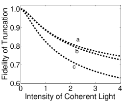
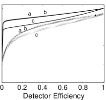
FIG. 4.: Effect of intensity of coherent light, $|\alpha|^{2}$, (left) and the detector efficiency $\eta$ (right) on the fidelity $F$ of truncation process for photon-number-discriminating counters and $\gamma^{2}=5\times 10^{-4}$/pulse. $a$, $b$, and $c$ correspond to $(1,0)$, $(2,1)$, and $(3,2)$, respectively, which stand for the number of photons detected at the detectors ($D_{2}$,$D_{3}$). Left plot was obtained for $R_{\rm dark}=1000~{}{\rm s}^{-1}$ and $\eta=0.5$. Right plot is for $|\alpha|^{2}=0.4$ with solid and dotted curves corresponding to $R_{\rm dark}=100~{}{\rm s}^{-1}$ and $R_{\rm dark}=10^{4}~{}{\rm s}^{-1}$, respectively.

pulse, which corresponds to the detection of the first photon, will be generated. The average counting rate should be less than $1/\tau_{\rm dt}$ to eliminate the effect of dead time on the counted photon rate. In the QSD scheme, “dead time” shows itself in two ways. (i) For $D_{1}$ and $D_{2}$ detectors, if a photon is incident on the detector within $\tau_{\rm dt}$ seconds after the preceding photon, then the event will just be neglected and we will not count the output state as the desired one. The effect of such a case will be the reduction in the number of states generated per second. (ii) There may be cases where $D_{1}$ and $D_{2}$ detect photons and even though there is an incident photon on $D_{3}$, it does not click because it is still “dead.” Such a case will be counted as the desired detection and a state different from the desired one will be prepared at the output, which will decrease the fidelity of the prepared states. Both of these two cases can be considered as the loss of photon due to inefficient detection. A decision on the outcome of the measurement is done for each light pulse separately, independent of the result of the preceding or the following pulses. Moreover, we are not interested in the correlation between two consecutive pulses. Therefore, the effect of dead time can be absorbed into the detector efficiency $\eta$. Typical values for dead time have been reported to be in the range 30 ns $\leq\tau_{\rm dt}\leq$ 100 ns for million counts per second [18]. In order to minimize the effect of dead time, one has either to use very weak light so that the number of photons in the system per second is low enough, or to work with small repetition frequency for the input coherent light and the pump of the SPDC crystal.

For a realistic description of photon-counting detectors ($D_{1}$, $D_{2}$, and $D_{3}$) shown in Fig. 3, POVM can be written as [19]

$$\Pi_{N}=\sum_{n=0}^{N}\sum_{m=n}^{\infty}\frac{e^{-\nu}\nu^{N-n}}{(N-n)!}\eta^{n}(1-\eta)^{m-n}C^{m}_{n}|m\rangle\langle m|$$ (25)

for a detector with quantum efficiency $\eta$ (dead-time effects are included) and mean dark count of $\nu$, where $\sum_{N=0}^{\infty}\Pi_{N}=1$. In this equation $n$ is the actual number of photons present in the mode, $N-n$ is the number of dark counts, $N$ is the number of “clicks,” and $C^{m}_{n}$ is the binomial coefficient. Mean dark count rate is given by $\nu=\tau_{\rm res}R_{\rm dark}$, where $R_{\rm dark}$ is the dark count rate and $\tau_{\rm res}$ is the resolution time of the detector and the electronic circuitry and is longer than the pulse width $\tau_{p}$ of the pulsed light used in the experiment. In the following, we will work with three kinds of detectors (photon-number-discriminating detector, conventional photon counter, and single-photon counter) in order to show the effects of imperfections (a)-(c) and detector types on the properties of truncated states using POVM for each type of detector. We will assume a pump with a repetition frequency of 100 MHz and the detector resolution time $\tau_{\rm res}$=10 ns.

1 Photon-number-discriminating counter (PNDC)

Although not available in the market, the analysis of the system with PNDC will give us a reference for comparison with other detector types. The POVM for this kind of detectors is given by Eq. (25). For this type of detectors, if the ideal case (unit efficiency, no dark count, and perfect single-photon source) is considered, the same result shown in Eq. (5) is obtained. In Fig. 4, we show the dependence of fidelity of truncation with the experimental scheme if all three detectors are PNDC. In this figure, we see that increasing coherent light intensities $|\alpha|^{2}$ causes a decrease in the fidelity of truncation for all detection cases. In the cases where $(1,0)$ and $(2,1)$ photons are detected at detectors ($D_{2}$,$D_{3}$), fidelity of truncation is almost the same, however, for other cases $(n>2,~{}m>1)$, $F$ decreases sharply with increasing light intensities and dark count rates. We have also observed that for increasing light intensities, the effect of $\eta$ become very deleterious (not shown in Fig. 4). However, for $|\alpha|^{2}\ll 1$, it does not constitute a major problem and the fidelity of truncation is essentially insensitive to changes in $\eta$.

2 Conventional photon counter (CPC)

This type of detectors can only distinguish between the presence and absence of photons in the mode by a “click” or “no click.” No information on the exact number of photons can be obtained in a single click. Then the POVM can be written as

$$\Pi_{0} = \sum_{m=0}^{\infty}e^{-\nu}(1-\eta)^{m}|m\rangle\langle m|,$$ (26)

$$\Pi_{N\geq 1} = 1-\Pi_{0}\,.$$ (27)

These detectors are commercially available in the market with $R_{\rm dark}\leq 100~{}{\rm s}^{-1}$ and $\eta\sim 0.7$ [18, 20]. Fig. 5 depicts $|\alpha|^{2}$ versus fidelity and the rate of the proper detection for various values of detector efficiency. It is seen that a fidelity $F>0.9$ is achievable for efficiencies as low as $0.7$ at $|\alpha|^{2}=1$. Further decrease of $\eta$ from $0.7$ to $0.1$, at this value of $\alpha$, degrades $F$ from $\sim 0.92$ to $\sim 0.84$, and finally reaches $0.5$ at $\eta=0$. However, if we restrict ourselves to work at an intensity $|\alpha|^{2}\leq 0.4$, fidelity will be higher than $0.94$ for $\eta\geq 0.1$, and it will take a value $>0.71$ for $\eta\geq 0.0$. In the right plot of Fig. 5, vertical dotted lines show the value of $|\alpha|^{2}$ below which $F$ becomes $\geq 0.90$ for the corresponding detector efficiency. These values are $0.7,~{}0.9,~{}1.0$, and $1.5$ for $\eta=0.3,~{}0.5,~{}0.7$, and $1.0$, respectively. We have studied the effect of $R_{\rm dark}$ for different values of $\eta$ and $|\alpha|^{2}$, and found out that for $0~{}{\rm s}^{2}{-1}\leq R_{\rm dark}\leq 1000~{}{\rm s}^{-1}$, fidelity lies in the ranges $[0.99-1.0]$, $[0.90-0.97]$, and $[0.81-0.93]$ for $|\alpha|^{2}=0.1$, $|\alpha|^{2}=0.5$, and $|\alpha|^{2}=1$, respectively, at $0.1\leq\eta\leq 1.0$. It is clearly understood that if the desired superposition state is to be prepared by truncating a low-intensity coherent light, then $R_{\rm dark}$ and $\eta$ of a commercially available CPC have little effect on the fidelity of truncation.

3 Single-photon counter (SPC)

Within the context of this study, SPC is considered as the photon counting detector that can discriminate between no photon, a single photon and higher number of photons in the detection mode. SPC lacks the ability to distinguish two photons from higher number of photons. Therefore, POVM can be given as

$$\Pi_{0} = \sum_{m=0}^{\infty}e^{-\nu}(1-\eta)^{m}|m\rangle\langle m|,$$ (28)

$$\Pi_{1} = \sum_{n=0}^{1}\sum_{m=n}^{\infty}e^{-\nu}\nu^{1-n}\eta^{n}m^{n}(1-\eta)^{m-n}|m\rangle\langle m|,$$ (29)

$$\Pi_{N\geq 2} = 1-\Pi_{0}-\Pi_{1}\,.$$ (30)

In the literature, $R_{\rm dark}\sim 10^{4}~{}{\rm s}^{-1}$ and $\eta\sim 0.7$ have been reported for SPC’s [21]. Figure 6 depicts the effect of detector efficiency and the intensity of coherent light on the fidelity of truncation and the number of proper detections per second when all three detectors are SPC’s. We observe that increasing coherent-light intensity decreases fidelity; detector inefficiency is more deleterious than the case where all detectors are CPC’s. High dark count rate is a serious problem and constitutes the main source of poor functioning of SPC’s. We have calculated fidelity of truncation for various dark count rates at different $\eta$ and $|\alpha|^{2}$, which can be summarized as follows: When $\eta=0.7$, fidelity decreases from $0.93$ to $0.84$ if $R_{\rm dark}$ increases from $100~{}{\rm s}^{-1}$ to $10^{4}~{}{\rm s}^{-1}$ for $|\alpha|^{2}=1.0$ and from $0.98$ to $0.94$ for $|\alpha|^{2}=0.4$. We also observed that effect of $\nu$ is more deleterious when $\eta$ is low and $|\alpha|^{2}$ is high, i.e., at $|\alpha|^{2}=0.4$, $F$ decreases from $0.95$ to $0.89$ with an increase in $R_{\rm dark}$ from $100~{}{\rm s}^{-1}$ to $10^{4}~{}{\rm s}^{-1}$, however, at $|\alpha|^{2}=1.0$, it decreases from $0.87$ to $0.75$.

The desired state can be obtained any time when the difference in the number of photons detected at $D_{2}$ and $D_{3}$ is one. Consequently, the case when a single “click” is detected at $D_{3}$ and two “clicks” are detected at $D_{2}$ must also be considered. In this case, we have seen that for the reported parameters in the literature for SPC’s, $680$ output states with $F=0.84$, and $90$ output states with $F=0.92$ at $|\alpha|^{2}=1.0$ and $|\alpha|^{2}=0.4$, respectively, can be obtained per second. For lower intensities the

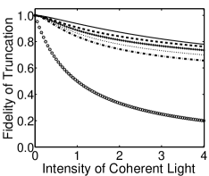
FIG. 5.: Effect of intensity of the input coherent light, $|\alpha|^{2}$, on the fidelity of truncation (left) and the number of coincidence and anticoincidence (C-AC) detections per second (right) when CPC’s with $R_{\rm dark}=100~{}{\rm s}^{-1}$ are used and $\gamma^{2}=5\times 10^{-4}/$pulse. In the left plot, $\eta=1.0,~{}0.7,~{}0.5,~{}0.3,~{}0.1$, and $0.0$ from top to bottom, respectively. In the right plot, $\eta=0.3,~{}0.5,~{}0.7$, and $1.0$ for $a,b,c$, and $d$, respectively.

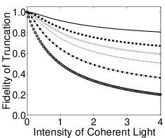
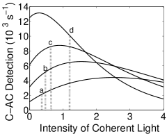
FIG. 6.: Effect of intensity of the input coherent light, $|\alpha|^{2}$, on the fidelity of truncation (left) and the number of coincidence and anticoincidence (C-AC) detections per second (right) when SPC’s with $R_{\rm dark}=10^{4}~{}{\rm s}^{-1}$ are used and $\gamma^{2}=5\times 10^{-4}$/pulse. In the left plot, $\eta=1.0,~{}0.7,~{}0.5,~{}0.3,~{}0.1$, and $0.0$ from top to bottom, respectively. In the right plot, $\eta=0.3,~{}0.5,~{}0.7$, and $1.0$ for $a,~{}b,~{}c$, and $d$, respectively.

number will drop to less than four states per second, and for higher intensities it will increase to up to $4000~{}{\rm s}^{2}{-1}$ but with much lower fidelities of around $0.6$.

4 Discussion of different detection strategies

In the analysis of CPC and SPC above, we have observed that CPC has the advantage of low dark count over SPC, however, SPC has the ability to discriminate between zero, one and more photons from each other. The best results would have been obtained, if we had photon counters combining these two advantages. Unfortunately, the current level of technology does not provide this to experimenters. However, in our QSD scheme, we can use a combination of CPC and SPC to benefit from their unique advantages. Simulations, with $R_{\rm dark}=100~{}{\rm s}^{-1}$ and $R_{\rm dark}=10^{4}~{}{\rm s}^{-1}$ for CPC and SPC, respectively, and $\eta=0.7$ for both, have shown that the choice of either CPC or SPC for $D_{3}$ does not cause a change at the fidelity of the output state. This can be easily understood by examining the $\Pi_{0}$ of the detectors. Dark count for $D_{3}$ shows itself as $e^{-\nu}$, which takes the value of $\cong 1$ for both CPC and SPC, resulting in the same value for fidelity. Therefore, we have only four different strategies for detector choice as shown in Table I.

In Fig. 7, it is seen that, for $0\leq|\alpha|^{2}\leq 4$, higher fidelity values are obtained for strategies $a$ and $b$, which use CPC’s as the “gating detector” $D_{1}$ and much lower ones are obtained for $c$ and $d$, which use SPC’s as $D_{1}$. We explain this as follows: Probability $P_{\rm real}$ of detecting a “click” at $D_{1}$ caused by real photons coming from SPDC is $O(\gamma^{2})$ per pulse, and the probability of a “click” caused by a dark count is $P_{\rm dark}=O(\nu)$. Then the condition that a “click” is caused by a real photon rather than a dark count can be written as $P_{\rm real}\gg P_{\rm dark}$, which implies $\nu\ll\gamma^{2}$. In the simulations, we used a coincidence window of 10 ns and $\gamma^{2}$ of order $\simeq 10^{-4}$/pulse. Then CPC has $\nu=10^{-6}$, which satisfies the above condition. SPC has $\nu=10^{-4}\approx\gamma^{2}$, which means that if an SPC is used for $D_{1}$ with coincidence window of 10 ns, there will be wrong triggerings and these will reflect themselves as decrease in fidelity. The parameter $\gamma^{2}$ has a profound effect on the fidelity of truncation for the four strategies.

Strategy	$D_{1}$	$D_{2}$	$D_{3}$
a	CPC	SPC	SPC or CPC
b	CPC	CPC	SPC or CPC
c	SPC	SPC	SPC or CPC
d	SPC	CPC	SPC or CPC

TABLE I.: Different strategies of detector choice for a realizable QSD. CPC, conventional photon counter; SPC, single-photon counter; $D_{1}$, gating detector; $D_{2}$ and $D_{3}$, detectors counting one and zero photons, respectively.

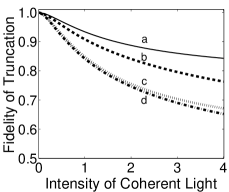
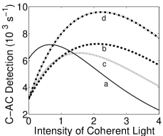
FIG. 7.: Effect of intensity of the input coherent light on the fidelity of truncation (left) and the number of coincidence and anticoincidence (C-AC) detections per second (right) for different strategies of detector choice.

Increasing the probability of generating single-photon pair from SPDC will increase the fidelity of truncation for those strategies where SPC is used as $D_{1}$ and decrease that of CPC. This is because the increasing values of $\gamma^{2}$ beyond $\nu\simeq 10^{-4}$ for SPC will diminish the dark count effects.

Moreover, SPC can distinguish the number of incident photons, which will lower the probability of a “false alarm” due to the generation of two or more photon pairs. On the other hand, in case of CPC, there will be “false alarms” that will reduce fidelity.

For $|\alpha|^{2}\leq 0.6$, fidelity $F$ is $>0.90$ for all strategies with a proper detection rate of ${\cal O}(10^{3}~{}{\rm s}^{-1})$. Then for truncating a low-intensity coherent state to prepare the desired superposition of vacuum and single-photon states, one can use CPC, because with a low intensity it is guaranteed that the number of photons in the system is less than two photons during a single preparation phase, and this will decrease the probability of having “false alarms” from $D_{2}$ and $D_{3}$. By contrast, if a strong light is used then we will have “clicks” at $D_{2}$ and $D_{3}$ when single or higher number of photons are incident on them, and since we cannot get information on the number of photons, we will still consider them as a sign of the desired truncation process, which will most of the time not be true.

V Comparison of fidelities for different states

An ideal perfect QSD scheme allows the truncation of a coherent state up to its single-photon state with $F=1$ conserving the relative phase and amplitude information. In an experimental realization, $F=1$ cannot be achieved due to error sources discussed in Sec. IV and fidelity depends strongly on the intensity of the input coherent light. One can always ask whether the fidelity values close to those obtained for the states generated with the experimental scheme can be obtained for some other states and how the state

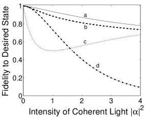
FIG. 8.: Comparison of fidelity of various states to the desired state $\sqrt{N}(|0\rangle+\alpha|1\rangle)$ with the normalization constant $N$. a, State obtained from experimental scheme with $\eta=1$; b, $\eta=0.5$ (dotted curve); c, $N(|0\rangle\langle 0|+|\alpha|^{2}|1\rangle\langle 1|)$; and d, coherent state $|\beta\rangle$ with $\alpha=\beta$.

prepared by QSD differs from those states. We will study two cases: (i) complete loss of phase information during the truncation process, which will yield the state $N(|0\rangle\langle 0|+|\alpha|^{2}|1\rangle\langle 1|)$, where $N$ is the normalization constant $1/(1+|\alpha|^{2})$ and (ii) a coherent state obtained by attenuating the input $|\alpha\rangle$,

$$|\beta\rangle=\big{|}\sqrt{\xi}~{}\alpha\big{\rangle},$$ (31)

which will be sent directly to the output without going through the truncation process of the QSD. Fidelities of these states to the desired state $\sqrt{N}(|0\rangle+\alpha|1\rangle)$ are found as

$$F_{1} = \frac{1+|\alpha|^{4}}{[1+|\alpha|^{2}]^{2}}\,,$$ (32)

$$F_{2} = \frac{e^{-|\beta|^{2}}}{1+|\alpha|^{2}}(1+2|\alpha\beta|\cos\Delta+|\alpha\beta|^{2}),$$ (33)

where $\Delta$ is the difference of arguments of the input coherent light $\alpha$ to be truncated and the coherent light of $\beta$. The optimum value for $\beta$ to obtain the maximum fidelity to the desired state for any $\alpha$ that is input to the QSD can be found as

$$|\beta|^{2} = \xi|\alpha|^{2}=\frac{1+2|\alpha|^{2}-\sqrt{1+4|\alpha|^{2}}}{2|\alpha|^{2}}\,,$$ (34)

$$\arg(\beta) = \arg(\alpha).$$ (36)

In Figs. 8 and 9, we have depicted the fidelities for these cases together with those of the states obtained from the proposed experimental scheme for $0\leq|\alpha|^{2}\leq 4$. With a perfect QSD scheme and correct information of one “click” at $D_{2}$ and no “click” at $D_{3}$, fidelity is one for any $|\alpha|^{2}$. For the state given in case (i), $F_{1}$ decreases gradually from $1.0$ to $0.5$ for $0\leq|\alpha|^{2}\leq 1.0$ and then starts increasing from $0.5$ at $|\alpha|^{2}=1.0$ to $0.68$ at $|\alpha|^{2}=4.0$. For the proposed scheme with CPC’s as the photon-counting detectors, fidelity

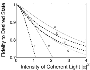
FIG. 9.: Comparison of the fidelity of the states obtained from the proposed experimental scheme of CPC’s with a, $\eta=1.0$; b, $\eta=0.7$; and c, $\eta=0.5$ with the fidelity of $|\beta\rangle$ of d, the optimized $\beta$ given by Eq. (34); e, $|\beta\rangle$ with $\xi=1/2$; and f, $|\beta\rangle$ with $\xi=1$.

of truncation is always higher than the fidelity values of case (i) in this range of $|\alpha|^{2}$ provided that $\eta\geq 0.5$. For the state given in case (ii), the fidelity for the optimized value of $\beta$ given by Eq. (34) is shown in Fig. 9 as curve d. The states prepared with the experimental QSD scheme have higher fidelity than the optimized $|\beta\rangle$ for $|\alpha|^{2}\geq 0.4$ at $\eta\geq 0.7$. This can be observed even for much lower $\eta$ at higher values of $|\alpha|^{2}$, i.e., for $|\alpha|^{2}>1.5$, $\eta=0.5$ is enough for the experimental scheme to have better fidelity. For some values of $\xi$ such as $\xi=1/2$ and $\xi=1$, the $|\beta\rangle$ states may have better fidelity for low $|\alpha|^{2}$. However, with increasing $|\alpha|^{2}$, there is a sharp monotonic decrease in their fidelities, which finally become very close to zero ($<0.09$) for $|\alpha|^{2}>4$. As a result, we can say that the proposed experimental scheme is more advantageous than the other strategies, because the states generated by the experimental scheme have higher fidelity for a broad range of $|\alpha|^{2}$ and $\eta$. In a limited range of low $|\alpha|^{2}$, other strategies may be optimized to give better fidelity, but only with the cost of much lower fidelity outside this range. As we will discuss in the next section, an analysis of the quasidistributions of those states will give us further information to discriminate those states from each other and to evaluate the efficiency and the merit of using the QSD scheme.

VI Quasidistributions for the Truncated Output State

In the previous section, to evaluate the QSD scheme, we have used fidelity to quantify how close the generated output state and the desired state are. However, fidelity is just a single number and does not give complete information on how well the phase and amplitude of the input to the QSD are preserved at the output. To answer this question we use the Wigner function as a tool since it is a one-to-one representation of the quantum state and contains all the information on state. In the following, the Wigner function is calculated as (see, e.g., [22])

$$W(X,P)=\frac{1}{\pi}\sum_{m,n}\rho_{mn}~{}\langle{n}|\hat{T}(X,P)|m\rangle,$$ (37)

where

$$\langle{n}|\hat{T}(X,P)|m\rangle = (-1)^{n}~{}2^{m-n+1}\,(X-{\rm i}P)^{m-n}\sqrt{\frac{n!}{m!}}$$ (39)

$$\times\exp(-2r^{2})~{}L_{n}^{m-n}(4r^{2})$$

with $r^{2}=X^{2}+P^{2}$, $L_{n}^{m-n}(y)$ being the associated Laguerre polynomial.

One of the most interesting characteristics of the QSD scheme is the generation of nonclassical states from a classical state. Negative values in the Wigner function are a sign of the nonclassical property of a state. Figure 10 shows the Wigner functions of the desired superposition state and the generated output state using the proposed experimental scheme with CPC’s as the photon-counting detectors. It is understood that even for $\eta=0.5$, the aim of generating a nonclassical state is achieved, however, we can argue that the information content (amplitude and relative phase) of the input state is partially lost during the truncation process due to the losses in the system. With decreasing $\eta$, the negativity in $W(X,P)$ becomes smaller and it is completely lost with further decrease beyond $\eta<0.4$.

If one considers the use of the optimized $|\beta\rangle$ state given by Eq. (34) rather than the QSD scheme to generate a state with the highest fidelity to the desired state of the form $\sqrt{N}(|0\rangle+\alpha|1\rangle)$ with $|\alpha|^{2}=0.8$ as in Fig. 10, an attenuation of $\xi\sim 0.43$, which will give an intensity of $|\beta|^{2}\sim 0.34$, must be used. In that case, fidelity to the desired state will be $0.92$, which is higher than the fidelity value of $F\sim 0.91$ obtained at $\eta=0.5$ and slightly lower than $F\sim 0.93$ obtained at $\eta=0.7$ if the proposed experimental scheme with CPC’s is used. Looking at only the values of fidelity of those states, one can conclude that it is difficult to discriminate these states from each other and may underestimate the advantage of using the QSD scheme. However, if the Wigner functions of those states are compared, the difference will become clearer. The Wigner function for $|\beta\rangle$ with $|\beta|^{2}\sim 0.34$ will be similar to Gaussian $W(X,P)$ for a coherent state with the peak located at $\sim 0.34$7 and having a circular symmetry where one cannot observe the negativity and the deformation seen in the desired state given in Fig. 10(a). On the other hand, although the fidelity values are very close to those of $|\beta\rangle$, the states generated by the QSD scheme have deformation and negativity similar to that of the desired state as seen in Fig. 10(b).

There is a delicate balance between the intensity of the coherent light and the efficiency of detectors to observe the negativity in $W(X,P)$. To show this clearly, we have analyzed marginal distributions and cross sections

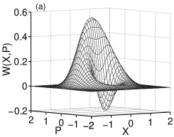
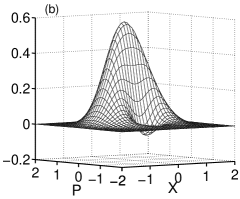
FIG. 10.: Wigner function for superpositions of vacuum and single-photon states obtained by truncating coherent state $|\alpha\rangle$ with $|\alpha|^{2}=0.8$ and phase $\pi/2$ using (a) the perfect QSD and (b) proposed experimental scheme with CPC’s for $\eta=0.7$, $R_{\rm dark}=100~{}{\rm s}^{-1}$, and $\gamma^{2}=5\times 10^{-4}$/pulse.

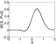
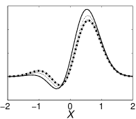
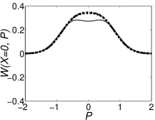
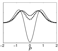
FIG. 11.: Effect of detector efficiency on Wigner function of the output states generated by truncating coherent states of different intensities: $|\alpha|^{2}=0.4$ (left) and $|\alpha|^{2}=4.0$ (right figures). Solid curve is for the perfect QSD, and dash-dotted, dotted, and dashed curves are for $\eta=0.5,0.7$, and $1$, respectively.

of Wigner functions for different $|\alpha|^{2}$ and $\eta$ and depicted some results in Figs. 11. We have understood that for coherent input of low intensity $|\alpha|^{2}<1.0$, detector losses and source imperfections do not have a significant effect on the shape of the Wigner function. For $\eta\geq 0.4$, the shape of the Wigner function and marginal probabilities of the states obtained from the proposed scheme and the desired state are almost the same. For the range $1.0\leq|\alpha|^{2}\leq 1.5$, negativity in $W(X,P=0)$ can be observed for $\eta\geq 0.2$, however, $W(X=0,P)$ becomes smoothed and the dip seen in the ideal case fades with decreasing $\eta$. For $|\alpha|^{2}>1.5$, the effect of detector efficiency is more profound. Moreover, it affects $W(X,P=0)$ and $W(X=0,P)$ differently. For decreasing $\eta$, although the value of negativity in $W(X,P=0)$ approaches zero, the negativity can still be observed for $\eta>0.3$. On the other hand, the dip

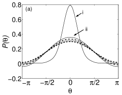
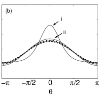
FIG. 12.: Wigner phase distributions $P(\theta)$ of truncated output states obtained from input coherent states of (a) $|\alpha|^{2}=1.0$ and (b) $|\alpha|^{2}=0.4$. Solid curves labeled as $(i)$ and $(ii)$ denote the phase distributions of the input coherent states and the truncated output states with the perfect QSD, respectively. Results of the proposed scheme are shown as dash-dotted, dotted, and dashed curves for $\eta=1.0,~{}0.5$, and $0.2$, respectively.

seen in $W(X=0,P)$ is strongly smoothed monotonically with increasing efficiency. Strong dips similar to the ideal case can be observed for $0.2<\eta<0.5$. This deformation in the Wigner function of the output state for high intensity input coherent lights can be explained with the intrinsic property of the CPC’s, that is, they lose the information on the number of incident photons. For strong lights, the number of photons in the system will be higher than two photons, which will trigger “false alarms” about the generation of the desired state causing strong deformations in the Wigner function.

Another important point of the QSD scheme is the preservation of the relative phase between vacuum and single-photon components in the ideal case, so it is necessary to study the phase and its distribution for the output state. The effect of imperfections on the phase distribution of the generated state is analyzed using Wigner phase distribution, which is the phase distribution associated with the Wigner function and calculated using [22]

$$P(\theta)=\int_{0}^{\infty}W(\beta)|\beta|d|\beta|\,,$$ (40)

where $W(\beta)$ can be obtained from Eqs. (37)–(39) using $\beta=X+{\rm i}P$.

Analysis of Wigner phase distribution for different intensities of the input coherent light and different detector efficiencies has revealed the following.

(i) Maximum value of the phase distribution is obtained at the phase of the input coherent light, which implies that the preferred phase for the output state obtained from the experimental scheme is the phase of the input light. It must be noted that in the proposed model we have not included phase-dependent losses.

(ii) Low detector efficiency and losses in the system smooth and broaden the phase distribution. In the limit $\eta=0$, phase distribution is flat and $P(\theta_{1})\sim 0.1592$, which are also observed for the vacuum state.

(iii) For $0.25<|\alpha|^{2}<0.45$, phase distribution has negativity for the ideal scheme. To preserve the negativity of phase distribution in the experimental scheme, detector efficiency must be high, i.e., for $|\alpha|^{2}=0.4,1.0$, and $2.0$, detector efficiency $\eta$ must be greater than $0.9,0.6$, and $0.7$, respectively. However, the minimum value of $P(\theta)$ is much higher than that of the ideal case even for $\eta=1$.

(iv) Negativity of the Wigner phase distribution can be preserved with $\eta\geq 0.65$ when the weights of the vacuum and single-photon states are comparable (nearly equal), because the minimum of the phase distribution is more strongly negative for these cases, i.e., in the ideal case, $|\alpha|^{2}=1$ and the unnormalized state $|0\rangle+\alpha|1\rangle$, $P(\theta_{1})$ becomes $\sim-0.0403$, which is the lowest minimum for any $|\alpha|^{2}$ for this superposition state. Figure 12 shows the effect of detector efficiency on the Wigner phase distribution for input states of different intensities.

VII CONCLUSIONS

In this study, we have analyzed the QSD scheme proposed by Pegg et al. in detail using realistic descriptions for the detectors and single-photon source. We have also proposed and discussed a simple and realizable experimental scheme for the QSD considering possible error sources that can be encountered in practice. The possible ways of solving these difficulties and their effect on the generated output state are discussed. We have shown explicitly that the proposed scheme is realizable with high fidelity using commercially available detectors and SPDC as the single-photon source. With a further analysis using quasidistributions, it has been clarified that the states prepared with the QSD scheme have nonclassical properties, and one can distinguish these states from states generated by other strategies. Moreover, it has been shown that the value of the preferred relative phase between the vacuum and single-photon states of the input coherent light is preserved at the truncated output state. The verification of truncation process can be done using a combination of photon counting and homodyning or by more sophisticated methods such as homodyne-tomography techniques [23].

to appear in Phys. Rev. A 64, 0638xx (2001)