Simulation and reversal of $n$-qubit Hamiltonians using Hadamard matrices

Abstract

The ability to simulate one Hamiltonian with another is an important primitive in quantum information processing. In this paper, a simulation method for arbitrary $\sigma_{z}\otimes\sigma_{z}$ interaction based on Hadamard matrices (quant-ph/9904100) is generalized for any pairwise interaction. We describe two applications of the generalized framework. First, we obtain a class of protocols for selecting an arbitrary interaction term in an $n$-qubit Hamiltonian. This class includes the scheme given in quant-ph/0106064v2. Second, we obtain a class of protocols for inverting an arbitrary, possibly unknown $n$-qubit Hamiltonian, generalizing the result in quant-ph/0106085v1.

I Introduction

An important element in quantum information processing is the ability to efficiently convert a set of primitives, determined by the physical system, to perform the desired task. In many physical systems, the primitives are “local manipulations” such as fast single qubit operations that can easily be controlled, and a given nonlocal system Hamiltonian that cannot be changed. In this case, the desired task may be approximated or simulated by interspersing the given Hamiltonian evolution with local manipulations. The resources of simulation include the amount of local manipulations and the total operation time of the given Hamiltonian.

Such simulation was extensively studied in the context of NMR quantum computation [1, 2, 3] in which the naturally occurring Hamiltonian cannot be controlled. Reference [2] presents a method based on Hadamard matrices to convert the evolution due to any Hamiltonian of the form

$$H_{1}=\sum_{i<j}g_{ij}\,\sigma_{z}^{(i)}\otimes\sigma_{z}^{(j)}+\sum_{i}\omega_{i}\,\sigma_{z}^{(i)}$$ (1)

to that of a particular term $g_{lm}\sigma_{z}^{(l)}\otimes\sigma_{z}^{(m)}$ where $\sigma_{z}^{(i)}$ is a Pauli matrix acting on the $i$-th qubit. The same protocol applies universally for all coefficients $g_{ij}$ and $\omega_{i}$. Other arbitrary evolutions can in turns be obtained by reduction to the universality construction [4, 5, 6]. The simulation of the single term is exact, and does not require frequent local manipulations. A related task to stop the interaction is also addressed. The method aims at minimizing the amount of local operations, measured by the number of interval of free evolution or the number of single qubit gates required.

A more general problem was addressed recently in Ref. [7]. A major step is to convert the Hamiltonian

$$H_{2}=\sum_{ij}\sum_{\alpha\beta}g_{ij\alpha\beta}\,\sigma_{\alpha}^{(i)}\otimes\sigma_{\beta}^{(j)}+\sum_{i}\vec{r}^{\,(i)}\cdot\vec{\sigma}^{(i)}$$ (2)

to a single term $g_{lm\gamma\eta}\sigma_{\gamma}^{(l)}\otimes\sigma_{\eta}^{(m)}$, where $\sigma_{\alpha=x,y,z}$ denote the Pauli matrices. The single term is then used to simulate the dynamics due to any other Hamiltonian

$$H_{2}^{\prime}=\sum_{ij}\sum_{\alpha\beta}g^{\prime}_{ij\alpha\beta}\,\sigma_{\alpha}^{(i)}\otimes\sigma_{\beta}^{(j)}+\sum_{i}\vec{r}\,^{\prime(i)}\cdot\vec{\sigma}^{(i)}$$ (3)

For each required accuracy level, both local and nonlocal resources are analyzed.

Related problems were also discussed in Refs. [8, 9], focusing on more specific types of given Hamiltonians and the operation time for the simulation. Bounds are derived for the operation time to use

$$H_{3}=\sum_{ij}\sigma_{z}^{(i)}\otimes\sigma_{z}^{(j)}$$ (4)

to simulate an arbitrary Hamiltonian $H^{\prime}_{2}$ given by Eq. (3). Methods and the required operating times for a Hamiltonian $H$ to simulate its inverse evolution $e^{iHt}$ are also studied. This is done for the Hamiltonians $H_{3}$ in Eq. (4) and $H_{4}$ given by

$$H_{4}=\sum_{\alpha}d_{\alpha}\sum_{ij}\sigma_{\alpha}^{(i)}\otimes\sigma_{\alpha}^{(j)}$$ (5)

which is essentially the most general Hamiltonian for pairwise interaction with permutation symmetry.

The general principle in these simulation schemes is to transform some coupling terms to the desired form and to cancel out the rest, by interspersing the free evolution with single qubit operations. In this paper, we generalize the framework developed in Ref. [2] to apply to the more general given Hamiltonian in Eq. (2). Using this framework, we find a class of schemes that select a term $\sigma_{\gamma}^{(l)}\otimes\sigma_{\eta}^{(m)}$ from a Hamiltonian given by Eq. (2). This class of schemes includes the method presented in Ref. [7]. We also consider time reversal using the generalized framework, and present a class of protocols to reverse an arbitrary Hamiltonian given by Eq. (2). They require an operation time $c3nt$ of $H_{2}$ to simulate the reversed evolution $e^{iH_{2}t}$ where $1\leq c\leq 2$ and $c\approx 1$ for large $n$. The schemes are designed to be independent of the given Hamiltonian, and are applicable even when $H_{2}$ is unknown. This generalizes the results in Ref. [9].

After the initial submission of this paper, related work were independently reported in Ref. [11]. Methods to stop the evolution due to a Hamiltonian given by Eq. (2), and to select all diagonal coupling terms between a designated pair of qubits are given. Simplifications for diagonal couplings and higher order terms were considered. Our framework to stop the evolution is closely related to, but subtly different from that in Ref. [11], and allows more flexibility in selecting coupling terms, such as the selection of any single interaction term. We are also interested in a tighter bound on the required local resources, and in the inversion of Hamiltonians.

This paper is structured as follows. In Section II, we review the framework and various resulting schemes in Ref. [2], with a slight change from the original NMR based notations. The framework is generalized for any Hamiltonian given by Eq. (2) in Section III. The first application to select individual coupling terms from the given Hamiltonian is discussed in Section IV. The second application to simulate time reversal is discussed in Section V as a simple application. The technical details of the construction are described in Appendices A and B.

II Selective coupling using Hadamard matrices – a review

A Statement of the problem

We review the method developed in Ref. [2]. Consider an $n$-qubit system, evolved according to the Hamiltonian

$$H_{z}=\sum_{i<j}g_{ij}\sigma_{z}^{(i)}\otimes\sigma_{z}^{(j)}\,,$$ (6)

where $g_{ij}$ are arbitrary coupling constants. The goal is to evolve the system according to only one term of the Hamiltonian:

$$\sigma_{z}^{(i)}\otimes\sigma_{z}^{(j)}\,,$$ (7)

using single qubit operations. We call this task “selective coupling.” This is closely related to the task of stopping the evolution or “decoupling.” We first develop a framework for decoupling. Then we construct decoupling and selective coupling schemes using Hadamard matrices.

B Decoupling scheme for two qubits

We motivate the general construction using the simplest example of decoupling two qubits. Let $U_{t}=e^{-iH_{z}t}$, where the Hamiltonian is given by $H_{z}=g_{12}\,t\,\sigma_{z}^{(1)}\!\otimes\sigma_{z}^{(2)}$. We use the shorthand $X^{(i)}$ for $\sigma_{x}^{(i)}$. We also use the important identity

$$Ue^{M}U^{\dagger}=e^{UMU^{\dagger}}$$ (8)

where $M$ is any bounded square matrix and $U$ is any unitary matrix of the same dimension. As the Pauli matrices anticommute,

$$X^{(2)}\,U_{t}\,X^{(2)} = X^{(2)}\;e^{-i\,g_{12}\,t~{}\sigma_{z}^{(1)}\otimes\,\sigma_{z}^{(2)}}X^{(2)}$$ (9)

$$= e^{-i\,g_{12}\,t~{}\sigma_{z}^{(1)}\otimes\,(X^{(2)}\sigma_{z}^{(2)}X^{(2)})}$$ (10)

$$= e^{-i\,g_{12}\,t~{}\sigma_{z}^{(1)}\otimes\,(-\sigma_{z}^{(2)})}~{}~{}=~{}~{}U_{t}^{-1}$$ (11)

Thus adding the gate $X^{(2)}$ before and after the free evolution reverses it, and

$$X^{(2)}\,U_{t}\,X^{(2)}\,U_{t}=I\,.$$ (12)

This illustrates how single qubit operations can transform the action of one Hamiltonian to another.

Equation (12) can be written to highlight some essential features leading to decoupling:

$$e^{-i\,g_{12}\,t\,(+\sigma_{z}^{(1)})\otimes(-\sigma_{z}^{(2)})}\times e^{-i\,g_{12}\,t\,(+\sigma_{z}^{(1)})\otimes(+\sigma_{z}^{(2)})}\,.$$ (13)

Each factor corresponds to a “time interval” of evolution.
1. In each interval, each $\sigma_{z}^{(i)}$ acquires a $-$ or $+$ sign, according to whether $X^{(i)}$ are applied or not before and after the time interval.
2. The bilinear coupling is unchanged (negated) when the signs of $\sigma_{z}^{(1)}$ and $\sigma_{z}^{(2)}$ agree (disagree).
3. Since the matrix exponents commute, negating the coupling for exactly half of the total time is necessary and sufficient to cancel out the coupling.

The crucial point leading to decoupling is that, the signs of the $\sigma_{z}$ matrices of the coupled qubits, controlled by the $X$ gates, disagree for half of the total time elapsed.

C Sign matrix and decoupling criteria

We now generalize the framework for decoupling to $n$ qubits. Each of our schemes concatenates some $m$ equal-time intervals. In each time interval, the sign of each $\sigma_{z}^{(i)}$ can be $+$ or $-$ as controlled by the $X$ gates. Each scheme is specified by an $n\times m$ “sign matrix”, with the $(i,a)$ entry being the sign of $\sigma_{z}^{(i)}$ in the $a$-th time interval. The entries in each column represent the signs of all the qubits at the corresponding time interval and the entries in each row represents the time sequence of signs for the corresponding qubit. We denote a sign matrix for $n$ qubits by $S_{n}$. For example, the scheme in Eq. (13) can be represented by the sign matrix

$$S_{2}=\left[\begin{array}[]{cc}{+}&{+}\\ {+}&{-}\end{array}\right]\,.$$ (14)

Following the discussion in Sec. II B, we have

Decoupling criteria – version 1    Decoupling is achieved if any two rows in the sign matrix disagree in exactly half of the entries.

For example, the following sign matrix decouples four qubits:

$$S_{4}=\left[\begin{array}[]{cccc}{+}&{+}&{+}&{+}\\ {+}&{+}&{-}&{-}\\ {+}&{-}&{-}&{+}\\ {+}&{-}&{+}&{-}\end{array}\right]\,.$$ (15)

More explicit, the scheme is given by

$$U_{t}\times(X^{(3)}X^{(4)}\,U_{t}\,X^{(3)}X^{(4)})~{}\times\hskip 81.8053pt$$ (16)

$$~{}(X^{(2)}X^{(3)}\,U_{t}\,X^{(2)}X^{(3)})\times(X^{(2)}X^{(4)}\,U_{t}\,X^{(2)}X^{(4)})\,,$$ (17)

where $U_{t}=e^{-iH_{z}t}$ has six possible coupling terms in the $4$-qubit Hamiltonian. The relation between the scheme and $S_{4}$ is illustrated in Figure 1.

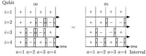
FIG. 1.: (a) Converting the sign matrix $S_{4}$ to the scheme in Eq. (16). A “$-$” sign in the $i$-th row and $a$-th column translates to $X^{(i)}$ (acting on the $i$-th qubit) before and after the $a$-th time interval. (b) Simplifying the scheme using $X^{(i)}X^{(i)}=I$.

From now on, we only consider the sign matrices, which completely represent the corresponding schemes. For $n$ qubits when $n$ is large, $n\times m$ sign matrices with small $m$ can be difficult to construct. For example,

$$S_{n}=\left[\begin{array}[]{cccccccccccc}{+}&{\cdots}&{+}&{+}&{\cdots}&{+}&{+}&{\cdots}&{+}&{+}&{\cdots}&{+}\\ {+}&{\cdots}&{+}&{+}&{\cdots}&{+}&{-}&{\cdots}&{-}&{-}&{\cdots}&{-}\\ {+}&{\cdots}&{+}&{-}&{\cdots}&{-}&{+}&{\cdots}&{+}&{-}&{\cdots}&{-}\\ {}\hfil&{\cdots}&{}\hfil&{}\hfil&{\cdots}&{}\hfil&{}\hfil&{\cdots}&{}\hfil&{}\hfil&{\cdots}&{}\hfil\\ {}\hfil&{\cdots}&{}\hfil&{}\hfil&{\cdots}&{}\hfil&{}\hfil&{\cdots}&{}\hfil&{}\hfil&{\cdots}&{}\hfil\\ {+}&{-~{}+}&{-}&{+}&{-~{}+}&{-}&{+}&{-~{}+}&{-}&{+}&{-~{}+}&{-}\end{array}\right]\,,$$ (24)

in which an interval from a previous row is bifurcated takes $m=2^{n-1}$. As the number of columns represents local resources for the simulation, our goal is to find solutions with the smallest number of columns. We solve this problem by first rephrasing the decoupling criteria:

Decoupling criteria – version 2   Identifying $\pm$ with $\pm 1$ in $S_{n}$, decoupling is achieved if any two rows have zero inner product, or $S_{n}S_{n}^{T}=nI$.

We now present very efficient solutions to the decoupling criteria, which are derived from the Hadamard matrices [12, 13, 14, 15].

D Hadamard matrices and decoupling scheme

A Hadamard matrix of order $n$, denoted by $H(n)$, is an $n\times n$ matrix with entries $\pm 1$, such that

$$H(n)H(n)^{T}=nI\,.$$ (25)

Thus every $H(n)$, if exists, is a valid sign matrix corresponding to a decoupling scheme for $n$ qubits using only $n$ time intervals. The following is a list of interesting facts about Hadamard matrices (see Refs. [12, 13, 14, 15] for details and proofs).

1. Equivalence  Any permutation, or negation of any row or column of a Hadamard matrix preserves the orthogonality condition. Thus each Hadamard matrix can be transformed to a normalized one, which has only $+$’s in the first row and column.

2. Necessary conditions  $H(n)$ exists only for $n=1$, $n=2$ or $n\equiv 0\bmod 4$.

3. Hadamard’s conjecture [16]  $H(n)$ exists for every $n\equiv 0\bmod 4$. This famous conjecture is verified for all $n<428$.

4. Sylvester’s construction [17]  If $H(n)$ and $H(m)$ exist, then $H(n)\otimes H(m)$ is a possible $H(nm)$. In particular, $H(2^{r})$ can be constructed as $H(2)^{\otimes r}$, which is proportional to the matrix representation of the Hadamard transformation for $r$ qubits.

5. Paley’s construction [18]  Let $q$ be an odd prime power. If $q\equiv 3\bmod 4$, then $H(q\!+\!1)$ exists; if $q\equiv 1\bmod 4$, then $H(2(q\!+\!1))$ exists.

6. Numerical facts [12]   For an arbitrary integer $n$, let $\overline{n}$ be the smallest integer satisfying $n\leq\overline{n}$ with known $H(\overline{n})$. For $n\leq 1000$, $H(n)$ is known for every but $6$ possible orders, and $\overline{n}-n\leq 7$. For $n\leq 10000$, $H(n)$ is unknown for only $192$ possible orders and $\overline{n}-n\leq 31$.

The nontrivial existence of so many Hadamard matrices may be better appreciated by examining the following example of $H(12)$, obtained with Paley’s construction.

$$H(12)=\left[\begin{array}[]{cccccccccccc}{+}&{+}&{+}&{+}&{+}&{+}&{+}&{+}&{+}&{+}&{+}&{+}\\ {+}&{+}&{+}&{-}&{-}&{+}&{-}&{-}&{+}&{-}&{-}&{+}\\ {+}&{+}&{+}&{+}&{-}&{-}&{-}&{+}&{-}&{+}&{-}&{-}\\ {+}&{-}&{+}&{+}&{+}&{-}&{-}&{-}&{+}&{-}&{+}&{-}\\ {+}&{-}&{-}&{+}&{+}&{+}&{-}&{-}&{-}&{+}&{-}&{+}\\ {+}&{+}&{-}&{-}&{+}&{+}&{-}&{+}&{-}&{-}&{+}&{-}\\ {+}&{-}&{-}&{-}&{-}&{-}&{-}&{+}&{+}&{+}&{+}&{+}\\ {+}&{-}&{+}&{-}&{-}&{+}&{+}&{-}&{-}&{+}&{+}&{-}\\ {+}&{+}&{-}&{+}&{-}&{-}&{+}&{-}&{-}&{-}&{+}&{+}\\ {+}&{-}&{+}&{-}&{+}&{-}&{+}&{+}&{-}&{-}&{-}&{+}\\ {+}&{-}&{-}&{+}&{-}&{+}&{+}&{+}&{+}&{-}&{-}&{-}\\ {+}&{+}&{-}&{-}&{+}&{-}&{+}&{-}&{+}&{+}&{-}&{-}\end{array}\right]\,.$$ (38)

Thus there is a simple decoupling scheme for $n$ qubits if $H(n)$ exists. Using Hadamard matrices, decoupling and recoupling schemes for an arbitrary number of qubits can be easily constructed, as will be shown next.

E Decoupling and selective coupling

Decoupling    When an $H(n)$ exists, it corresponds to a decoupling scheme for $n$ qubits concatenating only $n$ time intervals. When an $H(n)$ does not necessarily exist, consider $H(\overline{n})$ and choose any $n$ rows to form an $S_{n}$. Then $S_{n}$ corresponds to a decoupling scheme for $n$ qubits requiring $\overline{n}$ time intervals. As an example, $S_{9}$ can be chosen to be the first nine rows of $H(12)$ in Eq. (38):

$$S_{9}=\left[\begin{array}[]{cccccccccccc}{+}&{+}&{+}&{+}&{+}&{+}&{+}&{+}&{+}&{+}&{+}&{+}\\ {+}&{+}&{+}&{-}&{-}&{+}&{-}&{-}&{+}&{-}&{-}&{+}\\ {+}&{+}&{+}&{+}&{-}&{-}&{-}&{+}&{-}&{+}&{-}&{-}\\ {+}&{-}&{+}&{+}&{+}&{-}&{-}&{-}&{+}&{-}&{+}&{-}\\ {+}&{-}&{-}&{+}&{+}&{+}&{-}&{-}&{-}&{+}&{-}&{+}\\ {+}&{+}&{-}&{-}&{+}&{+}&{-}&{+}&{-}&{-}&{+}&{-}\\ {+}&{-}&{-}&{-}&{-}&{-}&{-}&{+}&{+}&{+}&{+}&{+}\\ {+}&{-}&{+}&{-}&{-}&{+}&{+}&{-}&{-}&{+}&{+}&{-}\\ {+}&{+}&{-}&{+}&{-}&{-}&{+}&{-}&{-}&{-}&{+}&{+}\end{array}\right]\,.$$ (48)

Selective coupling   To implement selective coupling between the $i$-th and the $j$-th qubits, any two rows in the sign matrix should be orthogonal, except for the $i$-th and $j$-th rows that are identical. The coupling $g_{ij}\;\sigma_{z}^{(i)}\otimes\sigma_{\rm z}^{(j)}$ acts all the time while all other couplings are canceled. The sign matrix can be obtained by taking $n-1$ rows from $H(\overline{n\!-\!1})$. For example, to couple the last two among $9$ qubits, we can take $S_{8}$ to be the $9\times 8$ matrix obtained from appending the last row of $H(8)$ to itself. Alternatively, we can take the $2$-nd to the $9$-th rows of $H(12)$ in Eq. (38), and repeat the last row:

$$S_{9}=\left[\begin{array}[]{cccccccccccc}{+}&{+}&{+}&{-}&{-}&{+}&{-}&{-}&{+}&{-}&{-}&{+}\\ {+}&{+}&{+}&{+}&{-}&{-}&{-}&{+}&{-}&{+}&{-}&{-}\\ {+}&{-}&{+}&{+}&{+}&{-}&{-}&{-}&{+}&{-}&{+}&{-}\\ {+}&{-}&{-}&{+}&{+}&{+}&{-}&{-}&{-}&{+}&{-}&{+}\\ {+}&{+}&{-}&{-}&{+}&{+}&{-}&{+}&{-}&{-}&{+}&{-}\\ {+}&{-}&{-}&{-}&{-}&{-}&{-}&{+}&{+}&{+}&{+}&{+}\\ {+}&{-}&{+}&{-}&{-}&{+}&{+}&{-}&{-}&{+}&{+}&{-}\\ {+}&{+}&{-}&{+}&{-}&{-}&{+}&{-}&{-}&{-}&{+}&{+}\\ {+}&{+}&{-}&{+}&{-}&{-}&{+}&{-}&{-}&{-}&{+}&{+}\end{array}\right]\,.$$ (58)

The extra feature of this $S_{9}$ is that, all row sums are zero. This is because $H(12)$ in Eq. (38) is normalized, so that all rows except for the first have zero row sums. This automatically removes any local (linear) terms $\sum_{i}\omega_{i}\sigma_{z}^{(i)}$ in the Hamiltonian, without extra local resources (see Ref. [2] for a full discussion). Finally, we note that coupling terms involving disjoint pairs of qubits can be selected simultaneously.

F Discussion

Upper bound on $\overline{n}$   For $n$ qubits, selective coupling requires at most $\overline{n}$ intervals and $n\overline{n}$ single qubit gates. In fact, $\overline{n}=cn$ where $c$ is very close to the ideal lower bound $c=1$. First, if Hadamard’s conjecture is proven, $\overline{n}$ only depends on $n\bmod 4$, and $\forall_{n}$ $\overline{n}\!-\!n\leq 3$. Even without this conjecture, the present knowledge in Hadamard matrices implies $\overline{n}\!-\!n\leq 8$ $\forall$ $n\leq 1000$, and $\overline{n}\!-\!n\leq 32$ $\forall$ $n\leq 10000$. A detailed proof for $c\approx 1$ for arbitrarily large $n$ is given in an Appendix of Ref. [2], while Sylvester’s construction puts an immediate loose bound of $c<2$.
Gate simulation vs dynamics simulation [10] The previous discussion assumes that the goal is to simulate the final unitary transformation due to the Hamiltonian $\sigma_{z}^{(i)}\!\otimes\sigma_{z}^{(j)}$ for time $t$. Due to the commutivity of all the possible coupling terms, we only need to divide the time into $\overline{n}$ time intervals, each with finite duration $t/\overline{n}$. On the other hand, if the goal is to simulate the dynamics due to $\sigma_{z}^{(i)}\!\otimes\sigma_{z}^{(j)}$ for time $t$, one should instead apply the scheme to simulate the unitary gate “$e^{-i\sigma_{z}^{(i)}\otimes\sigma_{z}^{(j)}\Delta t}$” $t/\Delta t$ times where $\Delta t$ is a small time interval. We will focus on simulating the dynamics of a Hamiltonian in the rest of the paper.

III Generalized framework for arbitrary $n$-qubit Hamiltonians

We now generalize the framework for a more general given Hamiltonian (Eq. (2)):

$$H_{2}=\sum_{ij}\sum_{\alpha\beta}g_{ij\alpha\beta}\,\sigma_{\alpha}^{(i)}\otimes\sigma_{\beta}^{(j)}+\sum_{i}\vec{r}^{\,(i)}\cdot\vec{\sigma}^{(i)}$$ (59)

The goal is again to simulate the evolution due to one specific coupling term $\sigma_{\gamma}^{(l)}\otimes\sigma_{\eta}^{(m)}$. Passing from Eq. (1) to Eq. (59), the first difference is the noncommutivity of the terms in Eq. (59). The second difference is the presence of all three Pauli matrices acting on the same qubit, besides a much larger number of coupling terms.

We adopt a common approach [7, 8, 10] that employs sufficiently frequent local manipulations to make the effect of the non-commutivity negligible. This is based on the identity

$$e^{-iK_{1}t_{1}}e^{-iK_{2}t_{2}}\approx e^{-i(K_{1}t_{1}+K_{2}t_{2})}+{\cal O}(t_{1}t_{2})\,,$$ (60)

which implies that effects of non-commutivity are of higher order in the small $t_{i}$ in Eq. (60). Thus the discussion proceeds neglecting the non-commutivity, and products of unitary evolutions are replaced by sums of the exponents. With this simplification, the framework in the previous section is readily generalized.

Again, we consider a class of schemes that concatenate (short) equal time intervals of evolution. The essential features for decoupling are as before:
1. In each interval, each $\sigma_{\alpha}^{(i)}$ acquires a $+$ or $-$ sign, which is controlled by the applied local unitaries to be described.
2. The bilinear coupling $g_{ij\alpha\beta}\,\sigma_{\alpha}^{(i)}\otimes\sigma_{\beta}^{(j)}$ for $i\neq j$ is unchanged (negated) when the signs of $\sigma_{\alpha}^{(i)}$ and $\sigma_{\beta}^{(j)}$ agree (disagree).
3. To the lowest order in the duration of the time intervals, negating a coupling for exactly half of the intervals cancels it.
The generalized framework differs from the original one [2] in that, the signs of the three Pauli matrices $\sigma_{\alpha=x,y,z}^{(i)}$ acting on the same qubit $i$ in the same time interval are not independent. In fact, the three signs multiply to $+$, because conjugating $\vec{r}^{\,(i)}\cdot\vec{\sigma}^{(i)}$ by (local) unitaries on the $i$-qubit transforms $\vec{r}^{\,(i)}$ by an SO(3) matrix. Conversely, any sign assignment satisfying this constraint can be realized. The possible signs for $\sigma_{x}^{(i)},\sigma_{y}^{(i)},\sigma_{z}^{(i)}$ are $+++$, $+--$, $-+-$, $--+$, and are realized by applying $I^{(i)}$, $\sigma_{x}^{(i)}$, $\sigma_{y}^{(i)}$, $\sigma_{z}^{(i)}$ respectively before and after the interval. Incorporating these considerations, we generalize the previous framework:

A scheme for $n$ qubits that concatenates $m$ intervals can be specified by three $n\times m$ sign matrices $S_{x}$, $S_{y}$, $S_{z}$, related by the entry-wise product $S_{x}\,\mbox{.{\fds*}\hskip 0.43057pt}S_{y}=S_{z}$. The $(i,a)$ entry of $S_{\alpha}$ is the sign of $\sigma_{\alpha}^{(i)}$ in the $a$-th time interval.

We omit the number of qubits, $n$, in $S_{x}$, $S_{y}$, $S_{z}$ for simplicity of notation. The entry-wise product .*  of two matrices is also known as the Schur product or the Hadamard product.

IV Selective coupling for $n$ qubits with arbitrary pairwise coupling

Under the generalized framework, we state the criteria for decoupling and selective coupling for $n$ qubits:

Criteria for decoupling and selective coupling    Decoupling is achieved if any two rows taken from $S_{x}$, $S_{y}$, $S_{z}$ are orthogonal. Selective coupling of $\sigma_{\gamma}^{(l)}\otimes\sigma_{\eta}^{(k)}$ is achieved if the $l$-th row of $S_{\gamma}$ is identical to the $k$-th row of $S_{\eta}$, but any other pair of rows from $S_{x}$, $S_{y}$, $S_{z}$ are orthogonal. Local terms are removed if all row sums are zero.

Sign matrices $S_{x,y,z}$ satisfying the criteria can be constructed from special Hadamard matrices endowed with certain extra structures. We now describe the constructions of the sign matrices, which elicit the special properties required of the starting Hadamard matrices. The more difficult and technical constructions of these special Hadamard matrices are given in detail in Appendices A and B.

Suppose we want to decouple $n$ qubits using a Hadamard matrix $H(m)$. The orthogonality condition is automatically satisfied if the rows of $S_{x,y,z}$ are taken to be distinct rows of $H(m)$. It remains to ensure $S_{x}\mbox{.{\fds*}\hskip 0.43057pt}S_{y}=S_{z}$. We call a set of $3$ vectors of equal length and with entries $\pm 1$ a Schur-set if they entry-wise multiply to $++\cdots+$. For example, $\{[+--],[-+-],[--+]\}$ is a Schur-set. If $H(m)$ has at least $3n$ rows that partition into $n$ Schur-subsets, one can ensure $S_{x}\mbox{.{\fds*}\hskip 0.43057pt}S_{y}=S_{z}$ by choosing the $i$-th rows of $S_{x},S_{y},S_{z}$ to be the rows of the $i$-th Schur-subset. This poses the first extra property on $H(m)$ – its rows partition into many Schur-subsets. Note the immediate lower bound on the size of $H(m)$, $\lfloor(m-1)/3\rfloor\geq n$ under this construction. This is not a strict lower bound, as a modification (to be described later) to the construction enables $n$ to be replaced by $n+1$, but the modification removes some useful properties.

Schemes for selective coupling can be derived from decoupling schemes as follows. Let $\{\gamma,\eta,\nu\}=\{x,y,z\}$ be distinct labels. To select the coupling $\sigma_{\gamma}^{(l)}\otimes\sigma_{\eta}^{(k)}$ one can modify the decoupling sign matrices as follows:

(61)

where $v_{\alpha}$, $w_{\alpha}$ for $\alpha\in\{\gamma,\eta,\nu\}$ denote the rows. To select the coupling $\sigma_{\gamma}^{(l)}\otimes\sigma_{\gamma}^{(k)}$, proceed as before and further swap the $k$-th rows of $S_{\gamma}$ and $S_{\eta}$ (these are $w_{\gamma}$ and $v_{\gamma}$ in the lower diagram). In both cases, it is necessary to ensure $w_{\gamma}\mbox{.{\fds*}\hskip 0.43057pt}v_{\gamma}$ is a row of $H(m)$ and is not used elsewhere in $S_{x,y,z}$. To ensure $w_{\gamma}\mbox{.{\fds*}\hskip 0.43057pt}v_{\gamma}$ is a row of $H(m)$, one poses a second special property in $H(m)$ that, it contains $5$ rows $f_{1,\cdots,5}$ such that

$$f_{1}\mbox{.{\fds*}\hskip 0.43057pt}f_{2}=f_{3}\mbox{.{\fds*}\hskip 0.43057pt}f_{4}=f_{5}\,.$$ (62)

Then we can simply choose $v_{\gamma}=f_{5}$, $v_{\eta,\nu}=f_{1,2}$ in the decoupling scheme, and replace $w_{\gamma}$, $v_{\gamma}\mbox{.{\fds*}\hskip 0.43057pt}w_{\gamma}$ by $f_{3,4}$. To ensure $f_{3,4}$ are not used elsewhere in $S_{x,y,z}$, the simplest method is to exclude the Schur-subsets originally containing them. This is often unnecessary, as $f_{1,\cdots,5}$ can often be found such that $f_{3,4}$ are not in any Schur-subset in the starting decoupling scheme. Meanwhile, the $w_{x,y,z}$ can be “recycled” for an extra qubit. Altogether, the scheme can handle $n\pm 1$ qubits depending on the situation.

The above constructions of decoupling and selective coupling schemes involve only rows with zero sums if the Hadamard matrix $H(m)$ is normalized. This automatically removes all local (linear) terms without extra local manipulations. It also means that, one can append an extra row $++\cdots+$ to all of $S_{x,y,z}$ to handle an extra qubit, the local terms of which, if exist, have to be dealt with outside of the scheme.

We now summary the results in Appendices A and B concerning the difficult issue of constructing normalized Hadamard matrices that consist of many Schur-subsets and have $5$ rows satisfying Eq. (62). The simplest of these are the Sylvester-type Hadamard matrices $H(2)^{\otimes r}$ (referred to as Sylvester matrices from now on). In Appendix A, we show how $H(2)^{\otimes r}$ can be partitioned into $(2^{r}-1)/3$ and $(2^{r}-5)/3$ Schur-subsets when $r$ is even and odd respectively. When constructing a scheme for $n$ qubits based on Sylvester matrices, $r$ is chosen to satisfy the inequalities which are approximately $2^{r-1}\leq 3n\leq 2^{r}$, and the number of intervals is approximately between $3n-6n$. Appendix B describes a more involved construction that combines a normalized generalized Hadamard matrix with a Hadamard matrix having all the required properties to produce a larger Hadamard matrix having the same properties. This significantly improves on the worst case number of intervals. For asymptotically large $n$, the number of intervals, $3cn$, has $c\approx 1$. The value of $c$, as a function of $n$, is plotted in Figure 2.

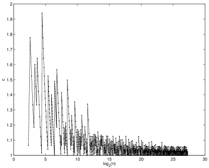
FIG. 2.: A plot of $c$ as a function of $n$, where $3cn$ is the number of intervals for an $n$-qubit scheme. The lower bound of $c$ is $1$. Using the Sylvester construction alone, $c$ fluctuates between $1$ and $2$ indefinitely.

In many applications, it may be useful to select more than one coupling term from the Hamiltonian. For example, one may select all coupling terms between the $i$-th and the $j$-th qubits in $H_{2}$, by choosing the $i$-th and the $j$-th rows of $S_{x,y,z}$ to be identical, and any other pairs of rows to be orthogonal. These $6$ identical rows have to be $++\cdots+$ in order to satisfy $S_{x}\mbox{.{\fds*}\hskip 0.43057pt}S_{y}=S_{z}$. The required number of intervals is the same as decoupling $n-2$ qubits. This pairwise coupling can further be changed to a desired form following methods in Refs. [10, 7]. Depending on circumstances, this composite method can reduce the operation time of the given Hamiltonian by a constant factor but can potentially increase the local resources by a constant factor. As a final remark, the selective coupling schemes in both Refs. [7, 11] are to first select the diagonal coupling terms or all coupling terms between a pair of qubits before further manipulations. The initial selection is done essentially using some version of the Sylvester construction, with even and arbitrary $r$ in Refs. [7] and [11] respectively.

V Universal Time reversal

We now apply the framework of sign matrices to simulate time reversal. As a first example, we apply the original framework in Ref. [2] to reverse $H_{1}$ given by Eq. (1). First construct a decoupling sign matrix $S_{n}$ for $n$ qubits using a normalized Hadamard matrix $H(\overline{n\!+\!1})$, excluding its first row. In this case, all entries in the first column of $S_{n}$ are “$+$”. A sign matrix for time reversal, denoted by $T_{n}$, is obtained by removing the first column of $S_{n}$. In $S_{n}$, any two rows have zero inner product, thus any two rows in $T_{n}$ have inner product $-1$, and any coupling term is reversed by exactly the same amount (note the significance of the $-$ sign in the inner product). Furthermore, each row of $S_{n}$ has zero row sum, so, each row in $T_{n}$ has row sum $-1$, and the local terms are reversed by the same amount as well. Therefore, any Hamiltonian given by Eq. (1) can be reversed. The simulation requires $n_{I}=\overline{n\!+\!1}-1$ intervals, and simulates the reversal for the duration of one interval. Hence the simulation factor [10] is $1/n_{I}$ or the overhead [8, 9] is $n_{I}$. The overhead is between $n$ and $n+3$ if Hadamard’s conjecture is true, and is $cn$ for $c\approx 1$ in any case. Without local terms, $n_{I}=\overline{n}-1$ ranges between $n-1$ and $n+2$ if Hadamard’s conjecture is true. Note that the protocol is independent of $H_{1}$, and can be applied to any $H_{1}$ which can even be unknown. We remark that a lower bound $n-1$ was derived for the much more specific and known Hamiltonian $H_{3}$ in Eq. (4) [9]. In view of this, the generality of the present result comes almost for “free”.

To reverse a Hamiltonian given by Eq. (2) using the generalized framework, we again construct sign matrices $S_{x,y,z}$ for a decoupling scheme (Section IV) with zero row sums. Furthermore, our constructions can be made to ensure all entries in the first columns of $S_{x,y,z}$ are $+$. Therefore, removing the first columns in $S_{x,y,z}$ results in a time reversal scheme. The overhead is again the number of intervals in the reversal scheme, which is $3cn$ for $c\approx 1$ for large $n$. Again, the same protocol applies to any $H_{2}$ and thus applies to unknown Hamiltonians as well.

As a comparison, the reversal method reported in Ref. [9] for $H_{4}$ given by Eq. (5) depends on the knowledge of $d_{\alpha}$, and whether they have the same sign or not. When all $d_{\alpha}$ have the same sign, the overhead is ${(n-1)|d_{x}+d_{y}+d_{z}|\over\max|d_{\alpha}|}$ or ${n|d_{x}+d_{y}+d_{z}|\over\max|d_{\alpha}|}$, which ranges from $\approx n-3n$. The generalized Hadamard matrix framework proposed can invert the much more general Hamiltonian in Eq. (2) with simulation factor only slightly larger than $3n$, without knowledge of the given Hamiltonian.

VI Conclusion

We have generalized the framework for Hamiltonian simulation and the methods for decoupling and selective coupling in Ref. [2]. We rederive, as a special case of our construction, the crucial step of selecting a coupling term in the simulation of $n$-qubit Hamiltonians in Ref. [7]. We also apply the technique to extend the time reversal problem considered in Ref. [9] from permutation invariant purely nonlocal Hamiltonians to an arbitrary $n$-qubit Hamiltonian.

Our framework based on sign matrices allows the complicated criteria for various simulation tasks to be rephrased in relatively simple orthogonality conditions, for which solutions can be obtained with the connections to Hadamard matrices.

VII Acknowledgments

This generalization was inspired by the work presented in Ref. [7]. We are indebted to Dominik Janzing, Marcus Stollsteimer, and Pawel Wocjan for pointing out a critical mistake in the initial version of the paper. The construction in Appendix B in the second version was partly inspired by the mention of OA(48,13,4,2) in Ref. [11]. We thank David DiVincenzo, Aram Harrow, and Barbara Terhal for helpful discussions and suggestions for the paper. We thank Robin Huang, Jim Leonard, and Kathleen Falcigno for providing the author with timely access to some important references. DWL is supported in part by the NSA and ARDA under the US Army Research Office, grant DAAG55-98-C-0041.

A Schur-subsets in Sylvester matrices

In this Appendix, we study the properties of the Sylvester matrices useful for decoupling, selective coupling or inversion of Hamiltonian. First of all, they are always normalized. We now describe a method to partition the rows of the Sylvester matrix $H(2)^{\otimes r}$ into $(2^{r}-1)/3$ and $(2^{r}-5)/3$ Schur-subsets when $r$ is even and odd respectively. It will be obvious from the construction that each $H(2)^{\otimes r}$ contains $5$ rows satisfying Eq. (62).

First, we introduce some notations. Let $\{0,1\}$ be the index set for the rows and columns of $H(2)=\left[\!\begin{array}[]{rr}1&\!\!\!1\\ 1&\!\!-1\end{array}\!\right]$. For example, the $(0,0)$ entry is $1$. We use the shorthand $H_{ij}$ for the $(i,j)$ entry of $H(2)$. Therefore $H_{ij}=(-1)^{ij}$. Likewise one can label the rows and columns of $H(2)^{\otimes r}$ with composite indices ${\bf i}=(i_{1},i_{2},\cdots,i_{r})$ which are $r$-bit strings. We have

$$H_{\bf ij} = H_{i_{1}j_{1}}\times H_{i_{2}j_{2}}\times\cdots\times H_{i_{r}j_{r}}$$ (A1)

$$= (-1)^{i_{1}j_{1}+i_{2}j_{2}+\cdots+i_{r}j_{r}}$$ (A2)

$$= (-1)^{{\bf i}\cdot{\bf j}}$$ (A3)

where ${\bf i}\cdot{\bf j}$ denotes the usual inner product of ${\bf i}$ and ${\bf j}$. For each ${\bf l}$,

$$H_{\bf il}\times H_{\bf jl}\times H_{\bf kl}=(-1)^{{\bf i}\cdot{\bf l}+{\bf j}\cdot{\bf l}+{\bf k}\cdot{\bf l}}=(-1)^{({\bf i}+{\bf j}+{\bf k})\cdot{\bf l}}\,.$$ (A4)

Therefore, the ${\bf i}$-th, ${\bf j}$-th, ${\bf k}$-th rows form a Schur-set iff $\forall_{\bf l}$ $H_{\bf il}\times H_{\bf jl}\times H_{\bf kl}=1$ iff ${\bf i}\oplus{\bf j}\oplus{\bf k}={\bf 0}$. We refer to such a triple of $r$-bit strings as a Schur-set also. The problem reduces to showing that, the set of non-zero $r$-bit strings partitions into $(2^{r}-1)/3$ and $(2^{r}-5)/3$ Schur-subsets when $r$ is even and odd respectively. This can be proved by separate inductions on the even and odd values of $r$.

For even values of $r\geq 2$, the induction hypothesis (IH) is that, the set of all $r$-bit strings partitions into $K=(2^{r}-1)/3$ Schur-subsets $E_{1}$, $E_{2}$, $\cdots$, $E_{K}$, and the singleton $\{{\bf 0}\}$. The IH is clearly true when $r=2$. Suppose it is true for some even $r\geq 2$. For each Schur-set $E_{i}=\{i_{1},i_{2},i_{3}\}$ of $r$-bit strings, we can obtain $4$ Schur-sets of $(r\!+\!2)$-bit strings:

$$\{01i_{1},10i_{2},11i_{3}\}$$ (A5)

$$\{01i_{2},10i_{3},11i_{1}\}$$ (A6)

$$\{01i_{3},10i_{1},11i_{2}\}$$ (A7)

$$\{00i_{1},00i_{2},00i_{3}\}$$ (A8)

We also have an addition Schur-set $\{01{\bf 0},10{\bf 0},11{\bf 0}\}$. Altogether, we find $4(2^{r}-1)/3+1=(2^{r+2}-1)/3$ Schur-sets of $(r\!+\!2)$-bit strings that include all strings except for $00{\bf 0}$. This completes the induction when $r$ is even. For odd values of $r\geq 3$, the IH is:

1. the set of all $r$-bit strings partitions into $K=(2^{r}-5)/3$ Schur-subsets $E_{1}$, $E_{2}$, $\cdots$, $E_{K}$, and a set of $5$ remainders $F=\{w_{1},w_{2},w_{3},w_{4},{\bf 0}\}$,

2. $E_{K}=\{k_{1},k_{2},k_{3}\}$ satisfies

   $$k_{1}=w_{1}\oplus w_{2}=w_{3}\oplus w_{4}\,,$$ (A9)

   $$k_{2}=w_{1}\oplus w_{3}=w_{2}\oplus w_{4}\,.$$ (A10)

For $r=3$, the IH is true, for example, by putting $E_{1=K}=\{001,100,101\}$, and $F=\{010,011,110,111,{\bf 0}\}$. Suppose the IH is true for some odd $r\geq 3$. Using the method of Eq. (A8), we obtain $4(K-1)$ Schur-subsets of $(r\!+\!2)$-bit strings from $E_{1}$, $\cdots$, $E_{K-1}$. There are $32$ remaining strings, $\{00,01,10,11\}\times\{k_{1},k_{2},k_{3},w_{1},w_{2},w_{3},w_{4},{\bf 0}\}$. If we represent distinct bit strings as distinct points, and Schur-sets as triangles, the IH implies the following relations for the $6$ $r$-bit strings:

(A11)

Note that two triangles that share a common vertice represent two Schur-sets that are not disjoint. From Eq. (A11), we can easily find another $8$ disjoint Schur-subsets of $(r\!+\!2)$-bit strings:

(A12)

Denote the remaining $8$ strings as $k^{\prime}_{1}=11{\bf 0}$, $k^{\prime}_{2}=01k_{3}$, $k^{\prime}_{3}=10k_{3}$, $w^{\prime}_{1}=00k_{3}$, $w^{\prime}_{2}=11k_{3}$, $w^{\prime}_{3}=01{\bf 0}$, $w^{\prime}_{4}=10{\bf 0}$, ${\bf 0^{\prime}}=00{\bf 0}$. An additional Schur-set $\{k^{\prime}_{1},k^{\prime}_{2},k^{\prime}_{3}\}$ can be formed, and the $5$ remaining rows $w^{\prime}_{i=,1,2,3,4},{\bf 0^{\prime}}$ cannot form any more Schur-set. Moreover, $k^{\prime}_{i},w^{\prime}_{i}$ satisfy Eq. (A10). Finally, the number of $(r\!+\!2)$-bit Schur-sets is $K^{\prime}=4((2^{r}-5)/3-1)+9=(2^{r+2}-5)/3$, completing the induction.

The inductive proof, together with the identification $H_{{\bf ij}}=(-1)^{{\bf i}\cdot{\bf j}}$, provides a constructive method to partition the rows of $H(2)^{\otimes r}$ into Schur-subsets.

Finally, the fact $H^{\otimes r}$ contains $5$ rows satisfying Eq. (62) is manifest for odd $r$ in Eq. (A10). In fact Eq. (62) is exactly equivalent to a pair of connected triangles as in Eq. (A11). The case for even $r$ follows by adding a “$0$” to each point in the joint triangles for odd $r$ in Eq. (A11).

B Construction using Generalized Hadamard matrices

In this Appendix, we construct Hadamard matrices of orders other than $2^{r}$ with the properties required of our schemes. This is done by composing a Hadamard matrix with a generalized Hadamard matrix [12].

Let $G$ be a group of order $g$, with group operation $\star$. A generalized Hadamard matrix over $G$ [12, 19], GH$(g,\lambda)$, is a $g\lambda\times g\lambda$ matrix whose entries $\gamma_{ij}$ are elements of $G$, and for $i\neq j$, the sequence $\{\gamma_{il}\star\gamma_{jl}^{-1}:1\leq l\leq g\lambda\}$ contains each element of $G$ $\lambda$ times. This sequence is the entry-wise “division” of the $i$-th row by the $j$-th row. For example, a Hadamard matrix $H(4n)$ is a GH$(2,2n)$ over the multiplicative group $\{+1,-1\}$.

We are interested in generalized Hadamard matrices over GF(4), with $g=4$ elements written in an unusual manner:

$$\left[\!\!\begin{array}[]{c}+\vspace*{-0.6ex}\\ +\vspace*{-0.6ex}\\ +\end{array}\!\!\right]\,,\left[\!\!\begin{array}[]{c}+\vspace*{-0.6ex}\\ -\vspace*{-0.6ex}\\ -\end{array}\!\!\right]\,,\left[\!\!\begin{array}[]{c}-\vspace*{-0.6ex}\\ +\vspace*{-0.6ex}\\ -\end{array}\!\!\right]\,,\left[\!\!\begin{array}[]{c}-\vspace*{-0.6ex}\\ -\vspace*{-0.6ex}\\ +\end{array}\!\!\right]\,.$$ (B1)

The group operation .*  is the entry-wise multiplication for the triples. The GH$(4,\lambda)$ is a $4\lambda\times 4\lambda$ array of triples (written as a column vector). For example, a possible GH$(4,1)$ is given by

$$\gamma=\left[\begin{array}[]{cccc}\left[\!\!\begin{array}[]{c}+\vspace*{-0.6ex}\\ +\vspace*{-0.6ex}\\ +\end{array}\!\!\right]&\left[\!\!\begin{array}[]{c}+\vspace*{-0.6ex}\\ +\vspace*{-0.6ex}\\ +\end{array}\!\!\right]&\left[\!\!\begin{array}[]{c}+\vspace*{-0.6ex}\\ +\vspace*{-0.6ex}\\ +\end{array}\!\!\right]&\left[\!\!\begin{array}[]{c}+\vspace*{-0.6ex}\\ +\vspace*{-0.6ex}\\ +\end{array}\!\!\right]\vspace*{1ex}\\ \left[\!\!\begin{array}[]{c}+\vspace*{-0.6ex}\\ +\vspace*{-0.6ex}\\ +\end{array}\!\!\right]&\left[\!\!\begin{array}[]{c}-\vspace*{-0.6ex}\\ -\vspace*{-0.6ex}\\ +\end{array}\!\!\right]&\left[\!\!\begin{array}[]{c}+\vspace*{-0.6ex}\\ -\vspace*{-0.6ex}\\ -\end{array}\!\!\right]&\left[\!\!\begin{array}[]{c}-\vspace*{-0.6ex}\\ +\vspace*{-0.6ex}\\ -\end{array}\!\!\right]\vspace*{1ex}\\ \left[\!\!\begin{array}[]{c}+\vspace*{-0.6ex}\\ +\vspace*{-0.6ex}\\ +\end{array}\!\!\right]&\left[\!\!\begin{array}[]{c}-\vspace*{-0.6ex}\\ +\vspace*{-0.6ex}\\ -\end{array}\!\!\right]&\left[\!\!\begin{array}[]{c}-\vspace*{-0.6ex}\\ -\vspace*{-0.6ex}\\ +\end{array}\!\!\right]&\left[\!\!\begin{array}[]{c}+\vspace*{-0.6ex}\\ -\vspace*{-0.6ex}\\ -\end{array}\!\!\right]\vspace*{1ex}\\ \left[\!\!\begin{array}[]{c}+\vspace*{-0.6ex}\\ +\vspace*{-0.6ex}\\ +\end{array}\!\!\right]&\left[\!\!\begin{array}[]{c}+\vspace*{-0.6ex}\\ -\vspace*{-0.6ex}\\ -\end{array}\!\!\right]&\left[\!\!\begin{array}[]{c}-\vspace*{-0.6ex}\\ +\vspace*{-0.6ex}\\ -\end{array}\!\!\right]&\left[\!\!\begin{array}[]{c}-\vspace*{-0.6ex}\\ -\vspace*{-0.6ex}\\ +\end{array}\!\!\right]\end{array}\right]$$ (B2)

We state some useful facts about generalized Hadamard matrices (see for example, Ref. [12] Part IV).

1. Equivalence [21]  Permuting rows or columns, or multiplying any row or column by a fixed element from the center of $G$ preserve the defining properties of a GH$(g,\lambda)$. Therefore, any GH$(g,\lambda)$ over an abelian group $G$ is equivalent to a normalized one, in which all entries in the first row and column are equal to the identity element in $G$.

2. Kronecker product [20, 21]  The Kronecker product of GH$(g,\lambda_{1})$ and GH$(g,\lambda_{2})$ over the same abelian group $G$ is a GH$(g,g\lambda_{1}\lambda_{2})$ over $G$.

3. [22] Let $q=g\lambda-1$ be a prime power. If GH$(g,\lambda)$ over $G$ exists, $\forall_{t\geq 0}$ GH$(g,\lambda q^{t})$ over $G$ exists.

Applying the above facts to GF(4), the existence of GH$(4,\lambda)$ for $\lambda=1,2$, implies that for $\lambda=1$, $2$, $3$, $4$, $8$, $9$, $12$, $14$, $16$, $24$, $27$, $33$, $\cdots$.

Let $H(m)$ be a Hadamard matrix with all the required properties: normalized, having $5$ rows $f_{i}$ satisfying Eq. (62), and having some $3n$ rows forming $n$ disjoint Schur-sets. We can assume that the rows of $H(m)$ are ordered so that members of each Schur-subset occur consecutively, starting from the first row, and the last $m-3n$ rows do not belong to any Schur-subsets. For example, the $1$-st to $3$-rd rows form a Schur-subset, and same for the $4$-th to $6$-th rows, and so on. Converting every $3$ consecutive rows into a row of triples. Do this for the first $3n$ rows of $H(m)$. The resulting array $\tilde{H}_{E}$ is an $n\times m$ array of triples. Call the last $m-3n$ rows of $H(m)$ $H_{F}$. For example,

$$H(2)^{\otimes 2} = \left[\begin{array}[]{cccc}+&-&+&-\\ +&+&-&-\\ +&-&-&+\\ +&+&+&+\end{array}\right]\,,$$ (B7)

$$\tilde{H}_{E} = \left[\begin{array}[]{cccc}\left[\!\!\begin{array}[]{c}+\vspace*{-0.6ex}\\ +\vspace*{-0.6ex}\\ +\end{array}\!\!\right]&\left[\!\!\begin{array}[]{c}-\vspace*{-0.6ex}\\ +\vspace*{-0.6ex}\\ -\end{array}\!\!\right]&\left[\!\!\begin{array}[]{c}+\vspace*{-0.6ex}\\ -\vspace*{-0.6ex}\\ -\end{array}\!\!\right]&\left[\!\!\begin{array}[]{c}-\vspace*{-0.6ex}\\ -\vspace*{-0.6ex}\\ +\end{array}\!\!\right]\end{array}\right]\,,$$ (B21)

$$H_{F} = \left[\begin{array}[]{cccc}+&+&+&+\end{array}\right]\,.$$ (B23)

As a second example, consider $H^{\otimes 4}$. The corresponding $H_{F}$ is $[+\cdots+]$. Following the previous Appendix, Schur-subsets of $4$-bit strings are $\{0101,1010,1111\}$ $\{0110,1011,1101\}$ $\{0111,1001,1110\}$ $\{0001,0010,0011\}$ $\{0100,1000,1100\}$. Thus, $\tilde{H}_{E}$ corresponding to $H(2)^{\otimes 4}$ is equal to

$$\left[\rule{0.0pt}{120.55518pt}\begin{array}[]{c|c|c|c|c|c|c|c|c|c|c|c|c|c|c|c}+&-&+&-&+&-&+&-&+&-&+&-&+&-&+&-\\ +&+&-&-&+&+&-&-&+&+&-&-&+&+&-&-\\ +&-&-&+&+&-&-&+&+&-&-&+&+&-&-&+\\ &&&&&&&&&&&&&&&\vspace*{-1.5ex}\hfil\\ \hline\cr&&&&&&&&&&&&&&&\vspace*{-1.5ex}\hfil\\ +&-&+&-&-&+&-&+&+&-&+&-&-&+&-&+\\ +&+&-&-&+&+&-&-&-&-&+&+&-&-&+&+\\ +&-&-&+&-&+&+&-&-&+&+&-&+&-&-&+\\ &&&&&&&&&&&&&&&\vspace*{-1.5ex}\hfil\\ \hline\cr&&&&&&&&&&&&&&&\vspace*{-1.5ex}\hfil\\ +&+&-&-&-&-&+&+&+&+&-&-&-&-&+&+\\ +&-&-&+&+&-&-&+&-&+&+&-&-&+&+&-\\ +&-&+&-&-&+&-&+&-&+&-&+&+&-&+&-\\ &&&&&&&&&&&&&&&\vspace*{-1.5ex}\hfil\\ \hline\cr&&&&&&&&&&&&&&&\vspace*{-1.5ex}\hfil\\ +&-&-&+&-&+&+&-&+&-&-&+&-&+&+&-\\ +&-&+&-&+&-&+&-&-&+&-&+&-&+&-&+\\ +&+&-&-&-&-&+&+&-&-&+&+&+&+&-&-\\ &&&&&&&&&&&&&&&\vspace*{-1.5ex}\hfil\\ \hline\cr&&&&&&&&&&&&&&&\vspace*{-1.5ex}\hfil\\ +&+&+&+&-&-&-&-&+&+&+&+&-&-&-&-\\ +&+&+&+&+&+&+&+&-&-&-&-&-&-&-&-\\ +&+&+&+&-&-&-&-&-&-&-&-&+&+&+&+\end{array}\right]$$ (B47)

Returning to the general construction, we now compose a normalized $\gamma=\mbox{GH}(g,\lambda)$ and $H(m)$ to form a new Hadamard matrix:

1. Take the Kronecker product $\tilde{H}_{E}\otimes\gamma$ (under .* ).

2. Convert each row of triples in $\tilde{H}_{E}\otimes\gamma$ back into $3$ rows of $\pm$ (an operation we call “leveling”). Call the resulting matrix $H^{\prime}_{E}$. It is $3n4\lambda\times m4\lambda$.

3. Take the first coordinates of each triple in $\gamma$ and form a $4\lambda\times 4\lambda$ matrix of entries $\pm$. Take the (usual) Kronecker product of $H_{F}$ with the above matrix to obtain $H^{\prime}_{F}$. It is $(m-3n)4\lambda\times m4\lambda$.

4. Append $H^{\prime}_{F}$ to $H^{\prime}_{E}$ to obtain an $m4\lambda\times m4\lambda$ matrix of $\pm 1$. Call this $H^{\prime}$.

We first show that the resulting matrix is indeed a Hadamard matrix. Denote by $\epsilon_{ij}$ the $(i,j)$ entry of the leveled $\gamma$, and $h_{ij}$ the $(i,j)$ entry of $H(m)$. Then, $H^{\prime}_{E}$ is explicitly given by:

$$\left[\begin{array}[]{c|c|c}\left[\!\!\begin{array}[]{c}h_{11}\vspace*{-0.6ex}\\ h_{21}\vspace*{-0.6ex}\\ h_{31}\end{array}\!\!\right]\mbox{.{\fds*}\hskip 0.43057pt}\left[\rule{0.0pt}{12.91663pt}~{}~{}\gamma~{}~{}\right]&\left[\!\!\begin{array}[]{c}h_{12}\vspace*{-0.6ex}\\ h_{22}\vspace*{-0.6ex}\\ h_{32}\end{array}\!\!\right]\mbox{.{\fds*}\hskip 0.43057pt}\left[\rule{0.0pt}{12.91663pt}~{}~{}\gamma~{}~{}\right]&~{}~{}\cdots{}{}\\ &&\vspace*{-1.5ex}\hfil\\ \hline\cr&&\vspace*{-1.5ex}\hfil\\ \left[\!\!\begin{array}[]{c}h_{41}\vspace*{-0.6ex}\\ h_{51}\vspace*{-0.6ex}\\ h_{61}\end{array}\!\!\right]\mbox{.{\fds*}\hskip 0.43057pt}\left[\rule{0.0pt}{12.91663pt}~{}~{}\gamma~{}~{}\right]&\left[\!\!\begin{array}[]{c}h_{42}\vspace*{-0.6ex}\\ h_{52}\vspace*{-0.6ex}\\ h_{62}\end{array}\!\!\right]\mbox{.{\fds*}\hskip 0.43057pt}\left[\rule{0.0pt}{12.91663pt}~{}~{}\gamma~{}~{}\right]&\\ &&\vspace*{-1.5ex}\hfil\\ \hline\cr&&\vspace*{-1.5ex}\hfil\\ \dots&\cdots&~{}~{}\cdots~{}~{}\rule{0.0pt}{12.91663pt}\end{array}\right]$$ (B67)

or

$$\left[\begin{array}[]{ccc|ccc|c}h_{11}\,\epsilon_{11}&h_{11}\,\epsilon_{12}&\cdots&h_{12}\,\epsilon_{11}&h_{12}\,\epsilon_{12}&\cdots{}&~{}~{}~{}\cdots{}{}{}\\ h_{21}\,\epsilon_{21}&h_{21}\,\epsilon_{22}&\cdots{}&h_{22}\,\epsilon_{21}&h_{22}\,\epsilon_{22}&\cdots{}&~{}~{}~{}\cdots{}{}{}\\ h_{31}\,\epsilon_{31}&h_{31}\,\epsilon_{32}&\cdots{}&h_{32}\,\epsilon_{31}&h_{32}\,\epsilon_{32}&\cdots{}&~{}~{}~{}\cdots{}{}{}\\ &&&&&&\vspace*{-1.5ex}\hfil\\ h_{11}\,\epsilon_{41}&h_{11}\,\epsilon_{42}&\cdots{}&h_{12}\,\epsilon_{41}&h_{12}\,\epsilon_{42}&\cdots{}&~{}~{}~{}\cdots{}{}{}\\ h_{21}\,\epsilon_{51}&h_{21}\,\epsilon_{52}&\cdots{}&h_{22}\,\epsilon_{51}&h_{22}\,\epsilon_{52}&\cdots{}&~{}~{}~{}\cdots{}{}{}\\ h_{31}\,\epsilon_{61}&h_{31}\,\epsilon_{62}&\cdots{}&h_{32}\,\epsilon_{61}&h_{32}\,\epsilon_{62}&\cdots{}&~{}~{}~{}\cdots{}{}{}\\ \vdots&\vdots&\ddots&\vdots&\vdots&\ddots&\\ &&&&&&\vspace*{-1.5ex}\hfil\\ \hline\cr&&&&&&\vspace*{-1.5ex}\hfil\\ h_{41}\,\epsilon_{11}&h_{41}\,\epsilon_{12}&\cdots{}&h_{42}\,\epsilon_{11}&h_{42}\,\epsilon_{12}&\cdots{}&~{}~{}~{}\cdots{}{}{}\\ h_{51}\,\epsilon_{21}&h_{51}\,\epsilon_{22}&\cdots{}&h_{52}\,\epsilon_{21}&h_{52}\,\epsilon_{22}&\cdots{}&~{}~{}~{}\cdots{}{}{}\\ h_{61}\,\epsilon_{31}&h_{61}\,\epsilon_{32}&\cdots{}&h_{62}\,\epsilon_{31}&h_{62}\,\epsilon_{32}&\cdots{}&~{}~{}~{}\cdots{}{}{}\\ &&&&&&\vspace*{-1.5ex}\hfil\\ h_{41}\,\epsilon_{41}&h_{41}\,\epsilon_{42}&\cdots{}&h_{42}\,\epsilon_{41}&h_{42}\,\epsilon_{42}&\cdots{}&~{}~{}~{}\cdots{}{}{}\\ h_{51}\,\epsilon_{51}&h_{51}\,\epsilon_{52}&\cdots{}&h_{52}\,\epsilon_{51}&h_{52}\,\epsilon_{52}&\cdots{}&~{}~{}~{}\cdots{}{}{}\\ h_{61}\,\epsilon_{61}&h_{61}\,\epsilon_{62}&\cdots{}&h_{62}\,\epsilon_{61}&h_{62}\,\epsilon_{62}&\cdots{}&~{}~{}~{}\cdots{}{}{}\\ \vdots&\vdots&\ddots&\vdots&\vdots&\ddots&\\ &&&&&&\vspace*{-1.5ex}\hfil\\ \hline\cr&&&&&&\\ \cdots&\cdots&\cdots&\cdots&\cdots&\cdots&\\ &&&&&&\end{array}\right]$$ (B90)

From Eq. (B90), the rows of $H^{\prime}_{E}$ are of the form:

$$[h_{i1},h_{i2},\cdots~{}]\otimes[\epsilon_{j1},\epsilon_{j2},\cdots~{}]$$ (B91)

where $i\in\{1,\cdots,3n\}$, $j\in\{1,\cdots,12\lambda\}$ and $i=j\bmod 3$. The rows of $H^{\prime}_{F}$ are of the same form, with $i\in\{3n\!+\!1,\cdots,m\}$, $j=3k+1$ for $k\in\{0,\cdots,4\lambda-1\}$. Thus each row in $H^{\prime}$ is specified by $i$ and $j$. Note that if $i\neq i^{\prime}$, $[h_{i1},h_{i2},\cdots~{}]$ and $[h_{i^{\prime}1},h_{i^{\prime}2},\cdots~{}]$ are orthogonal. If $j\neq j^{\prime}$ and $j=j^{\prime}\bmod 3$, then $[\epsilon_{j1},\epsilon_{j2},\cdots~{}]$ and $[\epsilon_{j^{\prime}1},\epsilon_{j^{\prime}2},\cdots~{}]$ are orthogonal since $\gamma$ is a generalized Hadamard matrix. Therefore, any two distinct rows in $H^{\prime}_{F}$ are orthogonal (orthogonal in at least one tensor component), and any row from $H^{\prime}_{E}$ is orthogonal to any row from $H^{\prime}_{F}$ (orthogonal in the first tensor component). Finally, let $i,j$ and $i^{\prime},j^{\prime}$ specify two distinct rows in $H^{\prime}_{E}$. If $i\neq i^{\prime}$, they are orthogonal in the first tensor component. If $i=i^{\prime}$, then $j\neq j^{\prime}$, $j=j^{\prime}\bmod 3$, and they are orthogonal in the second tensor component. Thus $H^{\prime}$ has orthogonal rows and is a Hadamard matrix.

Note that the rows of $H^{\prime}_{E}$ completely partition into Schur-subsets due to the group structure of the triples under .* . The ratio of the maximum number of qubits handled by the scheme to the number of intervals is the same in $H^{\prime}$ and $H(m)$ – everything is rescaled by a factor of $4\lambda$. This construction is therefore most useful when $H(m)$ has a large fraction of rows forming Schur-subsets, and when $\lambda$ is not a multiple of $4$.

One can verify that the above construction results in a normalized $H^{\prime}$ up to a permutation of the rows. Furthermore, because $\gamma$ is normalized $[h_{i1},h_{i2},\cdots~{}]\otimes[++\cdots~{}]$ occurs in $H^{\prime}$ for all $i$, Therefore, $H^{\prime}$ contains $5$ rows $f_{i}\otimes[++\cdots~{}]$ that satisfy Eq. (62).

Let the number of intervals required for an $n$-qubit scheme be $3cn$, and consider $c$ as a function of $n$. We now use the above construction to put a loose upper bound on $c$ for large $n$. A tighter bound on $c$ for smaller values of $n$ is plotted in Figure 2. A scheme formed by composing $H(m)=H(2)^{\otimes(r-2)}$ and $\gamma=\mbox{GH}(4,3^{(t+1)})$ has $2^{r}3^{(t+1)}$ intervals, and handles at least $(2^{r}-20)3^{\,t}$ qubits. For a given $n$, we find the smallest value of $(2^{r}-20)3^{\,t}$ larger than $n$. Let $n=2^{r_{o}+\Delta}$ where $\Delta\in[0,1)$, and $\epsilon=\log_{2}(2^{r}/(2^{r}-20))$. We look for the smallest non-negative value of

$$\log_{2}((2^{r}-20)3^{t}/n)=r-\epsilon+t\log_{2}3-r_{o}-\Delta$$ (B92)

where $t$, $r$ are positive integers. When $n$ is large, so is $r_{o}$. Since $\log_{2}3$ is irrational, $\{(t\log_{2}3)\bmod 1\}$ is a dense subset of $[0,1)$. We can find some $t\leq r_{o}/2\log_{2}3$ such that $t\log_{2}3=N+\delta$, $\delta\in[0,1)$, and $\delta-(\Delta+\epsilon\bmod 1)$ is small and nonnegative. We also choose $r=r_{o}-N+\lfloor\Delta+\epsilon\rfloor$. Note that $r$ is at least $r_{o}/2$. Then,

$$\log_{2}c = \log_{2}(2^{r}3^{t+1}/3n)$$ (B93)

$$= r+t\log_{2}3-r_{o}-\Delta$$ (B94)

$$= r_{o}-N+\lfloor\Delta+\epsilon\rfloor+N+\delta-r_{o}-\Delta$$ (B95)

$$= \lfloor\Delta+\epsilon\rfloor+\delta-\Delta-\epsilon+\epsilon$$ (B96)

$$= [\delta-(\Delta+\epsilon\bmod 1)]+\epsilon$$ (B97)

Both terms in the last line can be made small when $r_{o}$ is large, and $c\approx 1$.

REFERENCES

• [1] N. Linden, H. Barjat, R. Carbajo, and R. Freeman, Chem. Phys. Lett., 305:28–34, 1999, also arXive e-print quant-ph/9811043.
• [2] D.W. Leung, I.L. Chuang, F. Yamaguchi, and Y. Yamamoto, Phys. Rev. A, 61:042310, 2000, also arXive e-print quant-ph/9904100.
• [3] J. Jones and E. Knill, J. of Mag. Res., 141:322–5, 1999, also arXive e-print quant-ph/9905008.
• [4] D. DiVincenzo, Phys. Rev. A. 51, 1015, (1995).
• [5] A. Barenco, Proc. R. Soc. Lond. A (1995) 449, 679-83, also arXive e-print quant-ph/9505016, (1995).
• [6] D. Deutsch, A. Barenco and A. Ekert, Proc. R. Soc. Lond. A (1995) 449, 669-77, also arXive e-print quant-ph/9505018, (1995).
• [7] J.L. Dodd, M.A. Nielsen, M.J. Bremner, and R.T. Thew, arXive e-print quant-ph/0106064v1.
• [8] P. Wocjan, D. Janzing, and Th. Beth, arXive e-print quant-ph/0106077.
• [9] D. Janzing, P. Wocjan, and Th. Beth, arXive e-print quant-ph/0106085v1.
• [10] C.H. Bennett,  J.I. Cirac,  M.S. Leifer,  D.W. Leung, N. Linden, S. Popescu, G. Vidal, arXive e-print quant-ph/0107035.
• [11] M. Stollsteimer and G. Mahler, arXive e-print quant-ph/0107059v1.
• [12] C. Colbourn and J. Dinitz (Eds) The CRC Handbook of Combinatorial Designs (CRC Press, Boca Raton, 1996).
• [13] www.research.att.com/$\tilde{~{}}$njas/hadamard/index.html
• [14] J. van Lint and R. Wilson, A Course in Combinatorics (Cambridge University Press, Cambridge, 1992).
• [15] F. MacWilliams and N. Sloane, The Theory of Error-Correcting Codes (North Holland, Amsterdam, 1977).
• [16] J. Hadamard, Bull. Sciences Math., (2) 17 (1893), 240-246.
• [17] J. Sylvester, Phil. Mag. 34 (1867), 461-475.
• [18] R.E.A.C Paley, J. Math. Phys. 12 (1933), 311-320.
• [19] A.S. Hedayat, N.J.A. Sloane, and J. Stufken, Orthogonal Arrays, Theory and Applications (Springer Verlag, New York, 1999).
• [20] S.S. Shrikhandem, Canad., J. Math. 16 (1964), 131-141.
• [21] D.A. Drake, Canad. J. Math. 31 (1979), 617-627.
• [22] W. de Launey, Utilitas Math. 30 (1986), 5-29.