Perturbation Theory and Numerical Modeling
of Quantum Logic Operations
with a Large Number of Qubits

Abstract.

The perturbation theory is developed based on small parameters which naturally appear in solid state quantum computation. We report the simulations of the dynamics of quantum logic operations with a large number of qubits (up to 1000). A nuclear spin chain is considered in which selective excitations of spins are provided by having a uniform gradient of the external magnetic field. Quantum logic operations are utilized by applying resonant electromagnetic pulses. The spins interact with their nearest neighbors. We simulate the creation of the long-distance entanglement between remote qubits in the spin chain. Our method enables us to minimize unwanted non-resonant effects in a controlled way. The method we use cannot simulate complicated quantum logic (a quantum computer is required to do this), but it can be useful to test the experimental performance of simple quantum logic operations. We show that: (a) the probability distribution of unwanted states has a “band” structure, (b) the directions of spins in typical unwanted states are highly correlated, and (c) many of the unwanted states are high-energy states of a quantum computer (a spin chain). Our approach can be applied to simple quantum logic gates and fragments of quantum algorithms involving a large number of qubits.

Introduction

Recently much progress has been made in single particle technologies. These technologies allow one to manipulate a single electron, a single atom, and a single ion. A distinguishing feature of all these technologies is that they are “quantum”; quantum effects are crucial for the preparation of the initial state, for performing useful operations, and for reading out the final state. One of the future quantum technologies is quantum computation. In a quantum computer, the information is loaded in a register of quantum bits – “qubits”. A qubit is a quantum object (generalized spin 1/2) which can occupy two quantum states, $|0\rangle$ and $|1\rangle$, and an arbitrary superposition of these states: $\Psi=C_{0}|0\rangle+C_{1}|1\rangle$. (The only constraint is: $|C_{0}|^{2}+|C_{1}|^{2}=1$.) A quantum computer is remarkably efficient in executing newly invented quantum algorithms (the quantum Fourier transform, Shor’s algorithm for prime factorization, Grover’s algorithm for data base searching, and others). Using these algorithms, quantum computing promises to solve problems that are intractable on digital computers. The main advantage of quantum computation is the rapid, parallel execution of quantum logic operations. One of the promising directions in quantum computation is solid state quantum computation. (See the review [1].) In solid state computers, a qubit can be represented by a single nuclear spin 1/2 [2, 3], or a single electron spin 1/2 [4, 5], a single Cooper pair [6, 7]. This type of quantum computers is quite different from quantum computers in which a qubit is represented by an ensemble of spins 1/2 [8, 9, 10].

Crucial mathematical problems must be solved in order to understand the dynamical aspects of quantum computation. One of these problems is the creation of the dynamical theory of quantum computation – the main subject of our paper. The processes of the creation of quantum data bases, the storage and searching of quantum information, the implementation of quantum logic gates, and all the steps involved in quantum computation are dynamical processes. When qubits representing a register in a quantum computer are in superpositional states, they are not eigenstates of the Hamiltonian describing the quantum computer. These superpositions are time-dependent. Understanding their dynamics is very important. To design a working quantum computer, simulations of quantum logic operations and fragments of quantum computation are essential. The results of these simulations will enable engineers to optimize and test quantum computers.

There are two main obstacles to perform useful quantum logic operations with large number of qubits on a digital (classical) computer: (1) the related Hilbert space is extremely large, $D_{N}=2^{N}$, where $N$ is the number of qubits (spins), and (2) even if the initial state of a quantum computer does not involve many basic states (eigenstates), the number of excited eigenstates can rapidly grow during the process of performing quantum logic operations. Generally both of these obstacles exist. At the same time, many useful quantum operations can be simulated on a digital computer even if the number of qubits is quite large, say 1000. How one can do this? One way is to create (and use) a perturbation theory of quantum computation. To do this, one should consider a quantum computer as a many-particle quantum system and introduce small parameters. Usually, in all physical problems there exist small parameters which allow one to simplify the problem to find approximate solutions. The objective in this approach is to build a solution in a controlled way.

As an example, it is useful to consider an electron in a hydrogen atom interacting with a laser field. The electron has an infinite (formally) number of discrete levels plus a continuous part of its energy spectrum. So, a single electron in a Hydrogen atom has a Hilbert space larger than all finite qubit quantum computers. Assume that the electron is populated initially on some energy level(s). The action of the laser field on the electron leads in many cases to a regular and controlled dynamics of the electron. In particular, if the amplitude of the laser field is small enough, the electron interacting with this laser field can be considered as a two-level quantum system interacting with an external time-periodic field. Why is the electron excited to only few energy levels? This happens because the existence of small parameters makes the probability of unwanted events (excitation of the electron to most energy levels including the continuum) negligibly small. The existence of small parameters allows one to use perturbation approaches when calculating the quantum dynamics of the electron. This strategy can be used to create a perturbation theory of quantum computation.

In this paper we present our results, based on the existence of small parameters, for simulating quantum logic operations with a large number (up to 1000) of qubits. Our perturbation approach does not provide a substitution for computing quantum algorithms on a quantum computer. One will need quantum computer to do the required calculations. Our method will allow one to simulate the required benchmarks, quantum logic test operations, and fragments of quantum algorithms. Our method will enable engineers to optimize a working quantum computer.

In section 1, we formulate our model and the Hamiltonian of a quantum computer based on a one-dimensional nuclear spin chain. Spins interact through nearest-neighbor Ising interactions. All spins are placed in a magnetic field with the uniform gradient. This field gradient enables the selective excitation of spins. Quantum logic operations are provided by applying the required resonant electromagnetic pulses. In section 2, we present the dynamical equations of motion in the interaction representation. As well, we discuss an alternative description based on the transformation to the rotating frame. In the latter case the effective Hamiltonian is independent of time and solution of the problem can be obtained using the eigenstates of this Hamiltonian. In section 3, we derive simplified dynamical equations taking into account only resonant and near-resonant transitions (and neglecting non-resonant transitions). We introduce the small parameters which characterize the probability of generation of unwanted states in the result of near-resonant transitions. We describe a $2\pi k$-method which allows us to minimize the influence of unwanted near-resonant effects which can destroy quantum logic operations. In section 4, we describe a quantum Control-Not gate for remote qubits in a quantum computer with a large number of qubits. Analytical solution for this gate is presented in section 5, for the $2\pi k$ condition. In section 6, we present small parameters of the problem, in explicit form. The equation for the total probability of generation of unwanted states, including the states generated in the result of near-resonant and non-resonant transition, is derived in section 7. In section 8, we present results of numerical simulations of the quantum Control-Not gate for remote qubits in quantum computers with 200 and 1000 qubits when the probability of the near-resonant transitions is relatively large (when the conditions of $2\pi k$-method are not satisfied). We show that: (a) the probability distribution of unwanted states has a “band” structure, (b) the directions of spins in typical unwanted states are highly correlated, and (c) many of the unwanted states are high-energy states of the quantum computer (a spin chain). The total probability of error (including the states generated in the result of near-resonant and non-resonant transitions) is computed numerically in section 9 for small ($N=10$) and large ($N=1000$) number of qubits. A range of parameters is found in which the probability of error does not exceed a definite threshold. We test our perturbative approach using exact numerical solution when the number of qubits is small ($N=10$). In section 10, we show how the problem of quantum computation (even with large number of qubits) can be formulated classically in terms of interacting one-dimensional oscillators. In the conclusion, we summarize our results.

1. Formulation of the model

The mathematical model of a quantum computer used in this paper is based on a one-dimensional Ising nuclear-spin system – a chain of $N$ identical nuclear spins (qubits). Application of Ising spin systems for quantum computations was first suggested in Ref.[11]. Today, these systems are used in liquid nuclear magnetic resonance (NMR) quantum computation with small number of qubits [12]. The register (a 1D chain of $N$ identical nuclear spins) is placed in a magnetic field,

(1) $${\vec{B}}(t,\,z)=\left(b^{(n)}_{\perp}\cos\left[\nu^{(n)}t+\varphi^{(n)}\right],-b^{(n)}_{\perp}\sin\left[\nu^{(n)}t+\varphi^{(n)}\right],B^{z}(z)\right),$$

where $t^{(n)}\leq t\leq t^{(n+1)}$ and $n=1,...,M$. In (1), $B^{z}(z)$ is a slightly non-uniform magnetic field oriented in the positive $z$-direction. The quantities $b^{(n)}_{\perp}>0$, $\nu^{(n)}>0$ and $\varphi^{(n)}$ are, respectively, the amplitude, the frequency, and the initial phase of the circular polarized (in the $x-y$ plane) magnetic field. This magnetic field has the form of rectangular pulses of the length (time duration) $\tau^{(n)}=t^{(n+1)}-t^{(n)}$. The total number of pulses which is required to perform a given quantum computation (protocol) is $M$. Schematically, our quantum computer is shown in Fig. 1.

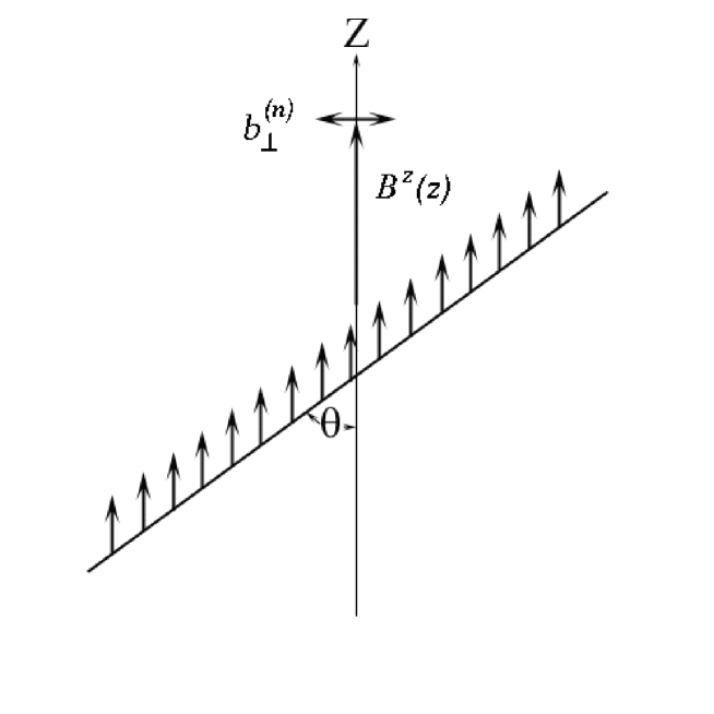
Figure 1. Nuclear spin quantum computer (the ground state of nuclear spins). $B^{z}(z)$ is the slightly non-uniform magnetic field; $b^{(n)}_{\perp}$ is the amplitude of radio-frequency field of the $n$-th rf pulse. The chain of spins makes an angle $\theta$ with the direction of the magnetic field $B^{z}(z)$.

1.1. The quantum computer Hamiltonian

The quantum Hamiltonian which describes our quantum computer has the form,

(2) $$\hat{H}=\hat{H}_{0}+\hat{V}=-\sum_{k=0}^{N-1}\omega_{k}\hat{I}^{z}_{k}-2J\sum_{k=0}^{N-2}\hat{I}^{z}_{k}\hat{I}^{z}_{k+1}+\hat{V}.$$

(We set $\hbar=1$.) The operator $\hat{V}$ describes the interaction of spins with pulses of the rf field,

(3) $$\hat{V}=\sum_{n=1}^{M}\hat{V}^{(n)},$$

and $\hat{V}^{(n)}$ describes the interaction of spins with $n$-th pulse of the rf field,

(4) $$\hat{V}^{(n)}=-\Theta^{(n)}(t){{\Omega^{(n)}}\over{2}}\sum_{k=0}^{N-1}\Bigg{\{}\hat{I}^{-}_{k}\exp\left[-i\left(\nu^{(n)}t+\varphi^{(n)}\right)\right]+$$

$$\hat{I}^{+}_{k}\exp\left[i\left(\nu^{(n)}t+\varphi^{(n)}\right)\right]\Bigg{\}},$$

where $\Theta^{(n)}(t)$ equals 1 only during the $n$th pulse. The operators in (2)-(4) have the following explicit form in the $z$-representation (the representation in which the operators $\hat{I}^{z}_{k}$ are diagonal),

(5) $$\hat{I}^{z}_{k}={{1}\over{2}}|0_{k}\rangle\langle 0_{k}|-{{1}\over{2}}|1_{k}\rangle\langle 1_{k}|,$$

$$\hat{I}^{+}_{k}=\hat{I}^{x}_{k}+i\hat{I}^{y}_{k}=|0_{k}\rangle\langle 1_{k}|,~{}\hat{I}^{-}_{k}=\hat{I}^{x}_{k}-i\hat{I}^{y}_{k}=|1_{k}\rangle\langle 0_{k}|.$$

We shall use the Dirac notation for the complete set of eigenstates (the stationary states) of the quantum computer described by the Hamiltonian $\hat{H}_{0}$ in (2). The eigenstates of the spin chain can be described as a combination of $2^{N}$ individual states of nuclear spins,

(6) $$|00...00\rangle,~{}|00...01\rangle,...,|11...11\rangle,$$

where the state $|0\rangle$ corresponds to the direction of a nuclear spin along the direction of the magnetic field, $B^{z}(z)$, and the state $|1\rangle$ corresponds to the opposite direction. The subscript “$k$” is omitted.

In (2)-(4), $\omega_{k}$ is the Larmor frequency of the $k$-th spin (neglecting interactions between spins), $\omega_{k}=\gamma B^{z}(z_{k})$, and $\gamma$ is the nuclear gyromagnetic ratio. (For example, for a proton in the field $B^{z}(z_{k})=10$T, one has the nuclear magnetic resonance (NMR) frequency $f_{k}=\omega_{k}/2\pi\approx 430$MHz.) We assume, for definiteness, that the gradient of the magnetic field is positive, $\partial B^{z}(z)/\partial z>0$. Suppose that the frequency difference of two neighboring spins is, $\delta f=\delta\omega/2\pi\approx 10$kHz, where $\delta\omega=\omega_{k+1}-\omega_{k}$. Thus, if the frequency of the edge spin is $430$MHz, the frequency of the spin at the other end of the chain of $1000$ qubits is $\approx 440$MHz. Then, the value of $B^{z}(z)$ increases by $\Delta B^{z}=0.23$T along the spin chain. Taking the distance between the neighboring spins, $a\approx 2\AA$, we obtain the characteristic value for the gradient of the magnetic field, $\partial B^{z}(z)/\partial z\approx 0.23/1000a\cos\theta$, where $\theta$ is the angle between the direction of the chain and the $z$-axis (Fig. 1). Below we will take $\cos\theta=1/\sqrt{3}$. (This allows one to suppress the dipole interaction between spins in the eigenstates of the Hamiltonian $\hat{H}_{0}$.) Thus, the gradient of the magnetic field is $\partial B^{z}(z)/\partial z\approx 2\times 10^{6}$T/m. The quantity $\Omega^{(n)}=\gamma b^{(n)}_{\perp}$ is the Rabi frequency of the $n$-th pulse.

2. Quantum dynamics of the computer

We discuss below the dynamics of the spin chain described by the Hamiltonian (2)-(4). The quantum state of the quantum computer is described by the wave function $\Psi(t)$. The dynamics of this function is given by the solution of the Schrödinger equation,

(7) $$i\dot{\Psi}(t)=\hat{H}\Psi(t),$$

where dot means derivative over time. This linear equation and an initial condition, $\Psi(0)$, define the state of the system at the time $t$. In this section we describe two different approaches which allow to solve Eq. (7).

2.1. Equations of motion in the interaction representation

In order to compute the dynamics it is convenient to go over to interaction representation. The wave function, $\Psi_{int}(t)$, in the interaction representation, is connected to the wave function, $\Psi(t)$, in the laboratory system of coordinates by the transformation,

(8) $$\Psi(t)=\hat{U}_{0}\Psi_{int}(t),~{}\hat{U}_{0}=\exp(-i\hat{H}_{0}t),$$

where, $\hat{H}_{0}$ is defined in (2). We choose the eigenfunctions, $|p\rangle$, and the eigenvalues, $E_{p}$, of the Hamiltonian $\hat{H}_{0}$ as the basis states and expand the wave function $\Psi_{int}(t)$ in a series,

(9) $$\Psi_{int}(t)=\sum_{p=0}^{2^{N}-1}C_{p}(t)|p\rangle,$$

where the states $|p\rangle$ satisfy the equation

(10) $$\hat{H}_{0}|p\rangle=E_{p}|p\rangle,~{}p=1,...,2^{N}.$$

The wave function in the laboratory system of coordinates has the form,

(11) $$\Psi(t)=\sum_{p}C_{p}(t)|p\rangle\exp(-iE_{p}t),$$

Using the Schrödinger equation (7) for the wave function, $\Psi(t)$, we obtain the equations of motion for the amplitudes $C_{p}(t)$,

(12) $$i\dot{C}_{p}=\sum_{m=0}^{2^{N}-1}C_{m}{V}^{(n)}_{pm}\exp\left[i(E_{p}-E_{m})t+ir_{pm}\left(\nu^{(n)}t+\varphi^{(n)}\right)\right],$$

which represent the wave function in the interaction representation. Here $r_{pm}=\mp 1$ for $E_{p}>E_{m}$ and $E_{p}<E_{m}$, respectively, ${V}^{(n)}_{pm}=-\Omega^{(n)}/2$ for the states $|p\rangle$ and $|m\rangle$ which are connected by a single-spin transition, and ${V}^{(n)}_{pm}=0$ for all other states.

2.2. The dynamics in the rotating frame

Sometimes, to calculate the quantum dynamics generated by the Hamiltonian (2) during the action of the $n$-th pulse, $t^{(n)}\leq t\leq t^{(n+1)}$, it is convenient to make a transformation to the system of coordinates which rotates with the frequency $\nu^{(n)}$ of the magnetic field, $\vec{b_{\perp}}$. To do this, one can use the unitary transformation [13],

(13) $$\hat{U}^{(n)}=\exp\Bigg{[}i\left(\nu^{(n)}t+\varphi^{(n)}\right)\sum_{k=0}^{N-1}\hat{I}^{z}_{k}\Bigg{]}.$$

In the rotating system of coordinates the new wave function, $\Psi_{rot}(t)$ and the new Hamiltonian, ${\mathcal{H}}^{(n)}$ have the form,

(14) $$\Psi_{rot}(t)=\hat{U}^{(n)+}\Psi(t),$$

(15) $$\hat{\mathcal{H}}^{(n)}=\hat{U}^{(n)+}\hat{H}^{(n)}\hat{U}^{(n)}=-\sum_{k=0}^{N-1}\Bigg{[}\left(\omega_{k}-\nu^{(n)}\right)\hat{I}^{z}_{k}+\Omega^{(n)}\hat{I}^{x}_{k}+2J\hat{I}^{z}_{k}\hat{I}^{z}_{k+1}\Bigg{]},$$

where the term $\hat{I}^{z}_{N-1}\hat{I}^{z}_{N}$ must be excluded. In the rotating system of coordinates the effective magnetic field which acts on the $k$-th spin during the action of the $n$-th pulse has the components,

(16) $$B^{(n)}_{k}=\left(\Omega^{(n)},0,\omega_{k}-\nu^{(n)}\right)/\gamma.$$

The advantage of the Hamiltonian (15) is that it is time-independent. In this case one can use the eigenstates of the Hamiltonian $\hat{\mathcal{H}}^{(n)}$ to calculate the dynamics during the $n$th pulse without solution of the system of differential equations (12). As before, we expand the wave function in the rotating frame, $\Psi_{rot}(t)$, over the eigenstates of the Hamiltonian $\hat{H}_{0}$,

(17) $$\Psi_{rot}(t)=\sum_{p=0}^{2^{N}-1}A_{p}(t)|p\rangle.$$

The wave function in the laboratory system of coordinates is,

(18) $$\Psi(t)=\sum_{p}A_{p}(t)|p\rangle\exp\left(-i\chi_{p}^{(n)}t+i\xi_{p}^{(n)}\right),$$

where $\chi_{p}^{(n)}=-\left(\nu^{(n)}/2\right)\sum_{k=0}^{2^{N}-1}\sigma_{k}^{p}$, $\xi_{p}^{(n)}=\left(\varphi^{(n)}/2\right)\sum_{k=0}^{2^{N}-1}\sigma_{k}^{p}$, $\sigma_{k}^{p}=-1$ if the state $|p\rangle$ contains the $k$th spin in in the state $|1\rangle$, and $\sigma_{k}^{p}=1$ if the state $|p\rangle$ contains the $k$th spin in the state $|0\rangle$. Below we take $\varphi^{(n)}=\xi_{p}^{(n)}=0$ for all $n$. The Schrödinger equation for the amplitudes $A_{p}(t)$, has the form,

(19) $$i\dot{A}_{p}(t)=\left(E_{p}-\chi_{p}^{(n)}\right)A_{p}(t)-\frac{\Omega^{(n)}}{2}\sum_{p^{\prime}}A_{p^{\prime}}(t),$$

where the sum is taken over the states $|p^{\prime}\rangle$ connected by a single-spin transition with the state $|p\rangle$.

Equation (19) can be written in the form $i\dot{A}_{p}(t)={\mathcal{H}}^{(n)}_{pp^{\prime}}A_{p^{\prime}}(t)$, where the effective Hamiltonian, $\hat{\mathcal{H}}^{(n)}$, is independent of time. When the number of spins, $N$, is not very large ($N<30$), one can diagonalize the Hamiltonian matrix ${\mathcal{H}}^{(n)}_{pp^{\prime}}$ and find its (time-independent) eigenfunctions,

(20) $$\psi^{(n)}_{q}=\sum_{p}A_{p}^{q\,(n)})|p\rangle$$

and eigenvalues, $e^{(n)}_{q}$. The amplitudes $A_{p}^{q\,(n)}$ are the eigenfunctions of the Hamiltonian $\hat{\mathcal{H}}^{(n)}$ in the representation of the Hamiltonian $\hat{H}_{0}$.

Using the eigenstates of the Hamiltonian $\hat{\mathcal{H}}^{(n)}$ one can calculate the dynamics generated by the $n$th pulse as,

(21) $$A_{p}(t_{n})=A_{p}=\sum_{p_{0}}A_{p_{0}}\sum_{q}A_{p_{0}}^{q\,(n)}A_{p}^{q\,(n)}\exp\left(-ie_{q}^{(n)}\tau_{n}\right),$$

where $t_{n}=t_{n-1}+\tau_{n}$, $\tau_{n}$ is the duration of the pulse, $A_{p_{0}}=A_{p}(t_{n-1})$ is the amplitude before the action of the $n$th pulse, $A_{p}=A_{p}(t_{n})$ is the amplitude after the action of the $n$th pulse.

The amplitudes, $A_{p}(t)$, in the rotating frame are related to the amplitudes, $C_{p}(t)$, in the interaction representation by (see Eqs. (11) and (18)),

(22) $$A_{p}(t)=\exp(-i{\mathcal{E}}_{p}^{(n)}t)C_{p}(t),$$

Where ${\mathcal{E}}_{p}^{(n)}=E_{p}-\chi_{p}^{(n)}$ are the diagonal elements of the Hamiltonian matrix ${\mathcal{H}}_{pp^{\prime}}^{(n)}$. Since the rf pulses in the protocol are different, the effective time-independent Hamiltonians, ${\mathcal{H}}_{pp^{\prime}}^{(n)}$, are also different for different $n$. Hence, before each $n$th pulse we should make the transformation to the rotating frame, $C_{p}(t_{n-1})\rightarrow A_{p}(t_{n-1})$, and after the pulse we must return to the interaction representation $A_{p}(t_{n})\rightarrow C_{p}(t_{n})$.

In the rotating frame the most difficult problem is the diagonalization of the sparse symmetric matrices (for each pulse) of the size $2^{N}\otimes 2^{N}$. (In each row of this matrix there are only $N+1$ nonzero matrix elements.) This approach can be used directly (without perturbative consideration) only for small quantum computers, with the number of qubits $N<30$. For our purposes, to model quantum dynamics in a quantum computer with large number of qubits ($N=1000$), we shall use a perturbation approach based on the existence of small parameters.

3. Resonant and near-resonant transitions

The number of equations in (12) grows exponentially as $N$ increases. Thus, this system of equations cannot be solved directly when $N$ is large. Our intention is to solve Eqs. (12) or (19) approximately, but in a controlled way. This can be done if we make use of small parameters which exist for the system. The explicit expressions for small parameters will be given below, in sections 8 and 9.

3.1. Resonant and non-resonant frequencies

In this section, we describe the main simplification procedure which is based on the separation of resonant and non-resonant interactions. This procedure is commonly used in studying linear and non-linear dynamical systems [14, 15, 16]. The main idea of this approach is the following. When the frequency of the external field, $\nu^{(n)}$, is equal (or close) to the eigenfrequency of the system under consideration, $\omega_{pm}\equiv E_{p}-E_{m}$, and when a small parameter exists (the interaction is relatively weak), one can separate the slow (resonant) dynamics from the fast (non-resonant) dynamics. The main contribution to the evolution of the system is associated with resonant effects. Usually, non-resonant effects are small, and can be considered using perturbation approaches. In quantum computation, the problem of non-resonant effects is more complicated because these effects can accumulate in time creating significant errors in the process of quantum computation. So, in quantum computation, the non-resonant effects must not only be taken into consideration, but they must also be minimized. Below, we describe methods which allow us to minimize the influence of non-resonant effects.

In classical dynamical systems, the separation of resonant and non-resonant effects is very efficient when “action-angle” variables are used. In this case, the “action” is a slow variable and the “angle” (the “phase”) is a fast variable. From this point of view, Eqs. (12) are convenient because they are written in the “energy” representation in which the slow (resonant) effects and fast (non-resonant) effects can be naturally separated.

First, we note that as the number of spins, $N$, increases, the number of eigenstates, $|p\rangle$, increases exponentially (as $2^{N}$), but the number of resonant frequencies in our system grows only linearly in $N$. Indeed, the number of resonant frequencies is $3N-2$ because only single-spin transitions are allowed by the operator $\hat{V}$ in (3). The definition of the resonant frequency is the following. We introduce the frequency of the single-spin transition: $\omega_{pm}\equiv E_{p}-E_{m}$, where $E_{p}$ and $E_{m}$ are two eigenstates, $|p\rangle$ and $|m\rangle$, of the Hamiltonian $\hat{H}_{0}$ with opposite orientations of only the $k$-th spin, ($k=0,...,N-1$). For example,

(23) $$|p\rangle=|n_{N-1}n_{N-2}...0_{k}...n_{1}n_{0}\rangle,~{}|m\rangle=|n_{N-1}n_{N-2}...1_{k}...n_{1}n_{0}\rangle,$$

where $n_{k}=0,1$. The resonant frequency for transition between $p$th and $m$th states, $\nu^{(n)}_{res}$, of the $n$-th external rf pulse is defined as follows:

(24) $$\nu^{(n)}_{res}=|\omega_{pm}|.$$

The only resonant frequencies of our nuclear spin quantum computer are,

(25) $$~{}~{}~{}\,\qquad\omega_{k}\pm J,\qquad\qquad\,\,(k=0,~{}or~{}k=N-1),$$

$$\omega_{k},~{}\omega_{k}\pm 2J,\qquad(1\leq k\leq N-2),$$

where the Larmor frequencies, $\omega_{k}=\gamma B^{z}(z_{k})$. All resonant frequencies in (25) are assumed to be positive. For end spins with $k=0$ and $k=N-1$, the upper and lower signs in (25) correspond to the states $|0\rangle$ or $|1\rangle$ of their only neighboring spins. For inner spins with $1\leq k\leq N-2$ the frequency $\omega_{k}$ corresponds to having nearest neighbors whose spins are in opposite directions to each other. The “+” sign corresponds to having the nearest neighbors in their ground state. The “-” sign corresponds to having the nearest neighbors in their excited state.

As an example, consider the resonant frequency of a single-spin transition between the following two eigenstates,

$$|p\rangle=|n_{N-1}n_{N-2}...1_{k-1}0_{k}1_{k+1}...n_{1}n_{0}\rangle,$$

$$|m\rangle=|n_{N-1}n_{N-2}...1_{k-1}1_{k}1_{k+1}...n_{1}n_{0}\rangle.$$

These two eigenstates differ by a transition of the $k$-th spin from its ground state, $|0_{k}\rangle$, to its excited state, $|1_{k}\rangle$. All other spins in the quantum computer remain in their initial states. According to (2), the eigenvalues of the states $|p\rangle$ and $|m\rangle$ are:

(26) $$E_{p}=E_{nres}-{{\omega_{k}}\over{2}}+J,\qquad E_{m}=E_{nres}+{{\omega_{k}}\over{2}}-J,$$

where $E_{nres}$ is the total energy of all $N-1$ (except the $k$-th) which did not participate in the transition. It follows from (26) that in this case, the resonance frequency, $\nu^{(n)}_{res}$, of the $n$-th pulse is,

(27) $$\nu^{(n)}_{res}=|E_{p}-E_{m}|=\omega_{k}-2J.$$

This frequency belongs to the set of the resonant frequencies introduced in (25). In the following, we assume that our protocol includes only the resonant frequencies from (18), and we will omit the subscript “res”.

3.2. Dynamical equations for resonant and near-resonant transitions

In this sub-section we derive the approximate equations for resonant and near-resonant transitions, in the system. Consider an arbitrary eigenstate of the Hamiltonian $\hat{H}_{0}$,

(28) $$|n_{N-1}n_{N-2}...n_{1}n_{0}\rangle,$$

where, as before, the subscript indicates the position of the spin in a chain, and $n_{k}=0,1$. Assume that one applies to the spin chain a resonant rf pulse of a frequency, $\nu^{(n)}$, from (25). Then, one has two possibilities:
1) The frequency of the pulse, $\nu^{(n)}$, is the resonant frequency of the state (28).
2) The frequency, $\nu^{(n)}$, differs from the closest resonant frequency of the state (28) by the value $\Delta=\pm 2J$ or $\pm 4J$ (near-resonant frequency).

In the first case, one has a resonant transition. In the second case, one has a near-resonant transition. If the small parameters exist, $J/\delta\omega\ll 1$, and $\Omega/\delta\omega\ll 1$, we can neglect all non-resonant transitions related to a flip of $k^{\prime}$th non-resonant spin. Below, in section 9, we will write a rigorous condition for $\delta\omega$ which is required in order to neglect all non-resonant transitions.

Thus, considering the dynamics of any state (28) under the action of an rf pulse with the frequency, $\nu^{(n)}$, from (24), (25), we need only to take into account one transition. This transition will be either a resonant one or a near-resonant one. This allows us to reduce the system of equations (12) to the set of only two coupled equations (two-level approximation),

(29) $$~{}~{}~{}~{}~{}~{}i\dot{C}_{p}=-(\Omega^{(n)}/2)\exp[i(E_{p}-E_{m}-\nu^{(n)})t]C_{m},$$

$$i\dot{C}_{m}=-(\Omega^{(n)}/2)\exp[i(E_{m}-E_{p}+\nu^{(n)})t]C_{p},$$

where $E_{p}>E_{m}$, $|p\rangle$ and $|m\rangle$ are any two eigenstates which are connected by a single-spin transition and whose energies differ by $\nu^{(n)}$ or $\nu^{(n)}+\Delta_{pm}^{(n)}$, where $\Delta_{pm}^{(n)}=E_{p}-E_{m}-\nu^{(n)}$ is the frequency detuning for the transition between the states $|p\rangle$ and $|m\rangle$.

3.3. Solutions of the dynamical equations in two-level approximation

The solution of Eqs. (29) for the case when the system is initially in the eigenstate $|m\rangle$, is,

(30) $$C_{m}(t_{0}+\tau)=\left[\cos(\lambda_{pm}\tau/2)+i(\Delta_{pm}/\lambda_{pm})\sin(\lambda_{pm}\tau/2)\right]\times\exp(-i\tau\Delta_{pm}/2),$$

$$C_{p}(t_{0}+\tau)=i(\Omega/\lambda_{pm})\sin(\lambda_{pm}\tau/2)\times\exp(it_{0}\Delta_{pm}+i\tau\Delta_{pm}/2),$$

$$C_{m}(t_{0})=1,\qquad C_{p}(t_{0})=0,$$

where $\lambda_{pm}=(\Omega^{2}+\Delta_{pm}^{2})^{1/2}$, $t_{0}$ is the time of the beginning of the pulse; $\tau$ is the duration of the pulse. Here and below we omit the upper index “$(n)$” which indicates the number of the rf pulse. If the system is initially in the upper state, $|p\rangle$, ($C_{m}(t_{0})=0$, $C_{p}(t_{0})=1$), the solution of (29) is,

(31) $$C_{p}(t_{0}+\tau)=[\cos(\lambda_{pm}\tau/2)-i(\Delta_{pm}/\lambda_{pm})\sin(\lambda_{pm}\tau/2)]\times\exp(i\tau\Delta_{pm}/2),$$

$$C_{m}(t_{0}+\tau)=i(\Omega/\lambda_{pm})\sin(\lambda_{pm}\tau/2)\times\exp(-it_{0}\Delta_{pm}-i\tau\Delta_{pm}/2),$$

$$C_{p}(t_{0})=1,\qquad C_{m}(t_{0})=0.$$

For the resonant transition ($\Delta_{pm}=0$), the expressions (30) and (31) transform into the well-known equations for the Rabi transitions. For example, we have from (30) for $\Delta_{pm}=0$,

$$C_{m}(t_{0}+\tau)=\cos(\Omega\tau/2),\qquad C_{p}(t_{0}+\tau)=i\sin(\Omega\tau/2).$$

In particular, for $\Omega\tau=\pi$ (the so-called $\pi$-pulse), the above expressions describe the complete transition from the state $|m\rangle$ to the state $|p\rangle$.

For the near-resonant transitions, consider two characteristic parameters in expressions (30) and (31):

$$\epsilon^{(1)}_{pm}=\Omega/\lambda_{pm},\qquad\epsilon^{(2)}_{pm}=\sin(\lambda_{pm}\tau/2).$$

If either of these two parameters, $\epsilon^{(1)}_{pm}$ or $\epsilon^{(2)}_{pm}$, is zero, the probability of a non-resonant transition vanishes. The second parameter, $\epsilon^{(2)}_{pm}$, is equal zero when,

(32) $$\lambda_{pm}\tau=2\pi k,\qquad(k=1,2,..),$$

where $k$ is the number of revolutions of the non-resonant (average) spin about the effective field in the rotating frame. Eq. (32) is the condition for the “$2\pi k$”-method to eliminate the near-resonant transitions. (See [13], Chapter 22, and [17, 18].)

3.4. The $2\pi k$-method

We shall present here the explicit conditions for the “$2\pi k$” rotation from the state $|p\rangle$ to the state $|m\rangle$. For a $\pi$-pulse ($\Omega\tau=\pi$), the values of $\Omega$ which satisfy the $2\pi k$ condition are, according to Eq. (32),

(33) $$\Omega^{[k]}_{pm}=|\Delta_{pm}|/\sqrt{4k^{2}-1}=|\Delta_{pm}|/\sqrt{3},~{}|\Delta_{pm}|/\sqrt{15},~{}|\Delta_{pm}|/\sqrt{35},~{}|\Delta_{pm}|/\sqrt{63},...$$

For a $\pi/2$-pulse, the corresponding values of $\Omega$ are,

(34) $$\Omega^{[2k]}_{pm}=|\Delta_{pm}|/\sqrt{16k^{2}-1}=|\Delta_{pm}|/\sqrt{15},~{}|\Delta_{pm}|/\sqrt{63},\dots$$

(If the Rabi frequency, $\Omega$, satisfies the $2\pi k$ condition (34) for a $\pi/2$-pulse, it automatically satisfies the condition (33) for a $\pi$-pulse.)

3.5. Resonant and near-resonant transitions in the rotating frame

We consider here the structure of the effective time-independent Hamiltonian matrix ${\mathcal{H}}_{pp^{\prime}}$ in the rotating frame. We discuss the two-level approximation in the rotating system of coordinates and demonstrate equivalence of the solution in the rotating frame with the solution (30) (or (31)) in the interaction representation.

Let us discuss the structure of the matrix ${\mathcal{H}}_{pp^{\prime}}$. Since the spins in the chain are identical, all nonzero non-diagonal matrix elements are the same and equal to ($-\Omega/2$). At $\Omega\ll\delta\omega$ the absolute values of the diagonal elements in general case are much larger than the absolute values of the off-diagonal elements. We explain below how the resonance is coded in the structure of the diagonal elements of the Hamiltonian matrix, ${\mathcal{H}}_{pp^{\prime}}$.

Suppose that the $k$th spin in the chain has resonant or near-resonant NMR frequency. The energy separation between $p$th and $m$th diagonal elements of the matrix ${\mathcal{H}}_{pp^{\prime}}$ related by the flip of resonant (or near-resonant) $k$th spin is much less than the energy separation between the $p$th diagonal elements and diagonal elements related to other states, which differ from the state $|p\rangle$ by a flip of a non-resonant $k^{\prime}$th ($k^{\prime}\neq k$) spin. In this case one can neglect the interaction of the $p$th state with all states except for the state $|m\rangle$, and the Hamiltonian matrix ${\mathcal{H}}_{pp^{\prime}}$ breaks up into $2^{N}/2$, approximately independent $2\times 2$ matrices,

(35) $$\begin{pmatrix}{\mathcal{E}}_{m}&V\\ V&{\mathcal{E}}_{p},\end{pmatrix}$$

where $E_{p}=E_{m}+\Delta_{pm}$, $|\Delta_{pm}|\sim J$ or zero, and $V=-\Omega/2$ is the perturbation amplitude.

Suppose, for example, that $N=5$ and third spin ($k=3$) has resonant or near-resonant frequency. (We start enumeration from the right as shown in (23).) Then, the block $2\times 2$ will be organized, for example, by the following states: $|01010\rangle$ and $|00010\rangle$; $|01111\rangle$ and $|00111\rangle$; $|00001\rangle$ and $|01001\rangle$, and so on. In order to find the state $|m\rangle$, which form $2\times 2$ block with a definite state $|p\rangle$, one should flip the resonant spin of the state $|p\rangle$. In other words, positions of $N-1$ (non-resonant) spins of these states are equivalent, while position of the resonant spin is different.

We now obtain the solution in the two-level approximation. The dynamics is given by Eq. (21). Since we deal only with a single $2\times 2$ block of the matrix ${\mathcal{H}}_{pp^{\prime}}$, (but not with the whole matrix), the dynamics in this approximation is generated only by the eigenstates of one block. In order to demonstrate equivalence of two descriptions (in the rotating frame and in the interaction representation) we will choose the same initial condition as in (30). Then, we will make the transformation (22) to the rotating frame, $C_{p}\rightarrow A_{p}$. After that we shall compute the dynamics by Eq. (21) and return to the interaction representation, $A_{p}\rightarrow C_{p}$, using Eq. (22). Eventually, we will obtain Eq. (30). The result is the same in the rotating frame and in the interaction representation. Physically these two approaches are equivalent (exactly, but not only in the two-level approximation), but mathematically they are different. In the interaction representation we calculate the dynamics generated by the time-dependent Hamiltonian. There are no stationary states in this case and one should solve the system of differential equations. On the other hand, in the rotating frame the effective Hamiltonian $\hat{\mathcal{H}}$ is time-independent and the wave function evolves in time because it is not the eigenfunction of $\hat{\mathcal{H}}$.

The eigenvalues $e^{(0)}_{q}$, $e^{(0)}_{Q}$, and the eigenfunctions of the $2\times 2$ matrix (35) are (we put $\Delta_{pm}=\Delta$ and $\lambda_{pm}=\lambda$),

(36) $$e^{(0)}_{q}={\mathcal{E}}_{m}+\frac{\Delta}{2}-\frac{\lambda}{2},\qquad\begin{pmatrix}A^{q\,(0)}_{m}\\ A^{q\,(0)}_{p}\end{pmatrix}={1\over\sqrt{(\lambda-\Delta)^{2}+\Omega^{2}}}\begin{pmatrix}\Omega\\ \lambda-\Delta\end{pmatrix},$$

(37) $$e^{(0)}_{Q}={\mathcal{E}}_{m}+\frac{\Delta}{2}+\frac{\lambda}{2},\qquad\begin{pmatrix}A^{Q\,(0)}_{m}\\ A^{Q\,(0)}_{p}\end{pmatrix}={1\over\sqrt{(\lambda-\Delta)^{2}+\Omega^{2}}}\begin{pmatrix}-(\lambda-\Delta)\\ \Omega\end{pmatrix}.$$

Suppose that before the $n$th pulse the system is in the state $|m\rangle$, i.e. the conditions

$$C_{m}(t_{0})=1,\qquad C_{p}(t_{0})=0,$$

are satisfied. After the transformation, (22), to the rotating frame we obtain

$$A_{m}(t_{0})=\exp(-i{\mathcal{E}}_{m}t_{0})C_{m}(t_{0})=\exp(-i{\mathcal{E}}_{m}t_{0}),\qquad A_{p}(t_{0})=0.$$

The dynamics is given by Eq. (21), which in our case takes the form:

$$A_{m}(t)=A_{m}(t_{0})\left[\left(A_{m}^{q\,(0)}\right)^{2}\exp\left(-ie^{(0)}_{q}\tau\right)+\left(A_{m}^{Q\,(0)}\right)^{2}\exp\left(-ie^{(0)}_{Q}\tau\right)\right]=$$

$${\exp\left[-i[{\mathcal{E}}_{m}t-(\Delta/2)\tau]\right]\over\Omega^{2}+(\lambda-\Delta)^{2}}\left\{\Omega^{2}e^{-i\lambda\tau/2}+(\lambda-\Delta)^{2}e^{i\lambda\tau/2}\right\},$$

where $t=t_{0}+\tau$. Applying the back transformation,

$$C_{m}(t)=\exp(i{\mathcal{E}}_{m}t)A_{m}(t),$$

and taking the real and imaginary parts of the expression in curl brackets we obtain the first equation (30). For another amplitude we have,

$$A_{p}(t)=A_{m}(t_{0})\left[A_{m}^{q\,(0)}A_{p}^{q\,(0)}\exp\left(-ie^{(0)}_{q}\tau\right)+A_{m}^{Q\,(0)}A_{p}^{Q\,(0)}\exp\left(-ie^{(0)}_{Q}\tau\right)\right]=$$

$$i{\Omega\over\lambda}\exp\left\{-i\left[{\mathcal{E}}_{m}t-(\Delta/2)\tau\right]\right\}\sin(\lambda\tau/2).$$

Applying the back transformation,

$$C_{p}(t)=\exp[i({\mathcal{E}}_{m}+\Delta)t]A_{p}(t),$$

we obtain the second equation in (30).

One may demonstrate the equivalence of our two approaches in a different, more simple, way. The dynamical equations with the $2\times 2$ Hamiltonian (35) are,

$$i\dot{A}_{p}={\mathcal{E}}_{p}A_{p}+VA_{m},$$

$$i\dot{A}_{m}=VA_{p}+{\mathcal{E}}_{m}A_{m}.$$

After the transformation (22) to the interaction representation we obtain,

(38) $$~{}~{}~{}~{}~{}i\dot{C}_{p}=V\exp[i({\mathcal{E}}_{p}-{\mathcal{E}}_{m})t]C_{m},$$

$$i\dot{C}_{m}=V\exp[i({\mathcal{E}}_{m}-{\mathcal{E}}_{p})t]C_{p},$$

where ${\mathcal{E}}_{p}-{\mathcal{E}}_{m}=E_{p}-E_{m}-\nu=\Delta_{pm}$, $V=-\Omega/2$. One can see that Eqs. (38) are equivalent to Eqs. (29) with the solution given by (30) or (31).

4. A quantum Control-Not gate for remote qubits

The quantum Control-Not ($CN_{kl}$) gate is a unitary operator which transforms the eigenstate,

(39) $$|n_{N-1}...n_{k}.......n_{l}....n_{0}\rangle,$$

into the state,

(40) $$|n_{N-1}...n_{k}.......\bar{n}_{l}....n_{0}\rangle,$$

where $\bar{n}_{l}=1-n_{l}$ if $n_{k}=1$; and $\bar{n}_{l}=n_{l}$ if $n_{k}=0$. The $k$-th and $l$-th qubits are called the control and the target qubits of the $CN_{kl}$ gate. One can also introduce a modified quantum $CN$ gate which performs the same transformation (39), (40) accompanied by phase shifts which are different for different eigenstates [13]. It is well-known that the quantum $CN$ gate can produce an entangled state of two qubits, which cannot be represented as a product of the wave functions of the individual qubits.

In this section, we shall consider an implementation of the quantum $CN$ gate in the Ising spin chain with the left end spin as the control qubit and the right end spin as the target qubit, i.e. $CN_{N-1,0}$ for a spin chain with large number of qubits, $N$ ($N=200$ or $N=1000$). Using this quantum gate we will create entanglement between the end qubits in the spin chain.

Assume that initially a quantum computer is in its ground state,

(41) $$\Psi=|0...0\rangle.$$

Then we apply a $\pi/2$-pulse with the resonant frequency,

(42) $$\nu=\omega_{N-1}.$$

The $\pi/2$-pulse means that the duration of this pulse is $\tau=\pi/2\Omega$. This pulse produces a superpositional state of the $(N-1)$-th (left) qubit,

(43) $$\Psi=(1/\sqrt{2})(|0...0\rangle+i|1...0\rangle).$$

To implement a modified quantum $CN_{N-1,0}$ gate we apply to the spin chain $M=2N-3$ $\pi$-pulses which transform the state $|10\dots 00\rangle$ to the state $|10\dots 01\rangle$ by the following scheme: $|1000\dots 0\rangle\rightarrow|1100\dots 0\rangle\rightarrow|1110\dots 0\rangle\rightarrow$ $|1010\dots 0\rangle\rightarrow|1011\dots 0\rangle\rightarrow|1001\dots 0\rangle\rightarrow$ $\dots\rightarrow|100\dots 11\rangle\rightarrow|100\dots 01\rangle.$ All frequencies of our protocol are resonant for these transitions. If we apply the same protocol to the system in the ground state, then with large probability the system will remain in the ground state because these pulses have the detunings from resonant transitions, $\Delta_{n}=\Delta^{(n)}_{0m}\neq 0$. Here the ground state $|0\rangle=|00\dots 00\rangle$ is related to the state $|m\rangle$ by the flip of the $k$th spin with the near-resonant NMR frequency. The first $\pi$-pulse has the frequency $\omega=\omega_{N-2}$. For the second $\pi$-pulse $\omega=\omega_{N-3}$. For the third $\pi$-pulse, $\omega=\omega_{N-2}-2J$, etc. All detunings, $\Delta_{n}$, in our protocol are the same, $\Delta_{n}=2J$, except for the third pulse, where $\Delta_{3}=4J$.

5. An analytic solution with application of a $2\pi k$-method

Assume that all $M$ $\pi$-pulses satisfy the $2\pi k$ condition, with the same value of $k$:

(44) $$\lambda_{n}^{[k]}\tau_{n}=2\pi k,({\rm and}~{}\Omega_{n}^{[k]}\tau_{n}=\pi),$$

where $\lambda^{[k]}_{n}=\sqrt{\left(\Omega^{[k]}_{n}\right)^{2}+\Delta_{n}^{2}}$. In this case, we can derive an analytic expression for the wave function, $\Psi$, after the action of a $\pi/2$-pulse and $M$ $\pi$-pulses. This solution has the form,

(45) $$\Psi=C_{0}|00..0\rangle+C_{1}|10...1\rangle,$$

where,

(46) $$C_{0}={(-1)^{kM}\over\sqrt{2}}\exp(-i\pi M\sqrt{4k^{2}-1}/2),\qquad C_{1}={(-1)^{N-1}\over\sqrt{2}},$$

5.1. Large $k$ asymptotics

For $k\gg 1$, we get the same solution for odd and even $k$:

$$C_{0}\approx 1/\sqrt{2}.$$

This result is easy to understand. For a $\pi$-pulse, the Rabi frequency is,

(47) $$\Omega_{n}^{[k]}=|\Delta_{n}|/\sqrt{4k^{2}-1}.$$

Large values of $k$ correspond to small values of the parameter:

$$\Omega_{n}^{[k]}/|\Delta_{n}|\ll 1.$$

As $\Omega_{n}^{[k]}/|\Delta_{n}|$ approaches zero, the non-resonant pulse becomes unable to change the quantum state.

5.2. Small $k$ behavior

For small values of $k$, the non-resonant pulse can change the phase of the initial state. For example, for $k=1$ we have,

(48) $$C_{0}=\exp[i\pi M(1-\sqrt{3}/2)]/\sqrt{2}.$$

After the first $\pi$-pulse, the phase shift is approximately $24^{o}$. This phase shift grows as the number of $\pi$-pulses, $M$, increases. This increasing phase is an effect which can be easily controlled.

6. Small parameters

We shall now introduce the small parameters of the problem. Consider the probability of non-resonant transition. This probability will be small if $\varepsilon_{n}$ is small:

(49) $$\varepsilon_{n}=(\Omega_{n}/\lambda_{n})^{2}\sin^{2}(\lambda_{n}\tau_{n}/2)\ll 1.$$

(It follows from (30) that the expression for $|C_{m}|^{2}$ can be written in the form: $|C_{m}|^{2}=1-\varepsilon_{n}$, and $|C_{p}|^{2}=\varepsilon_{n}$.) In order to minimize the errors caused by the near-resonant transitions, it is reasonable to keep the values of $\varepsilon_{n}$ the same and small. Since the values of the detuning are the same for all pulses, $\Delta_{n}=\Delta=2J$ (except for the third pulse, where $\Delta_{3}=4J$), and because $\varepsilon_{n}$ depends only on the ratio $|\Omega_{n}/\Delta_{n}|$ we take the values of $\Omega_{n}$ to be the same, $\Omega_{n}=\Omega$ ($n\neq 3$) and $\Omega_{3}=2\Omega$. In this case $\varepsilon_{n}$ is independent of $n$ ($\varepsilon_{n}=\varepsilon$). If we take into consideration the change of phase of the generated unwanted state, this change will be small if,

(50) $$\Omega_{n}/|\Delta_{n}|\approx\Omega_{n}/\lambda_{n}\ll 1.$$

(For the $2\pi k$-method, this condition requires $k\gg 1$.)

Next, we will discuss the probability of the near-resonant transitions, after the action of $M$ pulses, using small parameters $\varepsilon_{n}$. Analytic expressions for probabilities $|C_{0}|^{2}$ and $|C_{1}|^{2}$ are:

(51) $$|C_{0}|^{2}=\frac{1}{2}\prod_{n=1}^{M}(1-\varepsilon_{n}),\qquad|C_{1}|^{2}=\frac{1}{2}.$$

If all values of $\varepsilon_{n}$ are the same for all pulses, $\varepsilon_{n}=\varepsilon$, then in the first non-vanishing approximation of the perturbation theory we obtain,

(52) $$|C_{0}|^{2}=\frac{1}{2}(1-M\varepsilon),\qquad|C_{1}|^{2}=\frac{1}{2}.$$

The decrease of the probability, $|C_{0}|^{2}$, is caused by the generation of unwanted states. One can see that the deviation from the value, $|C_{0}|^{2}=1/2$, grows as the number of $\pi$-pulses, $M$, increases. It means that the small parameter of the problem is $M\varepsilon$ rather than $\varepsilon$. When $M\approx 2N$ is large, even a small deviation from the $2\pi k$ condition can produce large distortions from the desired wave function (45).

7. Non-resonant transitions

In this section we estimate the errors caused by non-resonant transitions and write the formula for the total probability of errors including into consideration both near-resonant and non-resonant transitions. In order to estimate the probability of non-resonant transitions it is convenient to work in the rotating frame, where the effective Hamiltonian is independent of time.

Consider a transition between the states $|m\rangle$ and $|m^{\prime}\rangle$ related by a flip of a non-resonant $k^{\prime}$th spin. The absolute value of the difference between the $m$th and $m^{\prime}$th diagonal elements of the matrix ${\mathcal{H}}_{pp^{\prime}}$ is of order or greater than $\delta\omega$, because they belong to different $2\times 2$ blocks (35). Since the absolute values of the matrix elements which connect the different blocks are small, $|V|\ll\delta\omega$, we can use the standard perturbation theory [19]. The wave function, $\psi_{q}$, in (20) can be written in the form,

(53) $$\psi_{q}=\psi^{(0)}_{q}+{\sum_{q^{\prime}}}^{\prime}{v_{qq^{\prime}}\over e^{(0)}_{q}-e^{(0)}_{q^{\prime}}}\psi^{(0)}_{q^{\prime}},$$

where superscript “$(n)$” is omitted, prime in the sum means that the term with $q^{\prime}=q$ is omitted, $\psi_{q}$ is the eigenfunction of the Hamiltonian ${\mathcal{H}}$, the $q$th eigenstate is related to the $m$th diagonal element and the $q^{\prime}$th eigenstate is related to the $m^{\prime}$th diagonal element, $v_{qq^{\prime}}=2V\langle\psi^{(0)}_{q}|I_{k^{\prime}}^{x}|\psi^{(0)}_{q^{\prime}}\rangle$ is the matrix element for transition between the states $\psi^{(0)}_{q}$ and $\psi^{(0)}_{q^{\prime}}$, the sum over $q^{\prime}$ takes into consideration all possible non-resonant one-spin-flip transitions from the state $|m\rangle$. Because the matrix ${\mathcal{H}}_{pp^{\prime}}$ is divided into $2^{N-1}$ relatively independent $2\times 2$ blocks, the energy, $e^{(0)}_{q}$ ($e^{(0)}_{q^{\prime}}$), and the wave function, $\psi^{(0)}_{q}$ ($\psi^{(0)}_{q^{\prime}}$), in (53) are, respectively, the eigenvalue (36) and the eigenfunction,

(54) $$\psi^{(0)}_{q}=A^{q\,(0)}_{m}|m\rangle+A^{q\,(0)}_{p}|p\rangle,\qquad(\psi^{(0)}_{q^{\prime}}=A^{q^{\prime}\,(0)}_{m}|m^{\prime}\rangle+A^{q^{\prime}\,(0)}_{p}|p^{\prime}\rangle)$$

of the single $2\times 2$ block (35) with all other elements being equal to zero.

When the block (35) is related to the near-resonant transition ($\Delta\sim J$) and when $\Omega\ll J$, the eigenfunctions of this block are,

(55) $$~{}~{}~{}~{}~{}~{}~{}\psi^{(0)}_{q}\approx[1-(\Omega^{2}/32J^{2})]|m\rangle+(\Omega/4J)|p\rangle,$$

$$\psi^{(0)}_{Q}\approx-(\Omega/4J)|m\rangle+[1-(\Omega^{2}/32J^{2})]|p\rangle.$$

On the other hand, if this block is related to the resonant transition ($\Delta=0$), we have,

(56) $$\psi^{(0)}_{q}=(1/\sqrt{2})(|m\rangle+|p\rangle),\qquad\psi^{(0)}_{Q}=(1/\sqrt{2})(|m\rangle-|p\rangle).$$

The probability of the non-resonant transition from the state $|m\rangle$ to the state $|m^{\prime}\rangle$ connected by a flip of the non-resonant $k^{\prime}$th spin is,

(57) $$P_{mm^{\prime}}=\left|\langle m^{\prime}|\psi_{q}\rangle\right|^{2}.$$

Note, that only one term in the sum in (53) contributes to the probability $P_{mm^{\prime}}$, so that,

(58) $$P_{mm^{\prime}}\approx\left({V\over{\mathcal{E}}_{m}-{\mathcal{E}}_{m^{\prime}}}\right)^{2}\approx\left({V\over|k-k^{\prime}|\delta\omega}\right)^{2},$$

where we put $e^{(0)}_{q}\approx{\mathcal{E}}_{m}$, $e^{(0)}_{q^{\prime}}\approx{\mathcal{E}}_{m^{\prime}}$, $v_{qq^{\prime}}\approx V$, $|k-k^{\prime}|$ is the “distance” from the non-resonant $k^{\prime}$th spin to the resonant $k$th spin.

The total probability of generation of all unwanted states by one pulse in the result of non-resonant transitions can be obtained by summation of $P_{mm^{\prime}}$ over $m^{\prime}$. Since each state $|m^{\prime}\rangle$ differs from the state $|m\rangle$ by the flip of one $k^{\prime}$ spin, one can replace the summation over the states $m^{\prime}$ to the summation over the spins $k^{\prime}\neq k$. For example, the total probability, $\mu_{N-1}$ (here the subscript of $\mu$ stands for the number of the resonant spin, $k=N-1$), of generation of unwanted states by the initial $\pi/2$-pulse is,

(59) $$\mu_{N-1}=\mu\sum_{k^{\prime}=0}^{N-2}\frac{1}{|N-1-k^{\prime}|^{2}},\qquad\mu=\left(\Omega\over 2\delta\omega\right)^{2}.$$

After the initial $\pi/2$-pulse (which creates a superposition of two states with equal probabilities (43) from the ground state) the probability of the correct result is ${\mathcal{P}}_{\pi/2}=1-\mu_{N-1}$ and the probability of error is $P_{\pi/2}=1-{\mathcal{P}}_{\pi/2}=\mu_{N-1}$. After the first $\pi$-pulse the probability of error becomes,

(60) $$P_{1}=1-\frac{1}{2}(1-\mu_{L-1})(1-\mu_{L-2}-\varepsilon)-\frac{1}{2}(1-\mu_{L-1})(1-\mu_{L-2}).$$

Here we suppose that the values of $\varepsilon=\varepsilon_{n}$ are the same for all pulses, and $\Omega_{n}=\Omega$ for $n\neq 3$ and $\Omega_{3}=2\Omega$.

The probability of error in implementation of the whole logic gate by $\pi/2$-pulse and all $2N-3$ $\pi$-pulses is,

$$P=P_{2N-3}=1-\frac{1}{2}(1-\mu_{N-1})(1-\mu_{N-2}-\varepsilon)(1-4\mu_{N-2}-\varepsilon)(1-\mu_{0}-\varepsilon)\prod_{i=1}^{N-3}(1-\mu_{i}-\varepsilon)^{2}-$$

(61) $$\frac{1}{2}(1-\mu_{N-2})(1-4\mu_{N-2})\prod_{i=0}^{N-3}(1-\mu_{i})^{2},$$

where $\mu_{i}$ can be derived from (59) changing $N-1$ to $i$. Two last terms in (61) are connected with two terms in (45). The probability of non-resonant transitions generated by the third pulse is approximately four times larger (terms with the factor $4$ in (61)) than other probabilities because the Rabi frequency for this pulse is larger, $\Omega_{3}=2\Omega$ (to keep $\varepsilon$ the same). Eq. (61) takes into account all near-resonant transitions, characterized by the parameter $\varepsilon$, and non-resonant transitions, characterized by the parameters $\mu_{i}$. There is no need to consider the phases of the unwanted states, it is enough to consider only their probabilities.

Eq. (61) is convenient for choosing optimal parameters for application to the scalable solid state quantum computer with a large number of qubits. On the one hand, the number of qubits is a scalable parameter in (61), which can be easily changed and increased. (For example one can put $N=1000$.) On the other hand, our approach takes into consideration all significant near-resonant and non-resonant processes generating errors in the quantum logic gates. The parameter $\varepsilon$ can be minimized (down to the value $\varepsilon=0$) by the $2\pi k$-method for any number of qubits. However, another parameter, $\mu$, can be significantly decreases only by increasing the gradient of the magnetic field, or $\delta\omega$. Since the number of non-resonant transitions is large, their contribution to the probability of errors quickly increases with $N$ increasing. As a consequence, for given $\delta\omega$ there is a restriction on the number of qubits in our computer, $N<N_{max}$, if we want to keep the errors below some definite threshold (see section 9).

Figure 2. Probabilities of unwanted states. The total number of qubits: $N=200$; $\Omega=0.14$. (The value of $\Omega$ is measured in units of $J$.) The number of unwanted states with probabilities $|C_{n}|^{2}\geq 10^{-6}$ is $7385$. The unwanted states are presented in the order of their generation. (a) Two “bands”: the upper band and the lower band; (b) The upper band of Fig. 2a, magnified; (c) The lower band of Fig. 2a, magnified.

8. Computer simulations for finite $\varepsilon$

Here we report our results on computer simulations of a quantum $CN$ gate for remote qubits in quantum computer with 200 and 1000 qubits. We have developed a numerical code which allows us to study the dynamics of all quantum states with the probabilities no less than $10^{-6}$ for a spin chain with up to 1000 qubits. All frequencies in this and next sections are dimensionless and measured in units of $J$. The values of $\Omega$ for the results presented in this section are the same for all pulses, $\Omega_{n}=\Omega$, so that $\varepsilon_{n}=\varepsilon(\Omega/2J)=\varepsilon$ for $n\neq 3$ and $\varepsilon_{3}=\varepsilon(\Omega/4J)$. All probabilities in this section are doubled. The sum of the probabilities of all these states was $2-O(10^{-6})$ (the normalization condition). In this section we suppose that $\varepsilon$ is large, $\varepsilon\gg\mu$ (we suppose $\mu=0$ and $\delta\omega=\infty$), and one can neglect the non-resonant transitions, since their contribution to the probability of errors is small. The numerical results for the case of finite $\mu$ are presented in the next section.

Figure 3. (a) The ground state of the spin chain; (b-d) Typical unwanted states with probabilities $P^{\prime}\geq 10^{-6}$. The horizontal axis shows the position of a qubit in the spin chain of $N=200$ spins. The vertical axis shows the ground state, $|0\rangle$, or the excited state, $|1\rangle$, of the qubit. Examples of “high energy” (b), “low energy” (c), and “intermediate energy” (d) unwanted states of the whole chain.

Figure 4. (a) Probability, $|C_{0}|^{2}$, as a function of $\Omega$. (The value of $\Omega$ is measured in units of $J$.) The total number of qubits, $N=200$; (b) The total number of unwanted states with probabilities $|C_{m}|^{2}\geq 10^{-6}$.

In Fig. 2a, we show the probability of the excited unwanted states after implementation of the $CN_{199,0}$ gate, for $N=200$ and $\Omega=0.14$. Because we chose $|\Delta|=2J$, it follows from (33) that the closest value of the Rabi frequency, $\Omega$, which satisfies the $2\pi k$ condition is:

$$\Omega^{[7]}={{2}\over{\sqrt{195}}}\approx 0.1432.$$

This value differs slightly from the one used in the simulations whose results are presented in Fig. 2a ($\Omega=0.14$) by $3.2\times 10^{-3}$. At $\Omega=\Omega^{[7]}$ there are no the near-resonant transitions and the probability of errors is of order of $\mu$, i.e. very small. One can see in Fig. 2a that even this small deviation from the $2\pi k$ condition results in generating over 7000 unwanted states during the total protocol. On the horizontal axis in Fig. 2a, the unwanted states are shown in the order of their generation. A total of $7385$ unwanted states were generated whose probability $P^{\prime}\geq 10^{-6}$. (In all figures 2-4 only the states with $P^{\prime}\geq 10^{-6}$ are taken into account.) The probability distribution of unwanted states clearly contains two “bands”. One group of these states has the probability, $P^{\prime}\sim 10^{-6}$ (the bold “line” near the horizontal axis). The second group of states has the probability $P^{\prime}\sim 10^{-3}$ (the upper “curve” in Fig. 2a). Fig. 2b shows an enlargement of the upper “band” of the Fig. 2a. One can see some sub-structure in this “band”. Fig. 2c shows the sub-structure in the lower “band” of Fig. 2a. Our simulations show the existence of sub-structure in the upper and lower “bands” shown in Fig. 2c. There exists a hierarchy in the structure of the distribution function of unwanted generated states. Figs. 3(b-d) show the typical structure of unwanted states of the spin chain. In Figs. 3(a-d) “0” corresponds to the ground state, $|0\rangle$, of a qubit, and “1” corresponds to the excited state, $|1\rangle$, of a qubit. Fig. 3a shows the ground state of the spin chain. (All qubits are in their ground state, $|0\rangle$.) $P^{\prime}$ in Fig. 3, is the probability of a state of the whole chain. All unwanted states in Figs 3(b-d) belong to the upper and lower “bands” shown in Fig. 2c, and they have probabilities, $P^{\prime}\sim 10^{-6}$.

Figure 5. (a) The ground state of the chain; (b-j) Examples of unwanted states ($N=1000$); $\Omega=0.1$ for all $\pi$-pulses except for the $\pi$-pulses from the 10-th to the 40-th for which $\Omega=0.1+\eta$, where $\eta$ is a random parameter in the range: $-0.05<\eta<0.05$.

Note, that many unwanted states are the high energy states of the spin chain (many-spin excitations). Typical unwanted states contain highly correlated spin excitations. Fig. 4 shows the probability of the ground state, $|C_{0}|^{2}$, and the total number of unwanted states (with probability $P^{\prime}\geq 10^{-6}$) as a function of the Rabi frequency, $\Omega$. (The point $\Omega=0.14$ corresponds to the results shown in Fig. 2.) The maximum value of $|C_{0}|^{2}$ and the minimal total number of unwanted states correspond to values of $\Omega$ which satisfy the $2\pi k$ condition for $396$ of the total number of $\pi$-pulses, $397$. (The third $\pi$-pulse does not satisfy the $2\pi k$ condition.) One can see from Fig. 4 that application of the $2\pi k$ condition significantly improves the performance of the quantum Control-Not gate. Fig. 5 shows the ground state and the examples of unwanted states for $N=1000$. In this case, for all $\pi$-pulses $\Omega=0.1$, except for the $\pi$-pulses from 10-th to 40-th for which $\Omega=0.1+\eta$, where $\eta$ is a random number in the range: $-0.05<\eta<0.05$. The value $\Omega=0.1$ corresponds to the $2\pi k$ condition (44) with $k=10$. One can see from Fig. 5 that the states of the quantum computer are strongly correlated and some of them are highly excited. To avoid these unwanted strongly correlated and highly excited states it will be necessary to apply both a $2\pi k$-method and adequate error correction codes.

9. Numerical results for total error

In the previous section we presented the numerical results when the conditions of the $2\pi k$-method are not satisfied and $\varepsilon\gg\mu$. In this case one can neglect the non-resonant transitions and calculate the error caused by the near-resonant transitions by Eq. (51) or (52). One can minimize these errors by choosing $\varepsilon_{n}=0$ for all $n$ ($2\pi k$ condition). We show in this section that even under the conditions of the $2\pi k$-method the error can be relatively large due to non-resonant transitions, and the probability of errors increases when the number of qubits, $N$, increases.

We present here the results of computer simulations taking into consideration both, near-resonant and non-resonant transitions. We test our approximate formula (61) by exact numerical solution using Eqs. (21) and (22) when the number of qubits is not very large ($N=10$), so that the total number of states in the Hilbert space is $2^{10}=1024$. As before, the frequencies are dimensionless and measured in units of $J$. The values of $\varepsilon$ for the results presented in this section are the same for all pulses, $\varepsilon_{n}=\varepsilon$, so that $\Omega_{n}=\Omega$ for $n\neq 3$ and $\Omega_{3}=2\Omega$. The norm of the wave function is equal (as usual) to unity and $\delta\omega$ (and $\mu$) is finite.

In Figs. 6(a,b) we compare the total probability, $P$, of generation of unwanted states, found from the analytical estimate (61), with the result of exact numerical solution for the chain containing $N=10$ spins. As follows from these figures, there is a very good correspondence between our approximate and exact solutions. From Fig. 6a one can see that at $\varepsilon=0$ the value of $P$ has tendency to decrease as $const/\delta\omega^{2}$. In Fig. 6b we plot the probability, $P$, as a function of $\Omega$. When $\varepsilon\gg\mu$, and $J\ll\delta\omega$, the probability of generation of unwanted states is mostly defined by the value of $\varepsilon$ and is almost independent of $\delta\omega$ since $\varepsilon\gg\mu$. The value of $\delta\omega$ fixes the values of the minima in Fig. 6b: for larger $\delta\omega$ the minima in the plot in Fig. 6b become deeper. The values of different minima in Fig. 6b indicate the contribution of non-resonant processes to the probability $P$. Since the value of $\Omega$ in Fig. 6b does not change significantly, the contribution of non-resonant processes to the probability of errors is approximately the same for all $\Omega$. One can see that this contribution is negligible in comparison with the contribution of the near-resonant processes (defined by $\varepsilon$) for all $\Omega$, except for the small regions of $\Omega$, where $\varepsilon=0$.

Figure 6. The probability, $P$, of generation of unwanted states. Filled circles are the results of exact numerical solution, dashed lines are the analytic estimates (61). (a) $P$ as a function of $\delta\omega$, $\varepsilon=0$, $\Omega=\Omega^{[8]}$ from (47). (b) $P$ as a function of $\Omega$, $\delta\omega=100$. $N=10$

Figure 7. The total probability, $P$, of unwanted states as a function of $\delta\omega$ when the value of $\delta\omega$ is comparable with the value of the interaction constant, $J$. (a) $\Omega=\Omega^{[8]}$ ($\varepsilon=0$), (b) $\Omega=0.15$ ($\varepsilon=0.0039$). Filled circles are the results of exact numerical solution, solid line is the analytical estimate (61). $N=10$.

We should note that one more condition (except for $\varepsilon,\,\mu\ll 1$) must be satisfied for Eq. (61) to be valid. The value of the interaction constant, $J$, should be small in comparison with the difference between the spin frequencies, $J\ll\delta\omega$. In Figs. 7a and 7b we plot the probability, $P$, as a function of $\delta\omega$ for $\varepsilon=0$ and $\varepsilon\not=0$. (Since the frequencies are measured in units of $J$ the value $\delta\omega=1$ in Figs. 7(a,b) corresponds to $\delta\omega=J$.) One can see that our results are valid only when $J\ll\delta\omega$ ($\delta\omega\gg 1$ in Figs. 7(a,b)), in spite of the fact that the parameter $J/\delta\omega$ does not appear explicitly in (61). From Fig. 7b one can see that the probability of unwanted states, $P$, for $\varepsilon\gg\mu$ (for large $\delta\omega$) becomes relatively independent of $\delta\omega$. In this case the value of $P$ is defined by the parameter $\varepsilon$ which does not depend on $\delta\omega$.

Equation (61) is convenient for choosing the real experimental parameters required for operation of the solid state quantum computer. Suppose that we are able to correct the errors with the probability less than $P_{0}=10^{-5}$. Our perturbation theory allows us to calculate the region of parameters for which the probability of error, $P$, will be less than $P_{0}$. In Figs. 8(a-d) we plot the diagrams obtained using our perturbative approach for $N=10$. Inside the hatched areas the probability of generation of unwanted states is less than $P_{0}$. We should note that building the plots like those in Figs. 8(a-d) using exact solution of the problem requires a significant number of computer time even for relatively small number of qubits ($N=10$). On the other hand, the number $N$ in our perturbation theory is the parameter which can be increased without any problems.

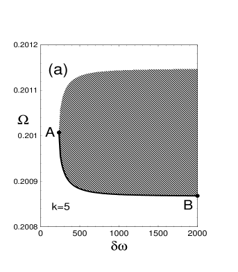
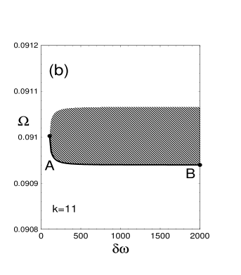
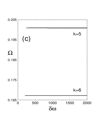
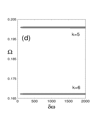
Figure 8. The probability of generation of unwanted states, $P$, at different values of $\delta\omega$ and $\Omega$. In the hatched regions $P<P_{0}$. The different pictures (a) - (d) indicate the different regions in $\Omega$ in different scales. (a), (b), (c) $P_{0}=10^{-5}$; (d) $P_{0}=10^{-4}$. $N=10$.

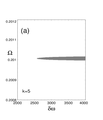
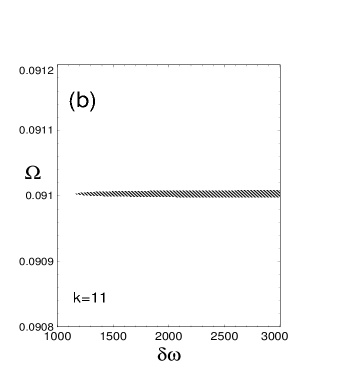
Figure 9. (a) The same as in Fig. 8a but for $N=1000$. (b) The same as in Fig. 8b but for $N=1000$. The scale in $\delta\omega$ shifted to the larger values in comparison with Figs. 8a, 8b.

Figure 10. The exact solution for the probability of generation of unwanted states, $P$, for the parameters, which correspond to: (a) curve AB in Fig. 8a; (b) curve AB in Fig. 8b. The dashed lines indicate the solution obtained by the perturbation theory. $N=10$.

From Figs. 8(c,d) one can see that the sizes of the hatched areas are small, much smaller than the areas between the neighboring hatched regions. The total size of the hatched regions is mostly defined by the probability, $P_{0}$, of tolerant error which can be corrected using additional error correction codes. From comparison of Fig. 8c for $P_{0}=10^{-5}$ and Fig. 8d for $P_{0}=10^{-4}$ one can see that the sizes of the hatched regions increase with $P_{0}$ increasing. The coordinate of the point A in $\Omega$ is $\Omega=\Omega^{[k]}$, where the values of $k$ are indicated in the figures.

In almost all quantum algorithms the phase of the wave function is important. We numerically compared the phase of the wave function on the boundaries of the hatched regions in Figs. 8(a,b) with the phase in the centers of these regions, (where $\Omega$ satisfies $2\pi k$ condition, see Eq. (46), $k=5$ and $k=11$) at fixed $\delta\omega$. The deviation in phase is only $\sim 0.15\%$. This is much less that the corresponding change in the probabilities of errors (by several orders).

In Figs. 9(a,b) we plot the same as in Figs. 8(a,b) but for $N=1000$. One can see that increasing the number of qubits increases the errors and the sizes of the hatched areas decrease considerably. From Figs. 8(a-d) and 9(a-b) one can see that even when the values of $\Omega$ satisfy $2\pi k$-method (position of the point A in $\Omega$ in Figs. 8(a,b) and extreme left points of the hatched regions in Figs. 8(c,d) and 9(a,b)) the error can be relatively large because of the non-resonant processes. From comparison of Figs. 8(a,b) for $N=10$ with Figs. 9(a,b) for $N=1000$ one can see that the minimal value of $\delta\omega$ required to make the errors small increases considerably with $N$ increasing.

We now analyze the probability of errors as a function of $\delta\omega$. When the value of $\delta\omega$ is large enough, the probability of error (and the widths of the hatched areas in $\Omega$) becomes practically independent of $\delta\omega$. This is because at $\delta\omega\gg 1$ and at $\varepsilon\gg\mu$ the error is mostly defined by $\varepsilon$, which is independent of $\delta\omega$. As a consequence, one can, for example, estimate the widths of the hatched areas at $\delta\omega\gg 1$ taking into account only the near-resonant transitions (formula (52)).

In order to test our approximate result we solved the problem exactly using the eigenstates of the matrices ${\mathcal{H}}^{(n)}$, $n=1,\dots M$, for the parameters which correspond to the lower boundary of the hatched regions in the Figs. 8a and 8b (curves AB). In Figs. 10a and 10b we compare the total probability of errors, $P$, obtained using the exact and approximate solutions. One can see again, as in Figs. 6a and 6b, that there is a good correspondence between the exact and approximate solutions. A similar correspondence can be demonstrated for other points of the parametric space ($\delta\omega,\,\Omega$) when the conditions $\Omega\ll J\ll\delta\omega$ are satisfied.

10. A classical Hamiltonian for quantum computation

In this section we demonstrate that the process of quantum computation, including creation of the entanglement, the dynamics of quantum controlled operations, and the dynamics of complicated quantum algorithms can be modeled using classical Hamiltonians. That is not surprising because the basic quantum equations (12) are $c$-number equations and can be formally considered as an effective classical system of equations. The above results show that in some cases, effective classical Hamiltonians can be used for simulation of quantum logic operations even for large number of qubits. We present here the corresponding effective classical Hamiltonian and the Hamiltonian equations of motion in explicit form.

Formally, we can represent the solution of the Schrödinger equation for the Hamiltonian (2)-(4) in the form: $\Psi(t)=\sum^{2^{N}-1}_{n=0}c_{n}(t)|n\rangle$, where $|n\rangle$ and $E_{n}$ are the eigenfunctions and the eigenvalues of the Ising part of the Hamiltonian in (2) in the $z$-representation,

(62) $$\hat{H}_{0}|n\rangle=E_{n}|n\rangle.$$

The complex coefficients, $c_{n}(t)$, satisfy the equations,

(63) $$i\dot{c}_{n}(t)=E_{n}c_{n}(t)+\sum_{k=0}^{2^{N}-1}{V}_{n,k}(t)c_{k}(t),$$

where,

(64) $${V}_{n,k}=\langle n|{V}(t)|k\rangle,$$

and ${V}(t)$ is the interaction Hamiltonian in (2).

Equation (63) can be written in Hamiltonian form:

(65) $$i\dot{c}_{n}={{\delta H_{cl}}\over{\delta c^{*}_{n}}},\qquad i\dot{c}^{*}_{n}=-{{\delta H_{cl}}\over{\delta c_{n}}},$$

where $H_{cl}$ is the Hamiltonian of the equivalent “classical” system,

(66) $$H_{cl}=\sum_{n=0}^{2^{N}-1}E_{n}|c_{n}|^{2}+\sum_{n,p=0}^{2^{N}-1}c_{n}^{*}V_{n,p}c_{p}.$$

Instead of using complex “classical” variables, $c_{n}$ and $c^{*}_{n}$, one can introduce the following real “classical” variables: a “coordinate”, $x_{n}$, and a “momentum”, $p_{n}$, using, for example, the canonical transformation,

(67) $$x_{n}={{1}\over{\sqrt{2}}}(c_{n}+c_{n}^{*}),\qquad p_{n}=-{{i}\over{\sqrt{2}}}(c_{n}-c_{n}^{*}).$$

Using $x_{n}$ and $p_{n}$, Eqs. (65) take the familiar classical Hamiltonian form,

(68) $$\dot{x}_{n}={{\delta H_{cl}}\over{\delta p_{n}}},\qquad\dot{p}_{n}=-{{\delta H_{cl}}\over{\delta x_{n}}},$$

where the equivalent classical Hamiltonian is,

(69) $$H_{cl}(x_{n},p_{n},t)=\sum_{n=0}^{2^{N}-1}{{E_{n}}\over{2}}(x^{2}_{n}+p^{2}_{n})+{{1}\over{2}}\sum_{n,k=0}^{2^{N}-1}(x_{n}-ip_{n})V_{n,k}(x_{k}+ip_{k}).$$

The Hamiltonian (69) can be written in the form,

(70) $$H_{cl}(x_{n},p_{n},t)=\sum_{n=0}^{2^{N}-1}{{E_{n}}\over{2}}(x^{2}_{n}+p^{2}_{n})+$$

$${{1}\over{2}}\sum_{n,k=0}^{2^{N}-1}[x_{n}{\it Re}(V_{n,k})x_{k}+p_{n}{\it Re}(V_{n,k})p_{k}+2p_{n}{\it Im}(V_{n,k})x_{k}],$$

where we used the relations: $V_{n,k}=V^{*}_{k,n}$, and ${\it Re}(V_{n,k})={\it Re}(V_{k,n})$, ${\it Im}(V_{n,k})=-{\it Im}(V_{k,n})$. The corresponding classical Hamiltonian equations follow from (68) and (70),

(71) $$\dot{x}_{n}=E_{n}x_{n}+\sum_{k=0}^{2^{N-1}}[{\it Re}(V_{n,k})p_{k}+2{\it Im}(V_{n,k})x_{k}],$$

$$\dot{p}_{n}=-E_{n}p_{n}-\sum_{k=0}^{2^{N-1}}[{\it Re}(V_{n,k})x_{k}-2{\it Im}(V_{n,k})p_{k}].$$

For example, the Hamiltonian (70) can be used to calculate the dynamics of the quantum Hamiltonian (2). In this case, the matrix elements, $V_{n,k}\not=0$ only for those states $|n\rangle$ which differ from the state $|k\rangle$ by a single-spin transitions, and are zero otherwise.

Solutions of Eqs. (70) satisfy the normalization condition,

(72) $$\sum_{n=0}^{2^{N}-1}[x^{2}_{n}(t)+p^{2}_{n}(t)]=1.$$

Eqs. (70) describe the Hamiltonian dynamics of $2^{N}$ classical “generalized” one-dimensional oscillators. Each of these oscillators is described by two canonically conjugate variables, $x_{n}$ and $p_{n}$. One can see that $2^{N}$ classical harmonic oscillators can simulate the behavior of $N$ interacting quantum qubits, including the dynamics of quantum entanglement, complicated quantum logic gates, and quantum algorithms.

Conclusion

In this paper, we developed an approach, based on small parameters, for the simulation of simple quantum logic operations in a nuclear spin quantum computer with large number of qubits. We considered a quantum computer which is a one-dimensional nuclear spin chain placed in a slightly non-uniform magnetic field, oriented in a direction chosen to suppress the dipole interaction between spins. We took into consideration the Ising interaction between neighboring qubits. Quantum logic operations are implemented by applying resonant electromagnetic pulses to the nuclear spin chain. The electromagnetic pulse which is resonant to a selected qubit is non-resonant for all other qubits. This raises the problem of minimizing the influence of unwanted non-resonant effects in the process of performing a quantum protocol.

We simulate the creation of the long-distance entanglement between remote qubits, $(N-1)$-st and $0$-th, in a nuclear spin quantum computer having a large number of qubits (up to 1000). We used two essential assumptions:
1. The nuclear spin chain is prepared initially in its ground state.
2. The frequency difference between the neighboring spins due to the inhomogeneity of the external magnetic field, $\delta\omega$, is much larger than the Ising interaction constant, $J$, and $J$ is much larger than the Rabi frequency, $\Omega$, i. e. $\Omega\ll J\ll\delta\omega$. Using these assumptions, we developed a numerical method which allowed us to simulate the dynamics of quantum logic operations taking into consideration all quantum states with the probability no less that $P=10^{-6}$. For the case when the $2\pi k$ condition is satisfied (the $\pi$-pulse for the resonant transition is at the same time a $2\pi k$-pulse for non-resonant transitions), we obtained an analytic solution for the evolution of the nuclear spin chain. In the case of small deviations from the $2\pi k$ condition, the error accumulates and the numerical simulations are required. These results are presented in sections 8 and 9.

The main results of our simulations are the following:
1. The unwanted states exhibit a band structure in their probability distributions. There are two main “bands” in the probability distribution of unwanted states. The unwanted states in these “bands” have significantly different probabilities, $P_{low}/P_{upper}\sim 10^{-3}$. Each of these two bands have their own structures.
2. A typical unwanted state is a state of highly correlated spin excitations. An important fact is that the unwanted states with relatively high probability include high energy states of the spin chain (many-spin excitations).
3. The method developed allowed us to study the generation of unwanted states and the probability of the desired states as a function of the distortion of rf pulses. This can be used to formulate the requirements for acceptable errors in quantum computation.

The results of this paper can be used to design experimental implementations of quantum logic operations and to estimate (benchmark) the reliability of experimental quantum computer devices. Our approach can be extended to simulations of simple quantum arithmetic operations and fragments of quantum algorithms. These simulations are now in progress.

References

- [1] G.P. Berman, G.D. Doolen, V.I. Tsifrinovich, Superlattices and Microstructures 27, 89 (2000).
- [2] B.E. Kane, Nature 393, 133 (1998).
- [3] G.P. Berman, G.D. Doolen, V.I. Tsifrinovich, Phys. Rev. Lett. 84, 1615 (2000).
- [4] D. Loss, D.P. DiVincenzo, Phys. Rev. A 57, 120 (1998).
- [5] R. Vrijen, E. Yablonovich, K. Wang, H.W. Jiang, A. Balandin, V. Roychowdhury, T. Mor, D. DiVincenzo, Phys. Rev. A 62, 2306 (2000).
- [6] Y. Nakamura, C.D. Chen, J.S. Tsai, Phys. Rev. Lett. 79, 2328 (1997).
- [7] Y. Nakamura, Yu.A. Pashkin, J.S. Tsai, Nature 398, 786 (1999).
- [8] N.A. Gershenfeld, I.L. Chuang, Science 275, 350 (1997).
- [9] D.G. Cory, A.F. Fahmy, T.F. Havel, Proc. Natl. Acad. Sci. USA 94, 1634 (1997).
- [10] F. Yamaguchi, Y. Yamamoto, Microelectronic Engineering 47, 273 (1999).
- [11] G.P. Berman, G.D. Doolen, G.D. Holm, V.I. Tsifrinovich, Phys. Lett. A 193, 444 (1994).
- [12] I.L. Chuang, N.A. Gershefeld, M. Kubinec, Phys. Rev. Lett. 80, 3408 (1998).
- [13] G.P. Berman, G.D. Doolen, R. Mainieri, V.I. Tsifrinovich, Introduction to Quantum Computers, World Scientific Publishing Company, Singapore, (1998).
- [14] N.N. Bogolubov, Selected Works, Part I. Dynamical Theory, Gordon & Breach Science Pub., (1990).
- [15] A.J. Lichtenberg and M.A. Liberman, Regular and Stochastic Motion, Springer-Verlag, New York, (1983).
- [16] G.M. Zaslavsky, Chaos in Dynamic Systems, Harwood Academic Pub., (1985).
- [17] G.P. Berman, D.K. Campbell, V.I. Tsifrinovich, Phys. Rev. B 55, 5929 (1997).
- [18] G.P. Berman, G.D. Doolen, and V.I. Tsifrinovich Phys. Rev. A 61, 2307 (2000).
- [19] L. D. Landau, E. M. Lifshits, Quantum Mechanics: Non-Relativistic Theory, Pergamon Press, Oxford, New York, (1965).