Fidelity and the communication of quantum information

Abstract

We compare and contrast the error probability and fidelity as measures of the quality of the receiver’s measurement strategy for a quantum communications system. The error probability is a measure of the ability to retrieve classical information and the fidelity measures the retrieval of quantum information. We present the optimal measurement strategies for maximising the fidelity given a source that encodes information on the symmetric qubit-states.

I Introduction

The principles governing the communication of information by a quantum channel are now well-known [1, 2, 3]. The transmiting party (Alice) selects from a set of signal states $\left|\psi_{j}\right\rangle$ and uses a string of these to encode her message. These states are known to the receiving party (Bob) who also knows the a priori probabilities $p_{j}$ for selection of each of the signal states. Bob’s problem is to decide upon an optimal detection strategy. His choice of strategy will depend on the way in which the information he receives is to be used. In mathematical terms, Bob must choose a strategy so as to extremise some function of his measurement outcomes and commonly occurring examples are the minimum error probability or minimum Bayes cost [1, 2, 3, 4, 5] and the accessible information [6, 7, 8, 9, 10]. These quantities determine the quality of Bob’s strategy for recovering the classical information associated with Alice’s selection of the transmitted state.

In this paper we will be concerned with a different measure of Bob’s detection strategy. This quantity, which we refer to as the fidelity, determines Bob’s ability to access the quantum information contained in Alice’s signal. The fidelity depends on Bob’s choice of measurement strategy and also on his subsequent selection of a new quantum state. The extent to which the selected state matches that chosen by Alice will determine Bob’s ability to reconstruct the selected quantum state. We will introduce the fidelity and compare its properties with those of the more familiar error probability in the following section. At this stage, we can motivate our idea by considering the familiar problem of eavesdropping in quantum key distribution [11]. The error probability and fidelity relate, in this case, to the two principal factors in assessing any eavesdropping strategy. The error probability is simply the probability that the eavesdropper will fail to learn the state selected by Alice, while the fidelity is the probability that the state selected by the eavesdropper for transmission to Bob will appear to Bob as the state selected by Alice. In this way, error probability is related to the security of the classical information encoded by Alice and the fidelity is related to the likelihood of escaping detection [12].

We have not been able to find general criteria for maximising the fidelity. This maximum fidelity was introduced by Fuchs [13] who referred to it as the accessible fidelity. For a special class of qubit-states known as the symmetric states, however, we have been able to derive the strategy that maximises the fidelity. The measurement part of the optimal strategy is not unique, but includes the strategy that also minimises the error probability [5].

II Fidelity and error probability

In a quantum communications channel, Bob’s problem is to distinguish between the set of possible signal states, $\left|\psi_{j}\right\rangle(j=1,...M)$, that Alice may have sent. He does this by performing a measurement the results of which are associated with the POM elements [1, 14] $\hat{\pi}_{k}$. There is, of course, no particular reason for the number of possible measurement outcomes to equal M, the number of possible signal states. The probability that Bob observes the result ‘k’ given that Alice selected the state $\left|\psi_{j}\right\rangle$ is

$$P(k|j)=\langle\psi_{j}|\hat{\pi}_{k}|\psi_{j}\rangle.$$ (1)

If Bob wishes to determine the signal state then the probability that he will do so correctly is

$$P_{\rm c}=\sum_{j=1}^{M}P(j|j)p_{j}=\sum_{j=1}^{M}\langle\psi_{j}|\hat{\pi}_{j}|\psi_{j}\rangle p_{j}.$$ (2)

This quantity is a measure of the success of Bob’s strategy at recovering Alice’s (classical) choice of signal state. The error probability is simply $1-P_{\rm c}$:

$$P_{\rm e}=1-\sum_{j=1}^{M}\langle\psi_{j}|\hat{\pi}_{j}|\psi_{j}\rangle p_{j}.$$ (3)

Necessary and sufficient conditions are known for minimising $P_{\rm e}$ (or maximising $P_{\rm c}$) [1, 2, 3, 4] although very few explicit examples of the required POM elements have been given. Some of these minimum error POMs have recently been implemented optically [15, 16, 17].

The fidelity is more closely related to the retrieval of the quantum information ‘$\left|\psi_{j}\right\rangle$’. As a physical picture, consider Bob to be operating some relay station in a communications channel. He must measure the signal and then, on the basis of his measurement, he selects a state to retransmit. The fidelity is then a measure of how well the selected state matches the original signal state selected by Alice. We can see this by considering one of the possible sequence of events. Let us suppose that Alice has sent the signal state $\left|\psi_{j}\right\rangle$ and that Bob measurement has given the result ‘k’ corresponding to the POM element $\hat{\pi}_{k}$. He then selects a state, $\left|\phi_{k}\right\rangle$, that depends on the measurement result, for retransmission. The simplest question that we can ask, to assess the retransmitted state, is “is this state $\left|\psi_{j}\right\rangle$ ?”. The probability that this question will be answered in the affirmative is just the modulus squared overlap of the signal state and the retransmitted state, $|\langle\psi_{j}|\phi_{k}\rangle|^{2}$. The a priori probability that the retransmitted state will pass this test is the fidelity

$$F=\sum_{j=1}^{M}\sum_{k}|\langle\psi_{j}|\phi_{k}\rangle|^{2}\langle\psi_{j}|\hat{\pi}_{k}|\psi_{j}\rangle p_{j}.$$ (4)

This quantity determines the quality of the measurement-retransmission strategy adopted by Bob. The strategy adopted by Bob depends on both his choice of measurement (associated with the POM elements $\hat{\pi}_{k}$) and the selection of the associated retransmission states ($\left|\phi_{k}\right\rangle$). A large value of F corresponds to a good strategy while a smaller value indicates a less good one. The strategy that best extracts the quantum information will be the one that gives the maximum fidelity. The general principles governing the maximum fidelity are unknown to us although the maximum fidelity, the associated measurement and retransmission states have been derived for a special case [13]. We will present strategies for maximising the fidelity for a wider set of possible signal states (the symmetric qubit-states) in section IV.

III Symmetric states

The symmetric states were introduced for the problems of state discrimination by Ban et. al. [5]. These states, $\left|\psi_{j}\right\rangle$, are generated from a single state, $\left|\psi_{1}\right\rangle$, by the action of a unitary operator $\hat{V}$:

$$\left|\psi_{j}\right\rangle=\hat{V}^{j-1}\left|\psi_{1}\right\rangle.$$ (5)

These M states are said to be symmetrical if they are a priori equally likely to have been selected and

$$\hat{V}^{M}=\hat{I}$$ (6)

so that $\left|\psi_{j+M}\right\rangle=\left|\psi_{j}\right\rangle$ [18].

The minimum error probability occurs [5] if we adopt the so-called square-root measurement [19, 20, 21] for which the M POM elements are

$$\hat{\pi}_{k}=\hat{\Phi}^{-1/2}\left|\psi_{k}\right\rangle\left\langle\psi_{k}\right|\hat{\Phi}^{-1/2},$$ (7)

where

$$\hat{\Phi}=\sum_{j=1}^{M}\left|\psi_{j}\right\rangle\left\langle\psi_{j}\right|.$$ (8)

The resulting minimum error probability is then

$$P_{\rm e}^{\rm min}=1-|\langle\psi_{1}|\hat{\Phi}^{-1/2}|\psi_{1}\rangle|^{2}.$$ (9)

In this paper we will obtain the maximum fidelity for any symmetric states of a single qubit. We can represent these states in terms of the orthonormal eigenstates, $\left|\pm\right\rangle$ of the unitary operator

$$\hat{V}={\rm exp}\left[i{{2\pi}\over{M}}\left|-\right\rangle\left\langle-\right|\right].$$ (10)

This operator clearly satisfies the requirement Eq. (6) for a symmetric set of states. Our M, equiprobable symmetric states are

$$\left|\psi_{j}\right\rangle={\rm cos}\left({\theta\over 2}\right)\left|+\right\rangle+{\rm exp}\left(i{{2\pi}\over{M}}(j-1)\right){\rm sin}\left({\theta\over 2}\right)\left|-\right\rangle,\quad(0\leq\theta\leq{\pi\over 2}).$$ (11)

It is helpful to picture these states on the Bloch sphere (see Fig. 1).

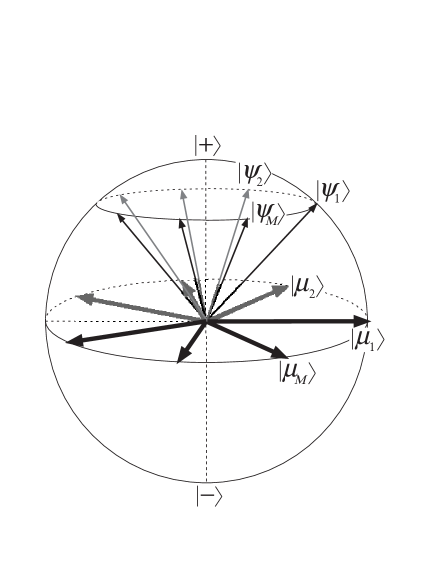
FIG. 1.: The symmetric set of states $\{\left|\psi_{j}\right\rangle\}$. The square root measurement has POM elements that are proportional to projectors onto the states $\{\left|\mu_{j}\right\rangle\}$. This measurement minimises the average error probability for distinguishing between the states.

Each of the states is represented by a point on the surface of the sphere with the polar coordinates, $\theta$ and $\phi$, corresponding to $\theta$ and $2\pi j/M$ respectively in (Eq. 11). The symmetric states lie on a single circle of the Bloch sphere at the latitude $\pi/2-\theta$. For this set of symmetric states the minimum error probability is obtained by means of a POM with elements

$$\hat{\pi}_{j}={2\over M}\left|\mu_{j}\right\rangle\left\langle\mu_{j}\right|,$$ (12)

where

$$\left|\mu_{j}\right\rangle={1\over{\sqrt{2}}}\left[\left|+\right\rangle+{\rm exp}\left(i{{2\pi}\over{M}}(j-1)\right)\left|-\right\rangle\right].$$ (13)

These states correspond to points on the equator of the Bloch sphere at the same longitude ($\phi$ - coordinate) as the corresponding signal states $\left|\psi_{j}\right\rangle$ (see Fig. 1). The associated minimum error probability is

$$P_{\rm e}^{\rm min}=1-{1\over M}\left(1+{\rm sin}\theta\right).$$ (14)

As $\theta$ varies between 0 and $\pi/2$ this error probability varies between $1-1/M$ and $1-2/M$. These values correspond to guessing the value ‘j’ when the states all correspond to the single ket $\left|+\right\rangle$ and the minimum attainable error probability for symmetric states [4, 16] which occurs when the symmetric states lie on the equator of the Bloch sphere.

In the following section we establish the maximum fidelity attainable for this ensemble of states.

IV Maximum fidelity

In seeking to maximise the fidelity it is helpful to write it in the form [13]

$$F=\sum_{k}\langle\phi_{k}|\hat{O}_{k}|\phi_{k}\rangle,$$ (15)

where $\hat{O}_{k}$ is the Hermitian operator

$$\hat{O}_{k}={1\over M}\sum_{j=1}^{M}|\psi_{j}\rangle\langle\psi_{j}|\hat{\pi}_{k}|\psi_{j}\rangle\langle\psi_{j}|.$$ (16)

The selection of the retransmission states $\left|\phi_{k}\right\rangle$ is now straightforward. The best state to select will be the eigenstate of $\hat{O}_{k}$ having the largest eigenvalue and the corresponding maximum fidelity is the sum of the maximum eigenvalues of the operators $\hat{O}_{k}$ [13].

The problem of maximising F is now simply one of selecting the POM or POMs that produce the largest eigenvalue sum. Naturally, there are constraints associated with the fact that our POM elements must be Hermitian, positive-semidefinite and must sum to the identity. In seeking the optimal POM, it is sufficient to consider only rank-one elements correponding to weighted projectors onto pure states [22]. The (rank-one) POM elements can be written in the form

$$\hat{\pi}_{k}=2w_{k}\left[{\rm cos}\left({\theta_{k}\over 2}\right)\left|+\right\rangle+{\rm e}^{i\phi_{k}}{\rm sin}\left({\theta_{k}\over 2}\right)\left|-\right\rangle\right]\left[{\rm cos}\left({\theta_{k}\over 2}\right)\left\langle+\right|+{\rm e}^{-i\phi_{k}}{\rm sin}\left({\theta_{k}\over 2}\right)\left\langle-\right|\right]$$ (17)

or, more simply, as the matrix

$$\hat{\pi}_{k}=w_{k}\left(\begin{array}[]{cc}1+\cos{\theta_{k}}&{\rm e}^{-i\phi_{k}}\sin{\theta_{k}}\\ {\rm e}^{i\phi_{k}}\sin{\theta_{k}}&1-\cos{\theta_{k}}\end{array}\right),$$ (18)

where the basis states $\left|+\right\rangle$ and $\left|-\right\rangle$ correspond to the column vectors $(1,0)^{T}$ and $(0,1)^{T}$ respectively. Here, $w_{k}$ is a weight factor bounded by $0\leq w_{k}\leq 1$. The requirement that the POM elements should sum to the identity places restrictions in the allowed values of the parameters $\theta_{k}$, $\phi_{k}$ and $w_{k}$. These take the form:

$$\sum_{k}w_{k}=1,$$ (19)

$$\sum_{k}w_{k}\cos{\theta_{k}}=0,$$ (20)

$$\sum_{k}w_{k}{\rm e}^{i\phi_{k}}\sin{\theta_{k}}=0.$$ (21)

Our first task is to obtain the greater of the two eigenvalues for each of the operators $\hat{O}_{k}$. Evaluating the sum in Eq. (16) and writing the resulting operator in matrix form gives

$$\hat{O}_{k}={w_{k}\over 2}\left(\begin{array}[]{cc}(1+\cos{\theta})(1+\cos{\theta}\cos{\theta_{k}})&{1\over 2}\sin^{2}{\theta}\sin{\theta_{k}}({\rm e}^{-i\phi_{k}}+\delta_{M,2}{\rm e}^{i\phi_{k}})\\ {1\over 2}\sin^{2}{\theta}\sin{\theta_{k}}({\rm e}^{i\phi_{k}}+\delta_{M,2}{\rm e}^{-i\phi_{k}})&(1-\cos{\theta})(1+\cos{\theta}\cos{\theta_{k}})\end{array}\right),$$ (22)

where $\delta_{M,2}$ is the usual Kronecker delta. We see that this matrix has one of two possible forms, one if $M>2$ and one if $M=2$. It is simplest to deal these two cases separately.

A Case 1: $M>2$

If we have more than two signal states then the operator Eq. (22) reduces to

$$\hat{O}_{k}={w_{k}\over 2}\left(\begin{array}[]{cc}(1+\cos{\theta})(1+\cos{\theta}\cos{\theta_{k}})&{1\over 2}\sin^{2}{\theta}\sin{\theta_{k}}{\rm e}^{-i\phi_{k}}\\ {1\over 2}\sin^{2}{\theta}\sin{\theta_{k}}{\rm e}^{i\phi_{k}}&(1-\cos{\theta})(1+\cos{\theta}\cos{\theta_{k}})\end{array}\right).$$ (23)

The two eigenvalues of this matrix are

$$\nu_{\pm}(\theta_{k})={w_{k}\over 2}\left\{1+\cos{\theta}\cos{\theta_{k}}\pm\left[\cos^{2}{\theta}(1+\cos{\theta}\cos{\theta_{k}})^{2}+{1\over 4}\sin^{4}{\theta}\sin^{2}{\theta_{k}}\right]^{1/2}\right\},$$ (24)

so the maximum value of the fidelity has the form

$$F=\sum_{k}\nu_{+}(\theta_{k})={1\over 2}+{1\over 2}\sum_{k}w_{k}\left[\cos^{2}{\theta}(1+\cos{\theta}\cos{\theta_{k}})^{2}+{1\over 4}\sin^{4}{\theta}\sin^{2}{\theta_{k}}\right]^{1/2},$$ (25)

where we have used Eqs. (19) and (20). Our remaining task is to maximise this quantity subject to the constraints that the operators $\hat{\pi}_{k}$ form a POM Eqs. (19-21). The natural approach to tackling such constrained extremisation problems is to use Lagrange’s method of undetermined multipliers. Before performing this maximisation we note that the maximum fidelity Eq. (25) does not depend on the phases $\phi_{k}$. This means that the contribution to the fidelity will be the same for each POM element having the same value of $\theta_{k}$. Hence we can easily impose the constraint Eq. (21) by choosing a POM with N elements for each distinct value of $\theta_{k}$ satisfying the simpler condition

$$\sum_{l=1}^{N}w_{l}(k){\rm e}^{i\phi_{l}}=0,$$ (26)

where $w_{l}(k)$ are the weights associated with the $N$ POM elements for which $\theta=\theta_{k}$. Hence we will not impose the constraint Eq. (21) in our variational calculation. In order to impose the remaining constraints, Eqs. (19) and (20), we introduce the zero-valued quantities

$$G_{1}=\sum_{k}w_{k}-1,$$ (27)

and

$$G_{2}=\sum_{k}w_{k}\cos{\theta_{k}}.$$ (28)

The extrema of the fidelity will be given by the stationary points of the function

$$H=F+\lambda_{1}G_{1}+\lambda_{2}G_{2}$$ (29)

under independent variation of the parameters $\theta_{k}$ and $w_{k}$. Here $\lambda_{1}$ and $\lambda_{2}$ are the undetermined multipliers.

The stationarity condition for variation of H with respect to $w_{k}$ gives

$${{\partial H}\over{\partial w_{k}}}={1\over 2}\left[\cos^{2}{\theta}(1+\cos{\theta}\cos{\theta_{k}})^{2}+{1\over 4}\sin^{4}{\theta}(1-\cos^{2}{\theta_{k}})\right]^{1\over 2}+\lambda_{1}+\lambda_{2}\cos{\theta_{k}}=0.$$ (30)

while variation with respect to $\theta_{k}$ gives

$${{\partial H}\over{\partial\theta_{k}}} = -\sin{\theta_{k}}{w_{k}\over 2}\left\{\left[\cos^{2}{\theta}(1+\cos{\theta}\cos{\theta_{k}})^{2}+{1\over 4}\sin^{4}{\theta}(1-\cos^{2}{\theta_{k}})\right]^{-{1\over 2}}\left[\cos^{3}{\theta}+\cos{\theta_{k}}\left(\cos^{4}{\theta}-{1\over 4}\sin^{4}{\theta}\right)\right]+2\lambda_{2}\right\}$$ (31)

$$= 0.$$ (32)

The possible solutions of Eq. (32) are (i) $w_{k}=0$ corresponding to uninteresting zero POM elements, (ii) ${\rm sin}\theta_{k}=0$, corresponding to POM elements that are proportional to $\left|+\right\rangle\left\langle+\right|$ and $\left|-\right\rangle\left\langle-\right|$, and (iii) the function in curly parentheses is zero. This final condition reduces, by use of Eq. (30) to

$$\cos{\theta_{k}}={{4\lambda_{1}\lambda_{2}-\cos^{3}{\theta}}\over{\cos^{4}{\theta}-{1\over 4}\sin^{4}{\theta}-4\lambda_{2}^{2}}}=\cos\Theta.$$ (33)

which has only one solution.

Remarkably, we can conclude that the strategy for achieving the maximum fidelity depends only on three possible values of $\theta_{k}$, these being 0, $\pi$ and the, yet to be determined, $\Theta$. Rather than continue with our undetermined multipliers, the simplest way to proceed is to reformulate the problem in terms of the fidelity F with the constraints imposed. We do this by specifying $N+2$ possible POM elements corresponding to the required values (0, $\pi$ and $\Theta$) of $\theta_{k}$:

$$\hat{\pi}_{0}=w_{0}\left(\begin{array}[]{cc}2&0\\ 0&0\end{array}\right),$$ (34)

$$\hat{\pi}_{\pi}=w_{\pi}\left(\begin{array}[]{cc}0&0\\ 0&2\end{array}\right),$$ (35)

$$\hat{\pi}_{l}=w_{l}\left(\begin{array}[]{cc}1+\cos{\Theta}&{\rm e}^{-i\phi_{l}}\sin{\Theta}\\ {\rm e}^{i\phi_{l}}\sin{\Theta}&1-\cos{\Theta}\end{array}\right),\quad(l=1,...,N).$$ (36)

The fidelity is then

$$F={1\over 2}+{w_{0}\over 2}\cos{\theta}(1+\cos{\theta})+{w_{\pi}\over 2}\cos{\theta}(1-\cos{\theta})+W\left[\cos^{2}{\theta}(1+\cos{\theta}\cos{\Theta})^{2}+{1\over 4}\sin^{4}{\theta}(1-\cos^{2}{\Theta})\right]^{{1\over 2}}.$$ (37)

where $W=\sum_{l=1}^{N}w_{l}$. We can impose the constraints, Eqs. (19) and (20), in order to remove $w_{0}$ and $w_{\pi}$ which leaves us with

$$F={1\over 2}+{1\over 2}(1-W)\cos{\theta}-{1\over 2}W\cos^{2}{\theta}\cos{\Theta}+{1\over 2}W\left[\cos^{2}{\theta}(1+\cos{\theta}\cos{\Theta})^{2}+{1\over 4}\sin^{4}{\theta}(1-\cos^{2}{\Theta})\right]^{{1\over 2}}.$$ (38)

Extremising this fidelity to obtain the global maximum value now corresponds to satisfying the conditions

$${{\partial F}\over{\partial W}}={1\over 2}\left\{-\cos{\theta}-\cos^{2}{\theta}\cos{\Theta}+\left[\cos^{2}{\theta}(1+\cos{\theta}\cos{\Theta})^{2}+{1\over 4}\sin^{4}{\theta}(1-\cos^{2}{\Theta})\right]^{{1\over 2}}\right\}=0,$$ (39)

$${{\partial F}\over{\partial\Theta}} = -\sin{\Theta}{W\over 2}\left\{-\cos^{2}{\theta}+\left[\cos^{2}{\theta}(1+\cos{\theta}\cos{\Theta})^{2}+{1\over 4}\sin^{4}{\theta}(1-\cos^{2}{\Theta})\right]^{-{1\over 2}}\left[\cos^{3}{\theta}+\cos{\Theta}(\cos^{4}{\theta}-{1\over 4}\sin^{4}{\theta})\right]\right\}$$ (40)

$$= 0.$$ (41)

The solution ${\rm sin}\Theta=0$ corresponds to the POM elements Eqs. (34) and (35). Combining the remaining non-trivial solution with (Eq. 39) leads to the appealingly simple result that ${\rm cos}\Theta=0$. Hence the fidelity has the form

$$F={1\over 2}(1+\cos{\theta})+{W\over 2}\left[(\cos^{2}{\theta}+{1\over 4}\sin^{4}{\theta})^{1\over 2}-\cos{\theta}\right].$$ (42)

The maximum value that this can take clearly corresponds to setting $W=1$ and hence the global maximum value that the fidelity can take for symmetric qubit-states is

$$F_{\rm max}=1-{1\over 4}\sin^{2}{\theta}.$$ (43)

This takes its maximum value of unity for $\theta=0$. This is reasonable as in this case all the signal states correspond to $\left|+\right\rangle$ and unit fidelity can always be achieved by choosing the single state $\left|+\right\rangle$ for retransmission. The fidelity is a monotonically decreasing function of $\theta$ and takes its smallest value of $3/4$ for $\theta=\pi/2$ [13].

Having determined the maximum value of the fidelity, we now turn our attention to the form of Bob’s strategy for realising this value. The conditions $\Theta=\pi/2$ and $W=1$ tell us that the optimal POM will have $N$ elements of the form

$$\hat{\pi}_{l}=w_{l}\left(\begin{array}[]{cc}1&{\rm e}^{-i\phi_{l}}\\ {\rm e}^{i\phi_{l}}&1\end{array}\right)=w_{l}\left(\left|+\right\rangle+{\rm e}^{i\phi_{l}}\left|-\right\rangle\right)\left(\left\langle+\right|+{\rm e}^{-i\phi_{l}}\left\langle-\right|\right),$$ (44)

where the parameters $w_{k}$ and $\phi_{k}$ satisfy the constraints

$$\sum_{l=1}^{N}w_{l}=1,\quad(0\leq w_{l}\leq 1)$$ (45)

$$\sum_{l=1}^{N}w_{l}{\rm e}^{i\phi_{l}}=0,$$ (46)

corresponding to Eqs. (19) and (20) respectively. The problem of maximising the fidelity does not constrain the choice of POM any further than this and so any POM with elements of the form (Eq. 44) and satisfying the conditions Eqs. (45) and (46) will maximise the fidelity. Important examples include the symmetric POM with elements

$$\hat{\pi}_{l}={1\over N}\left(\begin{array}[]{cc}1&{\rm exp}\left[-i(\alpha+{{2\pi l}\over{N}})\right]\\ {\rm exp}\left[i(\alpha+{{2\pi l}\over{N}})\right]&1\end{array}\right),\quad(N\geq 2)$$ (47)

where $\alpha$ is any desired phase. We note that the choice $N=2$ corresponds to a simple von Neumann measurement. Furthermore, setting $N=M$ and $\alpha=0$ shows that the square-root measurement, with POM elements Eq. (12) can also maximise the fidelity. An example of the states corresponding the POM with elements Eq. (47) is depicted in Fig. 2.

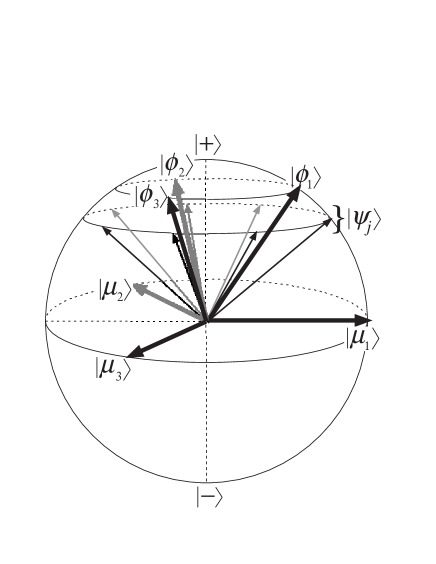
FIG. 2.: Optimal strategy that attains the maximum fidelity. There are various possible optimal measurement strategies as explained in the text. In this figure, the measurement with three outputs $(M=3)$ and $\alpha=0$, and the corresponding retransmission states are shown. The retransmission states are positioned at the same longitude ($\phi$ coordinate) as the corresponding POM elements but are further north than the original signal states.

The retransmission states $\left|\phi_{l}\right\rangle$ that maximise the fidelity correspond to the maximum-eigenvalue eigenstates of the operator Eq. (23) with $\theta_{k}=\Theta=\pi/2$. This operator is

$$\hat{O}_{l}={w_{l}\over 2}\left(\begin{array}[]{cc}1+\cos{\theta}&{1\over 2}{\rm e}^{-i\phi_{l}}\sin^{2}{\theta}\\ {1\over 2}{\rm e}^{i\phi_{l}}\sin^{2}{\theta}&1-\cos{\theta}\end{array}\right)$$ (48)

and the corresponding maximum eigenvalue is

$$\nu_{+}(l)=w_{l}\left(1-{1\over 4}\sin^{2}{\theta}\right).$$ (49)

Solving the for the associated eigenvector gives the required retransmission state associated with the measurement outcome ‘$k$’:

$$\left|\phi_{l}\right\rangle = {1\over{\sqrt{2}}}\left(1+\cos^{2}{\theta}\right)^{-{1\over 2}}\left[\left(1+\cos{\theta}\right)\left|+\right\rangle+{\rm e}^{i\phi_{l}}\left(1-\cos{\theta}\right)\left|-\right\rangle\right]$$ (50)

$$= \cos{\left({\chi}\over{2}\right)}\left|+\right\rangle+{\rm e}^{i\phi_{l}}\sin{\left({\chi}\over{2}\right)}\left|-\right\rangle.$$ (51)

These states are depicted on the Bloch sphere in Fig. 2. They are positioned at the same longitude ($\phi$ coordinate) as the corresponding POM elements but are further north than the original signal states, having a lattitude $\pi/2-\chi$ where

$$\cos{\chi}={2\cos{\theta}\over{1+\cos^{2}{\theta}}}.$$ (52)

We can now summarise our strategies for obtaining the maximum fidelity. Any POM with elements given by Eq. (47) constitutes an optimum measurement. These operators will form a POM if the conditions Eqs. (45) and (46) are satisfied. The fidelity will be maximised if the retransmission state selected on the basis of a the measurement outcome ‘$l$’ has the polar coordinates ($\chi,\phi_{l}$) on the Bloch sphere, with $\chi$ given by Eq. (52).

B Case 2: M=2

If $M=2$ then we have only two possible signal states:

$$\left|\psi_{j}\right\rangle={\rm cos}\left({\theta\over 2}\right)\left|+\right\rangle\pm{\rm sin}\left({\theta\over 2}\right)\left|-\right\rangle.\quad(0\leq\theta\leq{\pi\over 2})$$ (53)

The representation of these states on the Bloch sphere is depicted in Fig. 3.

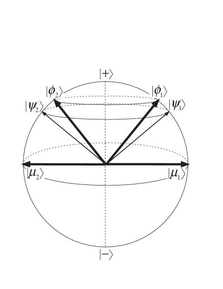
FIG. 3.: The case of two signal states. In this case the optimal solution is unique, and comprises a von Neumann measurement and the retransmission of two nonorthogonal states. The retransmission states are again further north than the original signal states. All the relevant states have the same longitude.

The two states correspond to two points at the same latitude in the northern hemisphere with longitudes separated by $\pi$. For these two states the operator (22) becomes

$$\hat{O}_{k}={w_{k}\over 2}\left(\begin{array}[]{cc}(1+\cos{\theta})(1+\cos{\theta}\cos{\theta_{k}})&\sin^{2}{\theta}\sin{\theta_{k}}\cos{\phi_{k}}\\ \sin^{2}{\theta}\sin{\theta_{k}}\cos{\phi_{k}}&(1-\cos{\theta})(1+\cos{\theta}\cos{\theta_{k}})\end{array}\right),$$ (54)

the eigenvalues of which are

$$\nu_{\pm}(\theta_{k},\phi_{k})={w_{k}\over 2}\left\{1+\cos{\theta}\cos{\theta_{k}}\pm\left[\cos^{2}{\theta}(1+\cos{\theta}\cos{\theta_{k}})^{2}+\sin^{4}{\theta}\sin^{2}{\theta_{k}}\cos^{2}{\phi_{k}}\right]^{1/2}\right\}.$$ (55)

The required greater of the two eigenvalues is clearly maximised by setting $\phi_{k}=0$ or $\pi$. Thus the strategy that maximises the fidelity must comprise only POM elements corresponding to states at the same longitudes as the two signal states.

The maximisation of the fidelity (25) follows the same lines as that for the case $M>2$ and we will only present the main results. The extremisation of the fidelity subject to the constraints (19) and (20) leads to the conclusion that the only possible values for $\theta_{k}$ are $0,\pi$ and one other angle $\Theta$. Repeating the extremisation with these possible values for $\theta_{k}$ leads to the result that $\Theta=\pi/2$ and that this is the value for which the fidelity can attain its maximum value. It follows that the unique measurement strategy for maximising the fidelity with the two possible signal states (53) has the two POM elements

$$\hat{\pi}_{k}={1\over 2}\left(\begin{array}[]{cc}1&(-1)^{k-1}\\ (-1)^{k-1}&1\end{array}\right).$$ (56)

This corresponds to a von Neumann measurement, the two possible outcomes of which correspond to the two orthonormal states

$$\left|\mu_{k}\right\rangle={1\over{\sqrt{2}}}\left(\left|+\right\rangle+(-1)^{k-1}\left|-\right\rangle\right).$$ (57)

This is the strategy that also minimises the error probability if we associate the measurement outcome ‘$k$’ with the signal state $\left|\psi_{k}\right\rangle$. The resulting maximum possible value for the fidelity is

$$F_{\rm max}={1\over 2}\left[1+\left(\cos^{2}{\theta}+\sin^{4}{\theta}\right)^{1\over 2}\right].$$ (58)

This takes its maximum value of unity for both $\theta=0$ and $\theta=\pi/2$. This is reasonable as for $\theta=0$ all the signal states correspond to $\left|+\right\rangle$ and unit fidelity can be achieved by simply retransmitting $\left|+\right\rangle$. For $\theta=\pi/2$ the two signal states (53) are orthogonal and a von Neumann measurement can determine the signal state with certainty. The required retransmission state is then simply the signal state.

The required retransmission states that achieve this maximum fidelity are the eigenstates of the two operators

$$\hat{O}_{k}={1\over 4}\left(\begin{array}[]{cc}(1+\cos{\theta})&(-1)^{k-1}\sin^{2}{\theta}\\ (-1)^{k-1}\sin^{2}{\theta}&(1-\cos{\theta})\end{array}\right),$$ (59)

having the common greater eigenvalue

$$\nu_{+}={1\over 4}\left[1+\left(\cos^{2}{\theta}+\sin^{2}{\theta}\right)^{1\over 2}\right].$$ (60)

These retransmission states are

$$\left|\phi_{k}\right\rangle = {1\over{\sqrt{2}}}\left(\cos^{2}{\theta}+\sin^{4}{\theta}\right)^{-{1\over 4}}\left[\left(\cos^{2}{\theta}+\sin^{4}{\theta}\right)^{1\over 2}-\cos{\theta}\right]^{-{1\over 2}}\left\{\sin^{2}{\theta}\left|+\right\rangle+(-1)^{k}\left[\left(\cos^{2}{\theta}+\sin^{4}{\theta}\right)^{1\over 2}-\cos{\theta}\right]\left|-\right\rangle\right\}$$ (61)

$$= \cos{\left({\chi_{2}}\over{2}\right)}\left|+\right\rangle+(-1)^{k}\sin{\left({\chi_{2}}\over{2}\right)}\left|-\right\rangle$$ (62)

and are depicted on the Bloch sphere in Fig. 3. They have the same longitude as the corresponding POM elements but are again further north than the original signal states having a latitude $\pi/2-\chi_{2}$ where

$$\cos{\chi_{2}}=\cos{\theta}\left(\cos^{2}{\theta}+\sin^{4}{\theta}\right)^{-{1\over 2}}.$$ (63)

This angle also corresponds to a latitude that is south of the optimum for the cases in which $M>2$.

If there are only two possible signal states then the maximum fidelity is achieved by means of the unique strategy of performing the simple von Neumann measurement corresponding to the POM elements (56). The required retransmission states associated with the relevant measurement outcomes have the form given in Eq. (62).

V Conclusion

In a quantum communications channel the signal comprises a known set of quantum states, each with a known a priori probability for transmission. The possibility of selecting non-orthogonal states distinguishes the quantum channel from its classical counterpart and leads to novel technical possibilities including quantum key distribution [11]. It also creates the interesting problem for the receiver of having to select between a number of possible detection strategies. The decision will be informed by the purpose for which the information retrieved is intended. The strategy that minimises the error probability will have the greatest chance of retrieving the number ‘$j$’ associated with the initial classical selection of the signal state. As such it is a measure of the quality of the measurement strategy for retrieving this classical information. The fidelity, however, determines how well a state, selected on the basis of the measurement outcome, will match the originally transmitted signal state. As such it depends on both the choice of measurement strategy and the selection of the associated ‘retransmission’ states. The fidelity measures the quality of the measurement strategy for retrieving $\left|\psi_{j}\right\rangle$ rather than ‘$j$’ and as such is a measure of the receiver’s ability to recover the quantum information in the signal.

The fundamental difference between the error probability and the fidelity may be illustrated with a simple example. Suppose that the $M$ equiprobable signal qubit states are all of the form $\left|+\right\rangle$. In this case, there is no measurement that can decrease the error probability below the value $1-1/M$ obtained by guessing the state. Selecting $\left|+\right\rangle$ as the only retransmission state, however, gives the greatest possible fidelity of unity.

In this paper we have derived the maximum possible fidelity for the symmetric qubit states defined in Eq. (11). This maximum value depends on whether there are two or more than two possible signals states. For more than two signal states there is a wide range of suitable measurement strategies that can achieve the maximum fidelity. This includes the unique strategy that minimises the error probability. For two signal states the only strategy that can achieve the maximum fidelity is that which minimises the error probability. In general, the required retransmission states depend on the measurement outcome but coincide with neither the signal states nor the elements of the measurement POM. It remains an open question as to whether, for all possible states, the strategy that minimises the error probability will always maximise the fidelity. We will return to this question elsewhere.

- [1] C. W. Helstrom, Quantum Detection and Estimation Theory (Academic Press, New York, 1976).
- [2] A. S. Holevo, Probabilistic and Statistical Aspects of Quantum Theory (North-Holland, Amsterdam, 1982).
- [3] O. Hirota, Optical Communication Theory (Morikita, Tokyo, 1985) (in Japanese).
- [4] H. P. Yuen, R. S. Kennedy and M. Lax, IEEE Trans. Inf. Theory IT-21, 125 (1975).
- [5] M. Ban, K. Kurokawa, R. Momose and O. Hirota, Int. J. Theo. Phys. 36, 1269 (1997).
- [6] E. B. Davies, IEEE Trans. Inf. Theory IT-24, 596 (1978).
- [7] C. A. Fuchs and A. Peres, Phys. Rev. A 53, 2038 (1996).
- [8] M. Ban, K. Yamazaki and O. Hirota, Phys. Rev. A 55, 22 (1997).
- [9] M. Osaki, M. Ban and O. Hirota, J. Mod. Opt. 45, 269 (1998).
- [10] M. Sasaki, S. M. Barnett, R. Jozsa, M. Osaki and O. Hirota, Phys. Rev. A 59, 3325 (1999).
- [11] S. J. D. Phoenix and P. D. Townsend, Contemp. Phys. 36, 165 (1995) and references therein.
- [12] There are, of course, more sophisticated strategies available to the eavesdroper than measurement and retransmission and the quality of these will be determined by other measures.
- [13] C. A. Fuchs and M. Sasaki, (to be published).
- [14] A. Peres, Quantum Theory: Concepts and Methods (Kluwer, Academic Publishers, Dordrecht, 1993).
- [15] S. M. Barnett and E. Riis, J. Mod. Opt. 45, 1295 (1997).
- [16] R. B. M. Clarke, V. M. Kendon, A. Chefles, S. M. Barnett, E. Riis and M. Sasaki, Phys. Rev. A (in press).
- [17] M. Fujiwara, J. Mizuno, M. Akiba, T. Kawanishi, S. M. Barnett and M. Sasaki, (to be published).
- [18] We note that we can also accommodate situations in which , for some phase , by replacing with .
- [19] A. S. Holevo, Theory Prob. Appl., vol. 23, 411, June (1978).
- [20] P. Hausladen and W. K. Wootters, J. Mod. Opt. 41, 2385 (1994).
- [21] P. Hausladen, R. Jozsa, B. Schumacher, M. Westmoreland and W. K. Wootters, Phys. Rev. A 54, 1869 (1996).
- [22] The reason for this is that the fidelity is linear in the POM elements and hence rank-two projectors can be included as a pair of rank-one projectors.