Comparative study of the transient evolution of Hanle EIT/EIA resonances.

Abstract

The temporal evolutions of coherent resonances corresponding to electromagnetically induced transparency (EIT) and absorption (EIA)  were observed in a Hanle absorption experiment carried on the $D_{2}$ lines of ⁸⁷Rb vapor by suddenly turning the magnetic field on or off. The main features of the experimental observations are well reproduced by a theoretical model based on Bloch equation where the atomic level degeneracy has been fully accounted for. Similar (opposite phase) evolutions were observed at low optical field intensities for Hanle/EIT or Hanle/EIA resonances. Unlike the Hanle/EIA transients which are increasingly shorter for driving field intensities approaching saturation, the $B\neq 0$ transient of the Hanle/EIT signal at large driving field intensities present a long decay time approaching the atomic transit time. Such counterintuitive behavior is interpreted as a consequence of the Zeno effect.

I Introduction.

Large attention has been paid in recent years to the fascinating properties of macroscopic samples of atoms or molecules prepared in a specific linear combination of quantum states [1]. Such media are said to be coherently prepared and its statistical (macroscopic) description corresponds to a density matrix with nonzero off-diagonal (coherence) terms. A wide variety of physical consequences of coherently prepared media have been observed and many crucial applications achieved [2]. A few examples are: Coherence population trapping (CPT) [3, 4] successfully exploited for sub-recoil laser cooling [5]. Electromagnetically induced transparency (EIT) and the related topic of laser without inversion [6]. Enhancement of optical nonlinearities [7] and efficient frequency generation [8]. Very large dispersion [9] and its application to sensitive magnetometry [10] and optical propagation with slow group velocity [11, 12].

Most experiments and theoretical modelling on CPT, EIT and related coherence effects deal with three level systems in a $\Lambda$ configuration where the two long-living lower levels have different energies. This requires the consideration of two distinct optical fields (coupling and probe fields) acting on either arms of the $\Lambda$ system. However, interesting energy level configurations for coherent spectroscopy purposes can also be obtained using the Zeeman sublevels of a degenerate two-level atomic transition.

The coherent spectroscopy of degenerate two-level systems (DTLS) was recently explored using mutually coherent optical fields [13, 14, 15, 16]. A new coherent effect emerged corresponding to a resonant increase of the atomic absorption. Such effect was designated electromagnetically induced absorption (EIA). EIA is observed in DTLS in closed transitions with a higher degeneracy in the upper level [13, 14]. Recently, coherent resonances in DTLS were used to produce very slow positive and negative [15] group velocity and to obtain “light storage” [17].

A major advantage of the use of DTLS is that a single optical field may be enough to induce coherent effects. Indeed, the two orthogonal polarization components ($\sigma^{+}$ and $\sigma^{-}$) of the same linearly polarized optical wave couple different Zeeman sublevels of the ground and excited state. The Raman resonance condition between ground state sublevels is then automatically reached at perfect ground state degeneracy or destroyed by the application of a static magnetic field. As a result, the atomic response of a DTLS to the excitation by a single optical field with linear polarization presents sharp variations as a function of the magnetic field around zero magnetic field. This is in essence the well known (ground state) Hanle effect [18, 19, 20] intimately connected to the Zeeman optical pumping [21].

CPT and Hanle effects were theoretically and experimentally analyzed within a common frame by Renzoni and coworkers [22]. They studied the hyperfine (open) transitions of the $D_{1}$ line of Na. This work was followed by theoretical investigation of Hanle/CPT resonances in open transitions [23, 24, 25]. Hanle/CPT resonances were also studied on the $D_{1}$ and $D_{2}$ lines of Rb in a vapor cell experiment. Inverted Hanle resonances (increased absorption) were then observed in the case of $F_{g}\rightarrow F_{e}=F_{g}+1$ transitions [26]. These resonances are related to the EIA effect previously reported in [13, 14]. A theoretical investigation of the enhanced absorption Hanle resonances has recently been presented in [27].

The temporal evolution of EIT signals was theoretically analyzed by Li and coworkers [28] and experimentally investigated by Chen et al. [29] for strong coupling field intensity. The low driving field intensity case was initially considered in [30]. The influence of several relaxation mechanisms such as time-of-flight, dephasing collisions and velocity changing collisions was studied in [31]. A refined treatment of the influence of the time-of-flight on the transient atomic response in coherence resonances was discussed in [23, 24].

This paper is concerned with the study of the temporal evolution of the Hanle signal as the Raman resonance condition between the optical field and the ground state Zeeman sublevels is suddenly achieved or destroyed by turning off or on a static longitudinal magnetic field. We focus on the comparison between the temporal evolution of the Hanle/EIT (reduced absorption) and Hanle/EIA (increased absorption) resonances at various driving field intensities. The experiments were carried on the $D_{2}$ lines of Rb in a vapor cell. Although we studied both stable Rb isotopes, only the results concerning ⁸⁷Rb will be presented here. The two cases (Hanle/EIT or Hanle/EIA resonances) can be observed depending on which ground state hyperfine level is excited. As already pointed out [13, 14, 26, 27], the atomic response when the lower alkaline atom ground state hyperfine level is excited corresponds, at the Raman resonance, to increased transparency (EIT). Conversely, the response obtained when the upper ground state hyperfine level is excited results in an inverted Hanle resonance corresponding to an increase of the atomic absorption (EIA). For an EIT type transition, the transient  following the cancellation of the magnetic field can be interpreted as the falling of the atomic system into the uncoupled or dark state (DS). For an EIA type transition, the transient corresponds to the atomic system evolving towards the enhanced absorption state (EAS) [27]. We have also studied the transients occurring when the Raman resonance condition is suddenly modified by the application of a magnetic field producing a Zeeman shift of the ground state sublevels which is larger than the coherence resonance width at low light intensity but smaller than the excited state width. This transient evolution correspond to the system leaving the DS or the EAS in the case of EIT or EIA type transitions respectively.

The experiments are described in the next section of the paper. Section three is devoted to the discussion of the experimental results in view of a theoretical model of the atomic evolution. Section four presents the conclusions of this work.

II Experiment.

The experimental setup scheme is shown in Fig. 1. A $2\ cm$ long glass cell containing a mixture of ⁸⁵Rb and ⁸⁷Rb vapor and no buffer gas was used. The cell was slightly heated above room temperature to obtain around $70\%$ resonant absorption. The cell was placed inside a cylindrical coil for magnetic field control. The coil and the cell were placed inside a cylindrical $\mu$-metal shield to reduce magnetic fields components perpendicular to the cylindrical coil axis to less than $10\ mG$. The atomic sample was illuminated with a $1\ mW$ laser beam issued from an injection locked diode laser (linewidth $<1\ MHz$) whose frequency could be tuned and stabilized along the Rb $D_{2}$ lines ($780\ nm$). The precise laser frequency position was monitored with respect to an auxiliary saturated absorption setup. The laser light was spatially filtered using a $50\ cm$ long single mode optical fiber. The linearly polarized laser propagated along the direction of the magnetic coil axis. The intensity of the light was controlled with neutral density filters. An iris diaphragm placed before the cell defined the beam cross section at the atomic sample. A second diaphragm, with smaller diameter, placed after the cell selects the central part of the transmitted beam. The transmission was monitored with an avalanche photodiode ($100\ MHz$ bandwidth) and recorded in a digitizing oscilloscope.

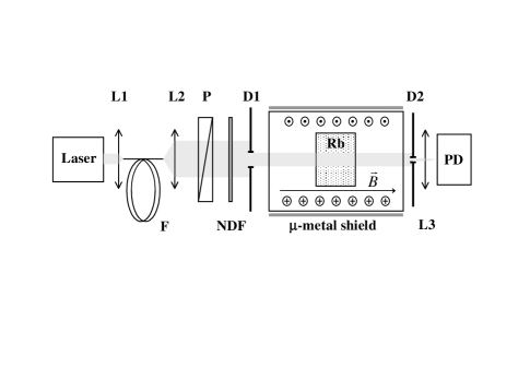
FIG. 1.: Scheme of the experimental setup (L1, L2, L3: lenses, F: mono-mode optical fiber, P: polarizer, NDF: neutral density filter, D1, D2: iris diaphragms, PD: photodiode).

To study the transient behavior of the Hanle/EIT(/EIA) resonances the longitudinal magnetic field was periodically switched between two different constant values $B_{0}=0$ and $B_{1}\simeq 250\ mG$ while observing the temporal variation of the transmitted light power. For this, the coil current was driven by the square-wave output of a signal generator at $10\ kHz$. After being switched on or off the magnetic field reached a new stationary value in approximately $0.5\ \mu s.$ During the recording of the absorption transients, the iris diaphragm placed after the cell had a diameter at least a factor of two smaller than the diameter of the iris placed before the cell and defining the beam cross section. By this means, one ensures that the collected light originates from atoms whose transverse path across the cylindrical light beam is close to a diameter. For these atoms the mean transverse transit time across the beam can be estimated as $\tau=D\left(2k_{B}T/m\right)^{-1/2}$ where $D$ is the beam diameter, $T$ the vapor temperature, $k_{B}$ the Boltzman constant and $m$ the atom mass (For Rb $\tau\simeq 40$ $\mu s$ for $D=1\ cm$  and $T=330\ K$).

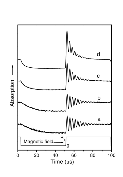
FIG. 2.: Observed transient evolution of the Hanle/EIT resonance in ${}^{87}Rb$ for different driving field intensities $I$. a) $I\simeq 30\ \mu W/cm^{2}$, b) $I\simeq 90\ \ \mu W/cm^{2}$, c) $I\simeq 0.3\%mW/cm^{2}$, d) $I\simeq 0.9\ mW/cm^{2}$. Magnetic field $B_{1}\simeq 250\ mG$. Driving field tuned near the peak of the $5S_{1/2}\left(F=1\right)\rightarrow 5P_{3/2}$ Doppler broadened absorption line.

The transient absorption records obtained for EIT and EIA type transitions are shown in Figs. 2 and 3 respectively. When the magnetic field is switched off, the atomic system evolves exponentially towards a new steady state which corresponds to the DS in the case of an EIT type transition or the EAS in the case of an EIA type transition. A quite different behavior is observed when the magnetic field is suddenly restored. The evolution towards the new steady state is then a damped oscillation at a frequency given by twice the ground state Zeeman frequency produced by the magnetic field. This oscillation corresponds to the Larmor precession of the coherently prepared DS or EAS in the presence of the static magnetic field. Notice the opposite phase corresponding to the EIT and EIA type transitions.

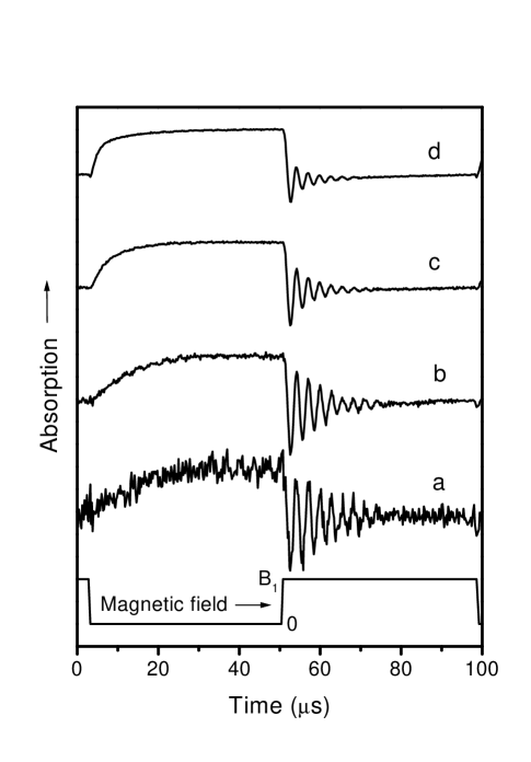
FIG. 3.: Observed transient evolution of the Hanle/EIA resonance in ${}^{87}Rb$ for different driving field intensities $I$. a) $I\simeq 30\ \mu W/cm^{2}$, b) $I\simeq 90\ \ \mu W/cm^{2}$, c) $I\simeq 0.3\%mW/cm^{2}$, d) $I\simeq 0.9\ mW/cm^{2}$. Magnetic field $B_{1}\simeq 250\ mG$. Driving field tuned near the peak $5S_{1/2}\left(F=2\right)\rightarrow 5P_{3/2}$ Doppler broadened absorption line.

Figs. 2 and 3 present the variations with light intensity of the transient evolutions of EIT and EIA type transitions respectively. In these series, the laser beam diameter is kept fixed at $1.3\ cm$ while its intensity is varied with neutral density filters. The plots have been rescaled in order to present the same difference between the two steady states regimes. At all intensities, the transient evolution towards the steady state regime with $B=0$ is well described by an exponential decay. Similar decay times are observed at $B=0$ for a given laser intensity for EIT and EIA type transitions. This is still the case of the $B\neq 0$ transients at low intensities, the damping of the oscillating transients occur with similar characteristic decay rates for the EIT and EIA type transitions. These rates, which are also comparable to the $B=0$ exponential decay rates observed for the same light intensity are of same magnitude than the inverse of the estimated time-of-flight across the light beam. Significant differences between the EIT and EIA transients arise for $B\neq 0$ as the light intensity is increased. In the EIA type transition (Fig. 3) increasing the light intensity results in a faster damping of the oscillating transient. The damping rate of the oscillation closely follows the exponential decay rate of the corresponding $B=0$ transient. The behavior is rather different for the $B\neq 0$ transient in the EIT type transition. In this case the temporal evolution significantly deviates from a single sine-damped oscillation. It is better described by the sum of a sine-damped oscillation plus a non oscillating exponentially decaying term. The characteristic decay rate of this non oscillating term is rather insensitive to the laser intensity and remains comparable to the time-of-flight decay rate. For a quantitative analysis, the observed temporal evolutions were (least square) fitted with the function $y_{1}\left(t\right)=Aexp\left(-\eta_{2}t\right)$ in the case of the $B=0$ transients and with the function $y_{2}\left(t\right)=Cexp\left(-\eta_{1}t\right)+Dexp\left(-\eta_{3}t\right)sin(\beta t+\varphi)$ for the $B\neq 0$ transients ($A,C,D,\eta_{1},\eta_{2},\eta_{3},\beta,\varphi$ are adjustable parameters). Since the $B\neq 0$ transient for the EIA type transition does not show any significant non oscillating term, in this case, coefficient $C$ was taken zero. The fitting functions closely adjust to the data (the differences would be barely observable on the scale of Figs. 2 and 3). The fitted values of the decay rates and the oscillation frequency are plotted in Fig. 4. Notice that $\eta_{0}$ and $\eta_{2}$ are growing functions of the laser intensity $I$ while $\eta_{1}$ remains approximately constant.

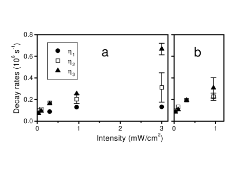
FIG. 4.: Intensity dependence of the exponential decay rate $\eta_{2}$ observed for $B=0$,  the exponential decay rate $\eta_{1}$ of the non oscillating component and the damping rate $\eta_{3}$ of the oscillating component of the transients observed for $B\neq 0$. a) EIT type transition. b) EIA type transition. Light beam diameter at the cell $13\ mm$.

Using the same intensity than in the case of Fig. 2d, we have checked that $\eta_{1}$ is linearly dependent on the inverse diameter of the diaphragm placed before the cell indicating that this decay rate is essentially determined by the atomic time-of-flight (see Fig. 5).

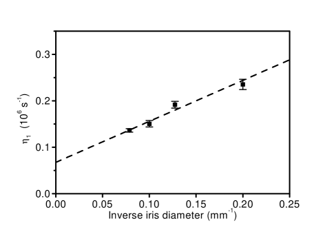
FIG. 5.: Dependence of the decay rate $\eta_{1}$ on light beam diameter. Ligth intensity: $0.9\ mW/cm^{2}$.

III Theoretical analysis and discussion.

The experimental results presented above will be discussed in this section in view of a simple theoretical model of the atomic evolution. We follow the standard density matrix approach using optical Bloch equations and the rotating wave approximation [28]. Several simplifications are made. The atoms are considered at rest and the atomic sample is assumed to be homogeneous. The finite time-of-flight of the atoms through the light beam is taken into account in the calculation through a phenomenological decay rate [30, 31]. The theoretical model does not intend to represent the actual level structure of the $D_{2}$ transitions of ⁸⁷Rb. Instead, we have chosen to analyze two model transitions: $F_{g}=1\rightarrow F_{e}=0$ and $F_{g}=1\rightarrow F_{e}=2$ which are the simplest to correspond to EIT and EIA respectively [14]. The two transitions are considered closed in the sense that the radiative decay of the excited level is exclusively into the ground level.

Following the procedure and notation introduced in [14, 16], we consider an atom at rest with a ground level $g$ and an excited level $e$ with angular momenta $F_{g}$ and $F_{e}$ respectively and energy separation ${}\hbar\omega_{0}$. Spontaneous emission from $e$ to $g$ occurs at a rate $\Gamma$. The finite interaction time is accounted for by the relaxation rate $\gamma$ ($\gamma\ll\Gamma$). The atoms are submitted to the action of a magnetic field $B$ and a classical monochromatic electromagnetic field: $\vec{E}(t)=E\hat{e}\exp(i\omega t)$,    where $\hat{e}$ is a complex unit polarization vector.

Introducing the slowly varying matrix $\sigma=P_{g}\rho P_{g}+P_{e}\rho P_{e}+P_{g}\rho P_{e}\exp\left(-i\omega t\right)+P_{e}\rho P_{g}\exp\left(i\omega t\right)$ (where $\rho$ is the density matrix in the Schrödinger representation and $P_{g}\$and $P_{e}\$are projectors on the ground and excited subspaces respectively), the time evolution of the system (in the rotating wave approximation) obeys:

$$\frac{d\sigma}{dt} = -\frac{i}{\hbar}\left[H_{Z}+\hbar\Delta P_{e}+V,\sigma\right]-\frac{\Gamma}{2}\left\{P_{e},\sigma\right\}$$ (2)

$$+\Gamma\left(2F_{e}+1\right)\sum_{q=-1,0,1}Q_{ge}^{q}\sigma Q_{eg}^{q}-\gamma\left(\sigma-\sigma_{0}\right)$$

where $H_{Z}=(\beta_{g}P_{g}+\beta_{e}P_{e})F_{z}B$ is the Zeeman Hamiltonian ($\beta_{g}$ and $\beta_{e}$ are the ground and excited sate gyromagnetic factors and $F_{z}$ is the total angular momentum operator projection along the magnetic field); $\ Q_{ge}^{q}=Q_{eg}^{q\dagger}\ \ (q=-1,0,1)$ are the standard components of the vectorial operator defined by: $\vec{Q}_{ge}=\vec{D}_{ge}\left\langle g\|\vec{D}\|e\right\rangle^{-1}$ where $\vec{D}_{ge}\equiv P_{g}\vec{D}P_{e}$ and $\left\langle g\|\vec{D}\|e\right\rangle\$is the reduced matrix element of the dipole operator between $g$ and $e$; $\Delta\equiv\omega_{0}-\omega$ is the optical field detuning and $V=\left(\Omega/2\right)\left(\hat{e}\cdot\vec{Q}_{ge}+\hat{e}^{\ast}\cdot\vec{Q}_{eg}\right)$ with $\Omega$ the reduced Rabi frequency: $\Omega=E\left\langle g\|\vec{D}\|e\right\rangle\hbar^{-1}$. $\gamma\sigma_{0}$ represents a constant pumping rate (due to the arrival of fresh atoms) in the isotropic state $\sigma_{0}=P_{g}/\left(2F_{g}+1\right)$. For a given solution of Eq. 2, the instantaneous atomic absorption rate $w\left(t\right)$ can be evaluated using:

$$w\left(t\right)\varpropto-iTrace\left[\sigma_{eg}\left(\hat{e}\cdot\vec{D}_{ge}\right)-\sigma_{ge}\left(\hat{e}^{\ast}\cdot\vec{D}_{eg}\right)\right]$$ (3)

where $\sigma_{eg}=\sigma_{ge}^{\dagger}=P_{e}\sigma\left(t\right)P_{g}$.

Eq. 2 represent a system of coupled first order linear differential equations for the coefficients of $\sigma$. Using the Liouville method the matrix elements of $\sigma$ can be organized into a vector ${\bf y}$ and Eq. 2 rewritten in the form:

$$\frac{d{\bf y}}{dt}=M{\bf y}+{\bf p}_{0}$$ (4)

where $M$ $\left(e,\Delta,\Omega,\Gamma,\gamma,B\right)$ is a matrix and ${\bf p}_{0}$ a constant vector corresponding to the pumping term $\gamma\sigma_{0}$.

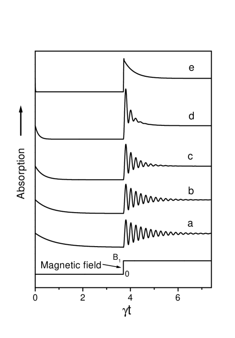
FIG. 6.: Numerically simulated transients for the EIT type transition $F_{g}=1\rightarrow F_{e}=0$ for different optical field intensities. $\Omega^{2}/\Gamma^{2}=2\times 10^{-3}$ (a),  $6\times 10^{-3}$ (b), $0.02$ (c), $0.06$ (d), $2$ (e) ($\Delta=0$, $\gamma=0.002\Gamma$, $\beta_{g}B_{1}=0.03\hbar\Gamma$).

The solution ${\bf y}(t)$ of Eq. 4 was numerically calculated for a magnetic field periodically alternating between two constant values $B_{0}=0$ and $B_{1}\neq 0$. The optical field was taken linearly polarized in the direction perpendicular to the magnetic field. The results are presented in Fig. 6 and 7 for different values of $\Omega/\Gamma$ and $\Delta=0$, $\gamma=0.002\Gamma$ and $\beta_{g}B_{1}=0.03\hbar\Gamma$. For small values of $\Omega/\Gamma$ the $B=0$ and $B\neq 0$ transients show decay times of the order of $\gamma$ for both transitions. The behavior is rather different at larger intensities where the ($B\neq 0$) transient is of comparable duration to the $B=0$ transient for the EIA type transition but is much slower for the EIT type transition. In the latter case, the $B\neq 0$ transient clearly deviates from a simple sine-damped evolution and approaches a pure exponential decay in the large intensity limit with a characteristic rate of the order of $\gamma$.

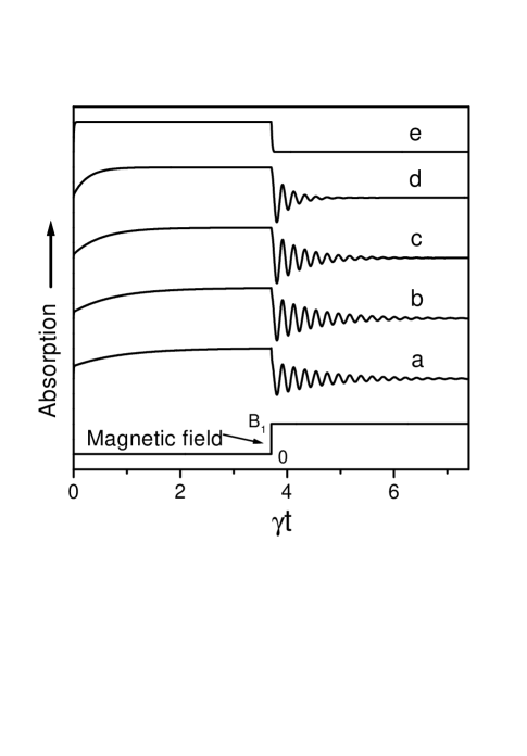
FIG. 7.: Numerically simulated transients for the EIA type transition $F_{g}=1\rightarrow F_{e}=2$ for different optical field intensities. $\Omega^{2}/\Gamma^{2}=2\times 10^{-3}$ (a),  $6\times 10^{-3}$ (b), $0.02$ (c), $0.06$ (d), $2$ (e) ($\Delta=0$, $\gamma=0.002\Gamma$, $\beta_{g}B_{1}=0.03\hbar\Gamma$).

A deeper insight into the transient evolution of these systems can be obtained by the analysis of the eigenvalues $\lambda_{i}$ and eigenvectors ${\bf v}_{i}$ of matrix $M$ which can be numerically calculated ($i=1,\ldots,n$ with $n=16$ and $n=64$ for the considered EIT and EIA transitions respectively). All the real parts of the $\lambda_{i}$’s are negative as expected for a stable system. For $B=0$ all the $\lambda_{i}$’s are real indicating that the equilibrium will be reached through exponential decays. For $B\neq 0$ some of the $\lambda_{i}$’s are complex indicating an oscillating behavior as experimentally observed. For small values of $\Omega/\Gamma$, the $\lambda_{i}$’s can be separated in three groups depending on whether the corresponding absolute values of their real parts are of the order of $\gamma$ or approaches $\Gamma/2$  or $\Gamma$. Group $1$ of eigenvalues, which is the one of interest in this paper, is associated to the evolution of the ground state coherences and populations, groups $2$ and $3$ are related to the relaxation of the optical coherence and excited state populations respectively.

In general, the leading eigenvalue dominating the temporal evolution of the atomic response should be the smallest (observable) one. Since the evolution matrix $M$ includes the escape of the atoms from the interaction region (at rate $\gamma$) it is quite obvious that no $\left|\lambda_{i}\right|$ can be smaller than $\gamma$. As a matter of fact, a constant eigenvalue $\lambda_{1}\equiv-\gamma$ is always present. However, as will be discussed next, the corresponding decay mode is unobservable. In any case, in the limit of low driving field intensity, the leading eigenvalues approach the time-of-flight decay constant $\gamma$ as expected.

The general solution of Eq. 4 is given by:

$${\bf y}(t)=\sum_{i}a_{i}{\bf v}_{i}exp(\lambda_{i}t)-M^{-1}{\bf p}_{0}$$ (5)

where the coefficients $a_{i}$ depend on the initial state of the system. Two conditions are required on a given decay mode to be observable: $a)$ The corresponding eigenvector ${\bf v}_{i}$ must be present in the decomposition (5) of ${\bf y}(t)$ (i.e. $a_{i}\neq 0$). $b)$ The density matrix $\sigma_{i}$ associated to eigenvector ${\bf v}_{i}$ should correspond to a nonzero absorption of the incident optical field.

Using as initial conditions the steady state solutions of Eq. 4 corresponding to $B=0$ or $B=B_{1}$, we have identified the observable decay modes verifying condition $a)$ . The condition $b)$ can be checked by calculating the absorption corresponding to $\sigma_{i}$ according to Eq. 3.

Figs. 8 shows the eigenvalues, corresponding to group $1$, of the observable decay modes as a function of the optical field intensity for the two transitions considered. The decay mode corresponding to $\lambda_{1}\equiv-\gamma$ is unobservable since the corresponding decay is exactly compensated by the pumping term ${\bf p}_{0}$ describing arrival of fresh atoms.

Let us now discuss in more detail the $F_{g}=1\rightarrow F_{e}=0$ transition. This discussion can be simplified by noticing that this system is totally equivalent to the open $\Lambda$ system formed by states $\left|F_{g}=1,m=-1\right\rangle$, $\left|F_{e}=0,m=0\right\rangle$ and $\left|F_{g}=1,m=1\right\rangle$ which can “leak” through spontaneous emission into the “sink” state $\left|F_{g}=0,m=0\right\rangle$. This open $\Lambda$ system has been studied in detail by Renzoni and coworkers [24]. Following their steps, one can write optical Bloch equations for the open $\Lambda$ system incorporating the time-of-flight relaxation constant $\gamma$ for all levels. Analytical expressions of the eigenvalues $\lambda_{i}^{\prime}$ of the corresponding linear differential equations system can be obtained for $B=0$  as a function of the relaxation rates, the Rabi frequency $\Omega$ and the branching ratio $\alpha$ to the sink state. One can check that the observable eigenvalue is in this case $\lambda_{2}^{\prime}\simeq-\gamma+{\cal O}({\Omega}^{2}/\Gamma^{2})$ in agreement with Fig. 8a. For $B\neq 0$ the $\lambda_{i}^{\prime}$’s have to be evaluated numerically.

Taking $\alpha=1/3$, the open $\Lambda$ system exactly describes the $F_{g}=1\rightarrow F_{e}=0$. The use of the simpler $\Lambda$ system helps to the identification of the eigenmode corresponding to a given $\lambda_{i}^{\prime}$. For $B=0$ independently of the optical field intensity, the smallest eigenvalue is $\lambda_{1}^{\prime}\equiv-\gamma$. The corresponding eigenmode is, as expected, the dark state: $\left|\psi_{D}\right\rangle=\sqrt{1/2}\left(\left|F_{g}=1,m=-1\right\rangle-\left|F_{g}=1,m=1\right\rangle\right)$. Since the dark state is not coupled to the light, it’s transient temporal evolution is unobservable. This is not longer the case for $B\neq 0$ since then the dark state is not stationary and consequently the eigenmode corresponding to $\lambda_{1}^{\prime}\sim-\gamma$ is contaminated with the bright state $\left|\psi_{B}\right\rangle=\sqrt{1/2}\left(\left|F_{g}=1,m=-1\right\rangle+\left|F_{g}=1,m=1\right\rangle\right)$ and thus coupled to the excited state. As a consequence the transient evolution corresponding to $\lambda_{1}^{\prime}\sim-\gamma$ becomes observable. It remains the leading eigenvalue even at large values of the driving field intensity. This, together with the fact that the oscillating mode decays at rate $\mathop{\rm Re}\lambda_{3}^{\prime}$ with $\left|\mathop{\rm Re}\lambda_{3}^{\prime}\right|>\left|\lambda_{1}^{\prime}\right|$ (see Fig. 8a) explains the slow exponential component of the $B\neq 0$ transient obtained for large optical field intensity in the EIT type transition (Fig. 6). The dependence on driving field intensity of$\ \lambda_{1}^{\prime}$ presents a minimum at intensity $I_{c}$ ($\Omega^{2}/\Gamma^{2}\simeq 0.1$ in Fig. 8a). Below this critical value, the driving field intensity is responsible for the faster damping of the transient. Above $I_{c}$ an increase in light intensity results in the slowing of the atomic evolution.

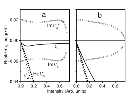
FIG. 8.: Calculated values of the (group 1) observable eigenvalues of the evolution matrix $M$ as a function of light intensity. a) EIT type transition $F_{g}=1\rightarrow F_{e}=0$. b) EIA type transition $F_{g}=1\rightarrow F_{e}=2$. The dashed lines represent real eigenvalues corresponding to the $B=0$ transients. Solid lines represent real eigenvalues of the $B\neq 0$  transients. Circles represent complex eigenvalues ( solid: real part, hollow: imaginary part) of the $B\neq 0$  transients. In (a) the intensity units correspond to the $\Omega^{2}/\Gamma^{2}$ ratio. An increase by a factor $2.5$ of $\left\langle g\|\vec{D}\|e\right\rangle^{2}$ was assumed in (b).

The situation is rather different for the EIA type transition $F_{g}=1\rightarrow F_{e}=2$ (Fig. 8b). In this case, all observable decay modes correspond to eigenvalues whose real parts are (in absolute value) increasing functions of the driving field intensity. As a consequence, there is no exponential decay surviving significantly longer than the damped oscillation for $B\neq 0$.

The simple model calculation presented above explains the main features of the experimental observations. This is somehow surprising in view of the several simplifications of the model with respect to the actual experimental conditions. A first simplification is the neglecting of the atomic motion. It is justified by the fact that the Raman resonance condition between ground state Zeeman sublevels is unaffected by the Doppler effect. In addition, the model does not account for the effect of the optical intensity distribution in the beam profile and of the light propagation across the sample. The influence of the former effect is minimized in the experiments by only collecting light from the central (uniform intensity) portion of the light beam. No significant variation of the transients with the atomic density (optical thickness) of the sample was observed.

We discuss now the role of the contribution of the different hyperfine transitions to the observed transients. The hyperfine structure of the ground level of Rb is well separated in the absorption spectrum. However, due to the Doppler broadening the excited state hyperfine structure is unresolved. Consequently, for a given frequency position of the driving field coupled to one of the ground state hyperfine levels $5S_{1/2}\left(F_{g}\right)$, the atomic response is due to three different transitions to excited state hyperfine levels $5P_{3/2}\left(F_{e}=F_{g},F_{g}\pm 1\right)$. The contribution of each hyperfine transition on the total absorption signal is a function of the specific isotope and transition considered, the precise position of the optical frequency within the Doppler absorption profile and the light intensity. Nevertheless, it was shown that the total absorption presents EIT type coherence resonances when the lower ground state hyperfine level is excited and EIA type resonances for the case of the upper ground state hyperfine level [14, 26, 27]. In the case of the lower ground state level, this is due to the fact that all three hyperfine transitions give rise to EIT [14]. In the case of the upper ground state hyperfine level, the atomic response is quantitatively dominated by the closed transition [$5S_{1/2}\left(F_{g}=2\right)\rightarrow 5P_{3/2}\left(F_{e}=3\right)$ for ⁸⁷Rb] which corresponds to EIA. However this is only true provided that the exciting laser is not too far detuned to the red side of the Doppler absorption profile and that the Rabi frequency remains small in comparison with the excited state hyperfine structure. In fact, significant distortions in the transients were observed for the EIA type transition at maximum available light intensity (not presented). Finally let us remind that for simplicity we have theoretically analyzed the model EIA type transition $F_{g}=1\rightarrow F_{e}=2$. However, we have checked that qualitatively similar results are obtained for the transition $F_{g}=2\rightarrow F_{e}=3$ occurring in ⁸⁷Rb. The good agreement obtained between the observations and the prediction of the simplified model, where a single atomic transition is considered, suggests that the essential features of the atomic response are a direct consequence of the type of the dominant transition(s) rather than the specific transition(s) involved.

The most intriguing result presented above is the unexpected an rather counterintuitive long transient observed for $B\neq 0$ with driving field intensities near saturation for the EIT type resonances. Instead of being the cause of the rapid damping of the atomic evolution, the applied driving field is, in this case, responsible for slowing down the evolution. This is the consequence of the Zeno effect[33] in the sense recently discussed by Luis[34]. In this context, the optical field is seen as a continuous measurement projecting the state of the system onto the DS and thus preventing its evolution. Also, increasing the driving field intensity results in an enhanced stability of the initial quantum state. Following the analysis of Luis, the present result can be seen as the preparation of a specific quantum state (the DS in our case) and its preservation via the Zeno effect. Indeed, a transient such as the one presented in Fig. 6e correspond to a slow non-oscillating evolution of the population in the DS. As Fig. 8a indicates, the survival time of the DS increases once the driving field intensity is above $I_{c}$. Although the quantum Zeno effect is usually presented in terms of the projection postulate associated to measurement in quantum mechanics, such picture is not essential in our case where the whole dynamics is well reproduced by the Bloch equation treatment[35, 34]. The preservation of trapping states in optical pumping experiments at large optical intensities was first reported in [36]. More recently, a similar slowing down of the atomic evolution was discussed and observed by Godun et al. [32].

From a similar perspective, the rather different temporal evolution observed for Hanle/EIA resonances with $B\neq 0$, can be immediately explained by the non existence of a state uncoupled to the light field onto which the system could be projected. As a consequence, the observed and calculated decay rates are increasing functions of the optical intensity.

IV Conclusions.

The transient evolution of the atomic absorption of a linearly polarized optical field as the longitudinal magnetic field is suddenly switched on or off has been observed in Rb vapor. Different transients have been observed depending on the corresponding coherence (Hanle) resonance being of the EIT or EIA type. The main features of the experimentally observed transients are well reproduced by a theoretical model based on the numerical integration of optical Bloch equations where the Zeeman degeneracy of the atomic levels is fully taken into account. As expected, for low driving field intensities all transient evolutions are governed by the time-of-flight relaxation rate. The falling into the DS or the EAS ($B=0$ transients) occurring for EIT and EIA type transitions respectively, happens with similar decay rates that are increasing functions of the driving field intensity. Interesting differences arise between the $B\neq 0$ transients corresponding to the departure from the DS or the EAS for driving field intensities approaching saturation. While the EIA transient is rapidly shortened with the increase of the driving field intensity, the EIT transient shows a slow non oscillating component whose decay time is quite insensitive to the optical field intensity. The latter result is interpreted as the preservation of the initial quantum state via the Zeno effect.

V Acknowledgments.

The authors are thankful to S. Barreiro for his collaboration in the initial stages of the experiment and to J. Fernandez and A. Saez for technical assistance. This work was supported by the Uruguayan agencies: CONICYT, CSIC and PEDECIBA.

REFERENCES

- [1] M.O. Scully, Phys. Reports, 219, 191 (1992).
- [2] For a general overview of coherent processes see M.O. Scully and M.S. Zubairy, Quantum Optics, Cambridge University Press, Cambridge (1997) and references therein.
- [3] G. Alzetta, A. Gozzini, L. Moi and G. Orriols, Nuovo Cimento B 36, 5 (1976).
- [4] E.Arimondo, Coherent population trapping, Progress in Optics XXXV, 257 (1996).
- [5] A. Aspect, E. Arimondo, R. Kaiser, N. Vansteenkiste and C. Cohen-Tannoudji, Phys. Rev. Lett. 61, 826 (1989).
- [6] see S. E. Harris, Physics Today, 50(7) 36 (1997) and references therein.
- [7] S.E. Harris, J.E. Field and A. Imamoğlu, Phys. Rev. Lett. 64, 1107 (1990).
- [8] A.J. Merriam, S.J. Sharpe, M. Shverdin, D. Manuszak, G.Y. Yin and S.E. Harris, Phys. Rev. Lett, 84, 5308 (2000).
- [9] M.O. Scully and M. Fleishhauer, Phys. Rev. Lett. 69, 1360 (1992). H. Lee, M. Fleishhauer and M.O. Scully, Phys. Rev. A 58, 2587 (1998).
- [10] A. Nagel et al, Europhys. Lett. 44, 31 (1998), 48, 385 (1999).
- [11] L.V. Hau, S.E. Harris, Z. Dutton and C.H. Behroozi, Nature 397, 594 (1999).
- [12] M.M. Kash et al, Phys. Rev. Lett. 82, 5229 (1999).
- [13] A.M. Akulshin, S. Barreiro and A. Lezama, Phys. Rev. A 57, 2996 (1998).
- [14] A. Lezama, S. Barreiro and A.M. Akulshin, Phys. Rev. A. 59, 4732 (1999).
- [15] A. Akulshin, S. Barreiro and A. Lezama, Phys. Rev. Lett. 83, 4277 (1999).
- [16] A. Lezama, S. Barreiro,. A. Lipsich and A.M. Akulshin, Phys. Rev. A 61, 013801 (2000).
- [17] D.F. Phillips, A. Fleischhauer, A. Mair, R.L. Walsworth and M.D. Lukin, Phys. Rev. Lett. 86, 783 (2001).
- [18] W. Hanle, Z. Phys. 30, 93 (1924).
- [19] A. Kastler in Nuclear Insturments and Methods 110, 259, North Holland. Amsterdam (1973).
- [20] A. Corney, Atomic and Laser Spectroscopy, Oxford University press (1977).
- [21] W. Happer, Rev. Mod. Phys. 44, 169 (1972) and references therein.
- [22] F. Renzoni, W. Maichen, L. Windholz and E. Arimondo, Phys. Rev. A 55, 3710 (1997).
- [23] F. Renzoni and E. Arimondo, Phys. Rev. A 58, 4717 (1998).
- [24] F. Renzoni, A. Lindner and E. Arimondo, Phys. Rev. A 60, 450 (1999).
- [25] F. Renzoni and E. Arimondo, Opt. Commun. 178, 345 (2000).
- [26] Y. Dancheva, G. Alzetta, S. Cartaleva, M. Taslakov and Ch. Andreeva, Opt. Commun. 178, 103 (2000).
- [27] F. Renzoni, C. Zimmermann, P. Verkerk and E. Arimondo, J. Opt. B: Quantum and Semiclass. Opt. 3, S7 (2001).
- [28] Yong-qing Li and Min Xiao, Opt. Lett. 20, 1489 (1995).
- [29] H.X. Chen, A.V. Durrant, J.P. Marangos and J.A. Vaccaro, Phys. Rev. A, 58, 1545 (1998).
- [30] I.V. Jyotsna and G.S. Agarwal, Phys. Rev. A 52, 3147 (1995).
- [31] E. Arimondo, Phys. Rev. A 54, 2216 (1996).
- [32] R.M. Godun, M.B. d’Arcy, M.K. Oberthaler, G.S. Summy, K. Burnett, Opt. Commun. 169, 301 (1999).
- [33] W.M. Itano, D.J. Heinzen, J.J. Bollinger and D.J. Wineland, Phys. Rev. A 41, 2295 (1990).
- [34] A. Luis, Phys. Rev. A 63, 052112 (2001).
- [35] A. Beige and G.C. Hegerfeldt, Phys. Rev. A 53, 53 (1996).
- [36] S. Slijkhuis, G. Nienhuis and R. Morgenstern, Phys. Rev. A 33, 3977 (1986).