A Novel Approach to Quantum Heuristics for Structured Database Search

Abstract

An algorithm for structured database searching is presented and used to solve the set partition problem. $O(n)$ oracle calls are required in order to obtain a solution, but the probability that this solution is optimal decreases exponentially with problem size. Each oracle call is followed by a measurement, implying that it is necessary to maintain quantum coherence for only one oracle call at a time.

1 Introduction

Quantum computers [1] are thought to be able to solve some problems more efficiently than classical computers. The most important quantum algorithm is the Grover search [2, 3] because of its applicability to solving important computational problems, such as NP-complete problems. In fact, it has already been shown that a nested Grover search can be used to solve the graph-coloring problem, which is NP-complete [4].

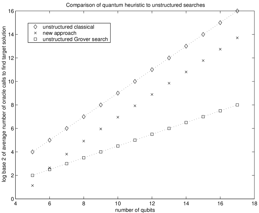
Figure 3: Comparison between number of oracle calls for random classical search ($2^{n-1}$), new algorithm (from simulation and equation 26), and unstructured Grover search ($2^{\frac{n-1}{2}}$). Simulation data is average of 100 problem instances at each value of $n$ from 5 to 15 qubits, 50 instances at 16 qubits, and 40 instances at 17 qubits. Instead of tracking one problem instance from beginning to end, average probability of successful reduction from $n$ to $n-1$ variables is empirically calculated and plugged into equation (26).

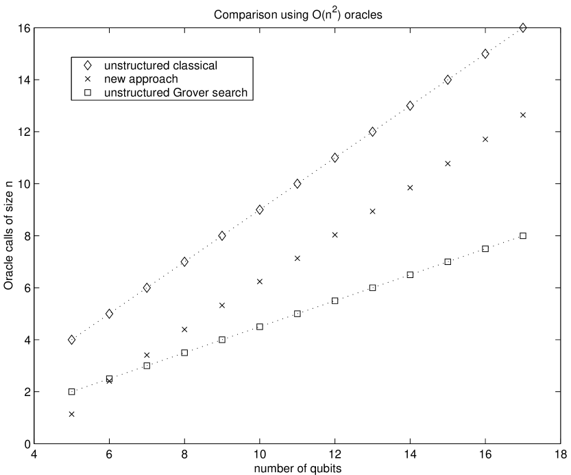
Figure 4: Although the data presented in figure 3 is accurate in terms of the actual number of oracle calls, this algorithm evaluates most of those oracle calls on only a subset of the original variables. Taking, for example, an oracle that has complexity $O(n^{2})$, we can adjust the data of the new approach by weighing the oracle calls by how many variables they operate on. This shows a noticeable improvement.

Here I report a new approach to structured database search, and I apply it to the set partition problem, which is NP-complete. Through simulation, I find in this application that the number of required oracle calls is fewer than a random classical search, but more than an unstructred Grover search (see figures 3 and 4). However, it is only necessary to maintain quantum coherence for a single oracle call at a time, unlike Grover searches which require that quantum coherence is maintained throughout the entire running time. Since the short coherence times of quantum systems is the biggest obstacle to quantum computing [5], this is an interesting result.

I will start by presenting the general principles outlining the new approach to structured database search. I will then show how they can be specifically applied to the set partition problem.

2 Quantum Algorithm for Structured Database Search

2.1 Definitions of Quantum Operators

In order to search a mathematically-specified database, our quantum computer will need two registers. One is for the index of the database item ($n$ qubits) and the other is for the data associated with that index (size requirements discussed later). This is a mathematically-specified database because the data associated with the index is the result of a mathematical function when given the index as input.

The first operator to define is one that creates the database to be searched without making any measurement on the system. The most natural way to accomplish this is in a two-step process. First,

$$\hat{W}_{s}\equiv\hat{W}\otimes\hat{I}$$ (1)

or equivalently,

$$\hat{W}_{s}|i\rangle|j\rangle\equiv(\hat{W}|i\rangle)|j\rangle$$ (2)

where $\hat{W}$ is an $n$-bit Walsh-Hadamard transform [6].
Second, if we take $P$ to be the mathematical function relating the index of the database item to its data, we want to define a unitary operator that implements this function:

$$\hat{P}|i\rangle|j\rangle\equiv|i\rangle|(j+P(i))modN\rangle$$ (3)

where $modN$ allows for overflow in the second register ($N\neq 2^{n}$). In an optimization problem, $P$ is a cost function. Now, if we define

$$\hat{A}\equiv\hat{P}\cdot\hat{W}_{s}$$ (4)

we have that

$$\hat{A}|i\rangle|j\rangle=\frac{1}{2^{\frac{n}{2}}}\sum_{k=0}^{2^{n}-1}(-1)^{i\oplus k}|k\rangle|(j+P(k))modN\rangle$$ (5)

where $\oplus$ is binary bit-wise addition. These definitions imply that

$$\hat{A}^{-1}=\hat{W}_{s}^{-1}\cdot\hat{P}^{-1}=\hat{W}_{s}\cdot\hat{P}^{-1}$$ (6)

where

$$\hat{P}^{-1}|i\rangle|j\rangle\equiv|i\rangle|(j+N-P(i))modN\rangle$$ (7)

From this we see that

$$\hat{A}^{-1}|i\rangle|j\rangle=\frac{1}{2^{\frac{n}{2}}}(\sum_{k=0}^{2^{n}-1}(-1)^{i\oplus k}|k\rangle)|(j+N-P(i))modN\rangle$$ (8)

Most importantly,

$$\hat{A}|0\rangle|0\rangle=\frac{1}{2^{\frac{n}{2}}}\sum_{s=0}^{2^{n}-1}|s\rangle|P(s)\rangle$$ (9)

The following phase flip operator will also be needed:

$$\hat{S}_{\epsilon}^{\pi}|i\rangle|j\rangle\equiv\left\{\begin{array}[]{ll}-|i\rangle|j\rangle&j\leq\epsilon\\ \;\;\,|i\rangle|j\rangle&j>\epsilon\end{array}\right.$$ (12)

States $i$ for which $P(i)$ is less than or equal to $\epsilon$ are called good, and states $i$ for which $P(i)$ is greater than epsilon are called nogood. In general, our target state will be any $i_{0}$, for which $P(i_{0})$ is a global minimum.
Finally,

$$\hat{D}\equiv\hat{A}^{-1}\cdot\hat{S}_{\epsilon}^{\pi}\cdot\hat{A}$$ (13)

You may notice that $\hat{D}$ is actually part of the general Grover operator [7], but the use here will be very intuitively different, as I will discuss later.

2.2 Implementation of Quantum Operators

In order to use these quantum operators in an algorithm, it is necessary to show that they are efficiently implementable. $\hat{W}_{s}$ is trivial. $\hat{P}$ relies only on addition and a function evalution of $P$. Since these are both efficient classically, they can be implemented efficiently on a quantum computer [1]. $\hat{S}_{\epsilon}^{\pi}$ can be implemented with the use of a single work bit. First, add $(N-\epsilon)$ to the second register and store overflow in the work bit. Second, invert the work bit and perform a conditional phase flip. Finally, uncompute to clear the work bit.

2.3 The Algorithm

Here I will present the steps of an algorithm for structured database search, then proceed to fill in the missing details.

1) Clear to $|0\rangle|0\rangle$     $|\psi\rangle=|0\rangle|0\rangle$

2) Apply $\hat{D}\qquad\qquad\qquad\;\;\,|\psi\rangle=(|0\rangle-\frac{2}{2^{\frac{n}{2}}}\sum_{good}|s\rangle)|0\rangle$

3) Measure $\qquad\qquad\qquad\;\;\,|\psi\rangle=|m\rangle|0\rangle$

4) Use $m$ to half the size of the database.

5) Repeat steps $1-4$ until a solution is found.

2.4 Using Measurement to Reduce Problem Size

Step 4 of the above algorithm is the crucial step. The idea is basically as follows: $\hat{D}$ consists of three operators: $\hat{A}$ creates a database, $\hat{S}_{\epsilon}^{\pi}$ flips phases of good states, and $\hat{A}^{-1}$ uncomputes. $\hat{S}_{\epsilon}^{\pi}$ flips phases based on the value in the 2nd register, but the subsequent phase interference affects what is measured in the 1st register. Using $|{m}\rangle$, we want to deduce which first register values were entangled to second register values less than $\epsilon$.

2.4.1 Viewpoint as a Quantum Oracle

I have defined $\hat{D}$ as a series of quantum operators on two registers. However, in the context of solving computational problems with quantum algorithms, it is important to understand that $\hat{D}$ can be equivalently viewed as operations on just one quantum register with the help of a ’quantum oracle.’

$$\hat{D} = \hat{A}^{-1}\cdot\hat{S}_{\epsilon}^{\pi}\cdot\hat{A}$$ (14)

$$= \hat{W}_{s}\cdot\hat{P}^{-1}\cdot\hat{S}_{\epsilon}^{\pi}\cdot\hat{P}\cdot\hat{W}_{s}$$

$$= \hat{W}_{s}\cdot\textrm{(quantum oracle)}\cdot\hat{W}_{s}$$

In the first viewpoint, a function evaluation acts in parallel to entangle all possible inputs to their outputs, and a phase operator flips the phases of target states based on their output value. Then, in uncomputation, the inverse function evaluation returns all values in the second register to $|0\rangle$ so that phase interference can occur between different states in the first register.

In the quantum oracle viewpoint, only one quantum register is used explicitly. The phases of certain target states are flipped by a quantum oracle that uses machinery whose details we do not examine.

2.4.2 Deterministic Measurement

So far, the only new idea I have presented is to propose that the steps in section 3 could be considered as an algorithm. The rest of what I have covered is basically a summary of how I understand and use existing ideas. Now I will begin to explain step 4 of the algorithm and justify the claim that $\hat{D}$ can be used for structured database search.

In general, the state $\hat{D}|{0}\rangle|{0}\rangle$ will be a superposition of many eigenstates of the computational basis, and when we measure this state, the value we obtain for $m$ is not deterministic.

However, it is very useful to ask the following question: what would be the structure of a problem instance for which $\hat{D}|{0}\rangle|{0}\rangle$ is an eigenstate of the computational basis? This is an easy question to answer with the quantum oracle viewpoint:

$$\hat{W}\cdot\textrm{(oracle)}\cdot\hat{W}|{0}\rangle = |{x}\rangle$$

$$\Rightarrow\textrm{(oracle)}\cdot\hat{W}|{0}\rangle = \hat{W}|{x}\rangle$$ (15)

$$\textrm{using}\;\;\hat{W}^{2}=\hat{I}$$

From this we see that if the best half of the states in our database exactly corresponds to the half of the database whose phase is flipped in the Walsh-Hadamard transformation of some $|{x}\rangle$, then after measurement we will obtain $|{m}\rangle=|{x}\rangle$ with certainty.

2.4.3 Choosing a Subset

Based on the function $P$, we could divide our database of $2^{n}$ states into a best half and worst half. The 1st register values of the best half will not be random, or else this would be an unstructured database search. Nonetheless, their structure could easily be sufficiently complicated that we could not adjust $\hat{A}$ to create a superposition of only those states [8]. More importantly, if our goal is to reduce the size of our database by a factor of 2, then it is sufficient to choose any half that still contains the state $i_{0}$. Therefore, it seems reasonable to look for a way to approximate the best half of solutions.

I propose the following: after measuring and obtaining $|{m}\rangle$, keep the $2^{n-1}$ items whose phases are flipped in the expansion of $\hat{W}|{m}\rangle$. This will be the half of the database that we use to approximate the best half, motivated by the finding in section 2.4.2 that if this approximate half was really the best half, then we would have measured $|{m}\rangle$ with certainty.

Details for exactly how these states are chosen will be given later in the context of the set partition problem. In this case we will see that it is always possible to efficiently create a superposition of the database items we want, but in general this may or may not be true.

2.4.4 Measurement Probabilities

The above section implicity assumes that we can choose an $\epsilon$ such that $\hat{S}_{\epsilon}^{\pi}$ flips exactly half of the states of the database. However, this is not a strict requirement.

When measuring the state $\hat{D}|0\rangle|0\rangle$, what is the probability of measuring a given state $|x\rangle$ in the first register? (second register is deterministically $|0\rangle$)

First, in order to help quantify the action of the oracle, define:

$$\Theta_{\epsilon}(k)\equiv\left\{\begin{array}[]{ll}-1&P(k)\leq\epsilon\\ \;\;\,1&P(k)>\epsilon\end{array}\right.$$ (18)

Now we can calculate the probability of measuring $|x\rangle$, $M(x)$:

$$M(x) \equiv \arrowvert\langle x|\hat{D}|0\rangle\arrowvert^{2}$$ (19)

$$\langle x|\hat{D}|0\rangle = \langle x|\hat{W}\cdot\textrm{oracle}\cdot\hat{W}|0\rangle$$ (20)

$$= \Big{(}\frac{1}{2^{\frac{n}{2}}}\sum_{k}\langle k|(-1)^{k\oplus x}\Big{)}\Big{(}\frac{1}{2^{\frac{n}{2}}}\sum_{k}\Theta_{\epsilon}(k)|k\rangle\Big{)}$$

$$= \frac{1}{2^{n}}\sum_{k}(-1)^{k\oplus x}\Theta_{\epsilon}(k)$$

Now, let

F = number of states $|k\rangle$ such that $(-1)^{k\oplus x}=-1$ and $\Theta_{\epsilon}(k)=-1$

and

N = number of states $|k\rangle$ such that $(-1)^{k\oplus x}=1$ and $\Theta_{\epsilon}(k)=-1$

With a little algebra,

$$\langle x|\hat{D}|0\rangle=\frac{F-N}{2^{n-1}}$$ (21)

$$\Rightarrow M(x)=\Big{(}\frac{F-N}{2^{n-1}}\Big{)}^{2}$$ (22)

3 Application to the Set Partition Problem

3.1 Statement of Problem

Given a set $S=\{a_{1},a_{2},\ldots,a_{n}\}$ of positive numbers, find a subset $s\subset S$ such that $P$ is minimized, where

$$P(s)=\Big{|}\sum_{a_{j}\in s}a_{j}-\sum_{a_{k}\notin s}a_{k}\Big{|}$$ (23)

Not only is this problem at the heart of NP-completeness [9], but it is framed in the manner of a binary optimization that minimizes a cost function. While the nested Grover search is the best result so far for solving NP-complete problems, it relies on a structure that does not exist in optimizations.

3.2 Solving Set Partition

3.2.1 Using the Algorithm

The function $P$ in (23) takes the place of the function $P$ used in (3). The first register of our quantum computer will still be $n$ qubits. If each of the numbers in the set $S$ has $b$ bits of precision, then the second quantum register will have to be $\lceil b+\log{n}\rceil$ qubits in order to accomodate the largest possible value of $P(s)$, which is $N=n2^{b}$. If $b$ is large, this requirement can be significantly relaxed. The only strict requirement is that $\hat{S}_{\epsilon}^{\pi}$ has to distinguish between goods and nogoods.

The registers also are set-up such that each qubit $i$ in the 1st register corresponds to a specific $a_{i}$ in $S$ ($\Rightarrow$ $P(s)=\sum(-1)^{i}a_{i}$). The set partition problem has a degeneracy because $P(s)$ is the absolute value of a difference, so in solving this problem with a quantum algorithm I only consider a database of solutions where the smallest number is in the subset $s$. In principle, however, any $a_{i}$ could be used for this purpose. Also, this problem becomes deterministic at $n=4$, so I only solve cases $n\geq 5$.

Most importantly, I need to specify exactly how to reduce the size of the database. Suppose that the state $|{m}\rangle$ that we measure has $l$ 1’s in its binary representation. This means that there are $n-l$ $a_{i}s$ in the subset $s$ and $l$ $a_{i}s$ not in $s$. The procedure is as follows: if $l$ is even, then choose the smallest $a_{i}$ and call it $t$. In $S$, replace each $a_{i}$ not in $s$ with the difference $a_{i}-t$ and remove $t$ from $S$. If $l$ is odd, then add $a_{1}$ to the group of $a_{i}^{\prime}s$ not in $s$ and use the same procedure. In order to solve a problem instance, $n-4$ of these decisions must be made, and with classical processing they can tracked to give a solution of $n$ variables at the end of the iterations.

3.2.2 Simulations

My wish is not to submit these simulations as primary evidence that my method works for solving NP-complete and optimization problems. Rather, the above sections contain enough information to see that this will be true, and I will discuss some of these points in section 4. However, the complexity of this solution cannot be predicted analytically, so a simulation helps to quantify a few examples of using this algorithm.

The simulations were set-up as follows: a random instance of the problem was generated, and the probability of measuring each state was calculated using (21). Each possible measurement was tagged good or bad based on whether it would led to inclusion of the $i_{0}$ after database reduction. For a given iteration on a specific problem instance, these probabilities can be summed to obtain the total probability of making either a good or bad measurement. When these probabilities are averaged over many problem instances they are denoted $p_{G}$ and $p_{B}$ respectively.

Given average values of $p_{G}$ and $p_{B}$ for runs with 5 qubits up to $n$ qubits, the complexity in terms of number of oracle calls can be calculated as follows:

The probability of finding the correct solution in a given run:

$$P_{c}=\Pi_{i=5}^{n}p_{G}(i)$$ (24)

The algorithm will produce a solution after $n$ iterations. However, if we choose to only use certain types of states for measurement, multiple oracle calls may be required for a given iteration. The average number of oracle calls for a run is:

$$N_{0}=\sum_{i=5}^{n}\frac{1}{p_{G}(i)+p_{B}(i)}$$ (25)

In order for the correct solution to be found after $r$ runs of the algorithm, an incorrect solution must be found $r-1$ times in a row, followed by a correct solution on the $rth$ try. Therefore, the complexity is given by:

$$Complexity = P_{c}\cdot N_{0}+(1-P_{c})\cdot P_{c}\cdot(2N_{0})+(1-P_{c})^{2}\cdot P_{c}\cdot(3N_{0})+\ldots$$

$$= N_{0}P_{c}\sum_{k=1}^{\infty}k(1-P_{c})^{k-1}$$

$$Complexity =$$

$$\Big{(}\sum_{i=5}^{n}\frac{1}{p_{G}(i)+p_{B}(i)}\Big{)}\Big{(}\Pi_{i=5}^{n}p_{G}(i)\Big{)}\Big{(}\sum_{k=1}^{\infty}k(1-(\Pi_{i=5}^{n}p_{G}(i)))^{k-1}\Big{)}$$ (26)

A few comments:
1) The form of $P_{c}$ implies that this complexity will grow exponentially unless $p_{G}\to 1$ as $n\to\infty$.
2) In calculating the infinite sum from simulation data, I just add terms until they are below the threshold $10^{-4}$. I checked this against smaller thresholds and it does not appear to affect results.
3) The asymptotic value of the exponential part of the complexity can be estimated by $O((\frac{1}{p_{G}(i)})^{n})$ using the largest $i$ for which $p_{G}$ is known, but this will not necessarily give the whole picture.

3.2.3 Results of Simulation

At each iteration, an $n$ variable problem is reduced to an $n-1$ variable problem, thus reducing the size of the database by a factor of 2. If the target solution remains in the database, then this was a successful reduction. Figure 1 shows the average probability of a successful database reduction at various problem sizes. The first measurement scheme repeats the first three steps of section 2.3 until $|{m}\rangle=|{2^{k}+2^{j}}\rangle$. The second scheme uses any $|{m}\rangle\neq|{0}\rangle$ as a valid measurement. As figure 1 clearly indicates, the first scheme is more successful. Based on the form of (26), improving $p_{G}$ can save an exponential number of steps, so the first scheme is adopted in future simulations.

In these first two simulations, the $\epsilon$ appearing in (12) and (18) was not explicity used. In order to test an ideal case, I cheated and flipped the phase of exactly half of the states in the database. However, it was shown in (21) that this is not necessary. In order to obtain realistic complexity data, I henceforth simulate the algorithm using a naiive method that flips all states whose cost is below $.29\sum_{i}a_{i}$. In general, if we know what fraction of states we want to flip, better methods than the naiive one I employ are available using the density of states for the partition problem [10].

As stated in section 2.3, the algorithm requires $n$ iterations to find a solution. However, if the $l=2$ measurement scheme is employed, some measurements will be thrown out, in which case extra oracle calls must be made. Figure 2 is a plot of data for (25) with a linear fit. This shows that we have paid a small price by using the $l=2$ measurement scheme: instead of taking $n$ iterations to get a solution we need $O(n)$.

The asymptotic behavior of the algorithm is related to the asymptotic behavior of figure 1. It is possible that as $n\rightarrow\infty$, $p_{G}(n)\rightarrow.5$, which is equivalent to a random decision (there is no reason to expect $p_{G}$ would go lower than .5). In this case, the asymptotic behavior would be no better than a classical search. If the asymptotic behavior of $p_{G}\geq.5$, then of course we are in luck. Of course, this cannot be determined from simulation. But by examining figure 1 I argue that if $p_{G}$ falls off slowly enough, then we still benefit.

Figure 3 is a comparison between three different searches. A random classical search will, on average, find a solution after $2^{n-1}$ tries. The data for this algorithm is based on simulations using the naiive phase-flipping scheme described above and plugged into 26. An unstructured Grover search requires $2^{\frac{n-1}{2}}$ oracle calls (rotates towards 2 target solutions). Comparisons to classical search and further comments are given in section 4.

However, the data in figure 3 slightly misrepresents the new approach, because although each iteration of the algorithm makes at least one oracle call, these oracle calls use fewer than $n$ variables. For example, assume for a moment that the oracle function takes $O(n^{2})$ steps to implement. When the algorithm makes an oracle call on $n-3$ variables, let us count that as only $(\frac{n-3}{n})^{2}$ of a call, because both the classical and Grover unstructured searches always make oracle calls using all $n$ variables. Figure 4 shows data adjusted in this manner, and it shows a noticeable improvement.

4 Comments on this Algorithm

Since this is a new method, it may be necessary to explain the intuition behind how it works.

4.1 Summary of Results

The algorithm presented in section 2.3 can be used in order to perform structured database search. It returns a solution after $O(n)$ oracle calls, but (26) shows that the probability of this being an optimal solution decreases exponentially. Each oracle call is followed by a measurement, implying that quantum coherence is necessary for only one oracle call at a time.

4.2 A Quantum Heuristic

4.2.1 Description of the Heuristic

We have a database of size $2^{n}$. Each of the $2^{n}-1$ possible states that could be measured in step 4 of the algorithm implies a subspace with $2^{n-1}$ members (see section 2.4.3). We are most likely to explore a given subspace if the number of good states included in that subspace and number of good states not included in that subspace differ (see equation (21)).

4.2.2 Meaning of Heuristic in $l=2$ example

In solving the set partition problem, measurements of the form $|{2^{k}+2^{j}}\rangle$ have the simple interpretation that the database is reduced by placing two numbers from the set $S$ in different groups. If placing two numbers in different groups results in a large number of either low-lying or non-low-lying solutions , then the probability of following this path is high. In fact, the data in figure 2 implies that in the set partition problem, states of the form $|{2^{k}+2^{j}}\rangle|{0}\rangle$ are peaked in $\hat{D}|{0}\rangle|{0}\rangle$ The fact that $p_{G}$ is greater than .5 (as can be seen in figure 1) means that a subspace with a non-random distrubtion of low-lying states has a better than $50\%$ chance of containing target solution.

4.2.3 Quantum Heuristic vs. Classical Heuristic

Differencing heuristics already exist to solve partition problems classically [11, 12]. The quantum heuristic is different because it can take into account properties of a whole database for a specific problem instance. For example, putting the largest two numbers into different sets is a good classical heuristic because it works well on most problem instances. However, the probability of putting the two largest numbers in different sets in a given run of this algorithm is based on how many low-lying solutions that action creates in the specific instance being solved.

4.3 This is not Amplitude Amplification

It is important to understand that this approach does not utilize amplitude amplification as used in other algorithms [2, 13, 14]. The states that are peaked in $\hat{D}|{0}\rangle|{0}\rangle$ represent subspaces of the database to be searched on future iterations. They no longer represent the states indexing the database. Furthermore, there is the following difference with amplitude amplification: if a classical algorithm makes $2^{n}$ oracle calls, it will have explicity checked the cost of $2^{n}$ different database items. However, if a Grover search makes $2^{\frac{n}{2}}$ oracle calls to rotate to a target state, at the end it will only have explicitly checked the cost of a single database item because only one measurement occurs. This algorithm falls somewhere in between those two extremes. After every $O(n)$ oracle calls a database item is checked. However, this algorithm is more likely than a classical algorithm to check the same database item multiple times because quantum measurement is probabilistic.

4.4 Usefulness of this Approach

The most important goal is to find a solution as quickly as possible. So far, I have not demonstrated that this algorithm is any better at finding solutions than a Grover search (although it has different properties as noted in section 4.3). Whether or not there are benefits reducing the required coherence time is hard to say. If it becomes more difficult to perform many logic gates as system size increases (see [15] for proposed implementation where this is true), then it is possible to imagine a situation where it is much more feasible to implement this algorithm than a Grover search for certain problem sizes.

As compared to classical algorithms, this approach has interesting properities. It is certainly impossible to solve a problem this way classically. The steps in section 2.3 outline what is probably the simplest approach to using the properties of an entire database to decide how to parse the tree of possible solutions to an optimization problem. It may be that this algorithm’s usefulness would be not be in solving the set partition problem, but in solving problems where little is known about the database structure a riori.

Comments

I would appreciate comments sent to brian34@feynman.stanford.edu.

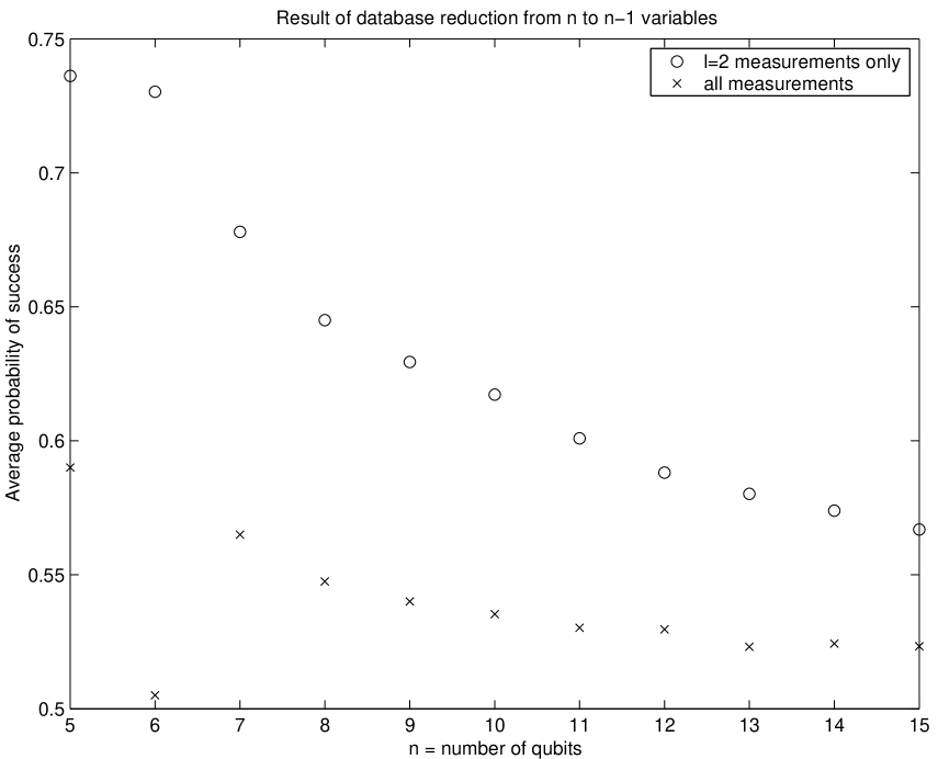
Figure 1: The probability of a correct database reduction from $n$ to $n-1$ variables is shown for two schemes. In one scheme $|{m}\rangle=|{2^{k}+2^{j}}\rangle$ is allowed. In the second, $|{m}\rangle\neq|{0}\rangle$ is allowed. In both simulations, $\hat{S}_{\epsilon}^{\pi}$ is idealized to flip the phase of half of the states in the database. Each data point in the first scheme is the average of 100 problem instances, each data point in the second scheme is the average of 50 instances.

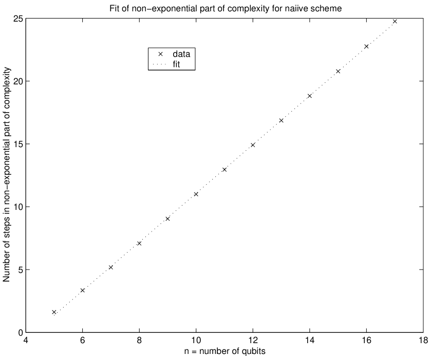
Figure 2: Plot of the number of oracle calls necessary to perform one run of the algorithm for a simulation with $\epsilon=.29\sum_{i}a_{i}$. This data is plotted to quantify the extra runs that are required in order to obtain $l=2$ measurements. The data is fit to $1.9401\cdot(n-4)-.5735$ to show that the number of calls per run is still $O(n)$.

References

- [1] D. Deutsch, “Quantum theory, the Church-Turing principle and the universal quantum computer”, Proc. Roy. Soc. London Ser. A 400, 97-117 (1985)
- [2] L.K. Grover, Phys. Rev. Lett. 79, 325 (1997).
- [3] L.K. Grover, Phys. Rev. Lett. 80, 4329 (1998).
- [4] N.J. Cerf, L.K. Grover, and C.P. Williams, “Nested quantum search and NP-complete problems”, Los Alamos e-print quant-ph/9806078
- [5] F. Yamaguchi, C.P. Master, and Y. Yamamoto, “Concurrent Quantum Computation”, Los-Alamos e-print quant-ph/0005128
- [6] Y. Yamamoto, class notes for Applied Physics 225 “Quantum Information Theory”, Stanford University, http://feynman.stanford.edu/class/ap225/2001/chapter6.pdf.
- [7] G. Brassard, P. Hoyer, and A. Tapp, “Quantum Counting”, Los Alamos e-print quant-ph/9805082
- [8] A. Barenco et al., Phys. Rev. A 52, 3457 (1995).
- [9] M.R. Garey and D.S. Johnson, Computers and Intractibility. A Guide to the Theory of NP-Completeness W.H. Freeman, New York, 1997.
- [10] Personal communication, Vadim Smelyanskiy and Dogan Timuçin
- [11] R. Korf, “Complete anytime algorithm for number partitioning”, Artificial Intelligence, 106 no.2, 181-203 (1998).
- [12] S. Mertens, “A complete anytime algorithm for balanced number partitioning”, Los Alamos e-print cond-mat/9903011
- [13] G. Brassard, P. Hoyer, M. Mosca, A. Tapp, “Amplitude Amplification and Estimation”, Los Alamos e-print quant-ph/0005055
- [14] T. Hogg, “Single-step Quantum Search Using Problem Structure”, Int. J. Mod. Phys. C11 739-774 (2000), Los Alamos e-print quant-ph/9812049
- [15] T.D. Ladd, J.R. Goldman, A. Dâna, F. Yamaguchi, Y. Yamamoto, “Quantum Computation in a One-Dimensional Crystal Lattice with NMR Force Microscopy”, Los Alamos e-print quant-ph/0009122.