A Knob for Changing Light Propagation from Subluminal to Superluminal

Abstract

We show how the application of a coupling field connecting the two lower metastable states of a $\Lambda$-system can produce a variety of new results on the propagation of a weak electromagnetic pulse. In principle the light propagation can be changed from subluminal to superluminal. The negative group index results from the regions of anomalous dispersion and gain in susceptibility.

PACS number(s): 42.50.Gy, 42.25.Bs, 42.25.Kb

A series of experiments have demonstrated both subluminal [1, 2, 3, 4, 5] and superluminal [6, 7, 8] propagation of light in a dispersive medium. The key to these successful demonstration lies in one’s ability to control optical properties of a medium by a laser field. Harris et. al. [9] suggested how the electromagnetically induced transparency (EIT) [10] can be used to obtain group velocities $v_{g}$ [11] much smaller than the velocity of light in vacuum. Early experiments [1, 2] produced values of group index $n_{g}=c/v_{g}$ in the range $10^{2}-10^{3}$. Hau et. al. [3] could reduce the group velocity to 17 meter/sec in a Bose condensate. This was followed by an experiment in Rb vapor demonstrating reduction of group velocity to $90$ meter/sec [4] and to 8 meter/sec [5]. These experiments were based on the fact that EIT not only makes absorption zero at the line center but also leads to a dispersion profile [10, 12] with a sharp derivative near the line center of the absorption line. In a different development Wang et. al. [6] demonstrated superluminal propagation following the work of Chiao and coworkers [13-16; see also 17]. Wang et. al. used basically stimulated Raman effect with the pumping beam replaced by a bichromatic field. This produces two regions of Raman gain with a region in between which has the right anomalous dispersion but with a negligible gain [18, 19]. In this communication we propose a scheme where by changing a knob - an additional coupling field, one can switch the propagation of light from subluminal to superluminal. We basically use the $\Lambda$-system driven by a coherent control field, which has been extensively discussed in connection with subluminal propagation [1, 2, 3, 4, 5]. We apply, in addition, a field (referred to as LL coupling field) on the lower levels of the $\Lambda$-system and demonstrate how the application of the lower level coupling field can produce regions in optical response with appropriate dispersion profile. The dispersion can change from normal to anomalous depending on the intensity of the LL coupling field [20, 21, 22]. In addition, under suitable conditions the amplification of the light remains negligibly small.

We consider the scheme shown in the Fig. 1(a). We consider propagation of light pulse whose central frequency $\omega_{1}$ is close to the frequency of the atomic transition $|1\rangle\leftrightarrow|3\rangle$ . We apply a control field on the optical transition $|1\rangle\leftrightarrow|2\rangle$. The transition $|2\rangle\leftrightarrow|3\rangle$ is generally electric dipole forbidden transition. The states $|2\rangle$ and $|3\rangle$ are metastable states. We apply a field of frequency $\omega_{3}$ on the transition $|2\rangle\leftrightarrow|3\rangle$. The nature of this field will depend on the level structure. It could be a microwave field, say, in case of Na or an infrared field in case of ²⁰⁸Pb. Moreover, it could be a dc field if one is considering transparency with Zeeman sublevels[5]. Let $2G=2\vec{d}_{12}.\vec{E}_{c}/\hbar~{}$ and $~{}2\Omega$ be the Rabi frequencies of the control field $\vec{E}_{c}$ and the LL coupling field, respectively. The state $|1\rangle$ decays to the states $|3\rangle$ and $|2\rangle$ at the rates $2\gamma_{1}$ and $2\gamma_{2}$. For simplicity we ignore all collisional effects though these could be easily included. What is relevant for further consideration is the group velocity $v_{g}$ for the pulse applied on the transition $|1\rangle\leftrightarrow|3\rangle$. The $v_{g}$ is related to the susceptibility $\chi_{{}_{13}}(\omega_{1})$ for transition $|1\rangle\leftrightarrow|3\rangle$

$$v_{g}=\frac{c}{1+2\pi{\chi^{{}^{\prime}}_{{}_{13}}}(\omega_{1})+2\pi\omega_{1}\frac{\partial{\chi^{{}^{\prime}}_{{}_{13}}}(\omega_{1})}{\partial\omega_{1}}}~{}~{},$$ (1)

where ${\chi^{{}^{\prime}}_{{}_{13}}}(\omega_{1})$ is the real part of $\chi_{{}_{13}}(\omega_{1})$. We assume that we are working under condition such that Im$[\chi_{{}_{13}}(\omega_{1})]=\chi^{\prime\prime}_{{}_{13}}(\omega_{1})\approx 0$. The susceptibility $\chi_{{}_{13}}(\omega_{1})$ will depend strongly on the intensities and the frequencies of the control laser and the LL coupling field. We concentrate on the group velocity though actual pulse profiles could be easily simulated [23]. This susceptibility $\chi_{{}_{13}}(\omega_{1})$ is obtained by solving the density matrix equations for the $\Lambda$-system of Fig. 1(a), i.e., by calculating the density matrix element $\rho_{13}$ to first order in the applied optical field on the transition $|1\rangle\leftrightarrow|3\rangle$ but to all orders in the control field and the LL coupling field. By making a unitary transformation from the density matrix $\rho$ to $\sigma$ via

$$\rho_{12}=\sigma_{12}e^{-i\omega_{2}t}~{}~{}~{};~{}~{}~{}\rho_{13}=\sigma_{13}e^{-i(\omega_{2}+\omega_{3})t}~{}~{}~{};~{}~{}~{}\rho_{23}=\sigma_{23}e^{-i\omega_{3}t}~{}~{},$$ (2)

we have the relevant density matrix equations

$$\dot{\sigma}_{11} = iG\sigma_{21}+ige^{-i\Delta_{4}t}\sigma_{31}-iG^{*}\sigma_{12}-ig^{*}e^{i\Delta_{4}t}\sigma_{13}-2(\gamma_{1}+\gamma_{2})\sigma_{11}~{},$$ (3)

$$\dot{\sigma}_{22} = iG^{*}\sigma_{12}+i\Omega\sigma_{32}-iG\sigma_{21}-i\Omega^{*}\sigma_{23}+2\gamma_{2}\sigma_{11}~{},$$ (4)

$$\dot{\sigma}_{12} = -[\gamma_{1}+\gamma_{2}+\Gamma_{12}-i\Delta_{2}]\sigma_{12}+iG\sigma_{22}+ige^{-i\Delta_{4}t}\sigma_{32}-iG\sigma_{11}-i\Omega^{*}\sigma_{13}~{},$$ (5)

$$\dot{\sigma}_{13} = -[\gamma_{1}+\gamma_{2}+\Gamma_{13}-i(\Delta_{2}+\Delta_{3})]\sigma_{13}+iG\sigma_{23}+ige^{-i\Delta_{4}t}\sigma_{33}-ige^{-i\Delta_{4}t}\sigma_{11}-i\Omega\sigma_{12}~{},$$ (6)

$$\dot{\sigma}_{23} = -(\Gamma_{23}-i\Delta_{3})\sigma_{23}+iG^{*}\sigma_{13}+i\Omega\sigma_{33}-ige^{-i\Delta_{4}t}\sigma_{23}-i\Omega\sigma_{22}~{},$$ (7)

where $\Gamma$’s give collisional dephasings, the detunings $\Delta_{1},~{}\Delta_{2},~{}\Delta_{3},~{}\Delta_{4}$ and the coupling constant$~{}g$ are defined by

$$\Delta_{1}=\omega_{1}-\omega_{13}~{};~{}\Delta_{2}=\omega_{2}-\omega_{12}~{};~{}\Delta_{3}=\omega_{3}-\omega_{23}~{};~{}\Delta_{4}=\Delta_{1}-\Delta_{2}-\Delta_{3}~{};~{}g=\frac{\vec{d}_{13}.\vec{E}_{p}}{\hbar}~{}~{}.$$ (8)

The susceptibility $\chi_{{}_{13}}$ can be obtained by considering the steady state solution of (3) to first order in the field on the transition $|1\rangle\leftrightarrow|3\rangle$. For this purpose we write

$$\sigma=\sigma^{0}~{}+~{}\frac{g}{\gamma}~{}e^{-i\Delta_{4}t}~{}\sigma^{+}~{}+~{}\frac{g^{*}}{\gamma}~{}e^{i\Delta_{4}t}~{}\sigma^{-}+......$$ (9)

The $13-$ element of $\sigma^{+}$ will yield the susceptibility at the frequency $\omega_{1}$ as can be seen by combining Eqs. (2) and (5)

$$\chi_{{}_{13}}(\omega_{1})=\frac{N|d_{13}|^{2}}{\hbar\gamma}\sigma_{13}^{+}~{}~{},$$ (10)

where $N$ is the density of atoms. In the above equations we have, for simplicity, set $\gamma_{1}=\gamma_{2}=\gamma$. The group velocity can be obtained by substituting (6) in (1). In presence of the LL coupling field it is difficult to obtain algebraically simple expressions for $\chi_{{}_{13}}$. However Eqs. (3) can be solved numerically. Doppler broadening can be accounted for by using $\omega_{1}\rightarrow\omega_{1}-kv~{};~{}\omega_{2}\rightarrow\omega_{2}-kv~{};$ and by averaging over the Maxwellian distribution for velocities. The velocity dependence of $\omega_{3}$ is insignificant and hence dropped. The parameter $\delta=\left(\frac{k_{B}T\omega_{1}^{2}}{Mc^{2}}\right)^{1/2}$ is a measure of Doppler width in the Maxwellian distribution $p(x)\propto\exp(-\frac{x^{2}}{2\delta^{2}})~{};~{}x=kv$. We show a number of numerical results in Figs. 1 and 2. We notice from the Fig. 1(c) how the group index $n_{g}$ defined via $v_{g}=c/n_{g}$, changes from large positive values to large negative values and back to positive values as the intensity of the LL coupling field is increased. Thus the LL coupling field is like a knob which can be used to change light propagation from subluminal to superluminal. We also present the behavior of the corresponding susceptibility for parameters corresponding to superluminal propagation in the Fig. 1(b). We see that at $\Delta_{1}=0$, the real part of $\chi_{{}_{13}}$ exhibits anomalous dispersion whereas the imaginary part of $\chi_{{}_{13}}$ is fairly flat and negative and is exactly zero at $\Delta_{1}=0$. The anomalous dispersion along with negative flat region in the imaginary part of $\chi_{{}_{13}}$ is especially attractive for superluminal propagation [24]. In Fig. 1(d) we show the behavior of a pulse ${\cal E}(t-L/c)=\frac{{\cal E}_{0}}{2\pi}\exp{\left[-(t-L/c)^{2}/\tau^{2}\right]}$, ${\cal E}(\omega)=\frac{{\cal E}_{0}}{\sqrt{\pi\Gamma^{2}}}\exp{\left[-(\omega-\omega_{0})^{2}/\Gamma^{2}\right]}$, $\Gamma\tau=2$, at the output of a medium under condition that group index is negative. The Fig. 1(d) shows that there is no distortion of the pulse. For comparison we also show the pulse at the output in the absence of the medium. The advancement of the pulse due to medium is seen. The difference in the peak positions is in agreement with negative value of the group index. In Fig. 2 we show the results for the group index with and without Doppler averaging. It is known from the work of Kash et. al.[4] that Doppler broadening was insignificant in the behavior of the pulse propagation through a $\Lambda$-system in presence of a control laser. However the situation changes with the application of the LL coupling field at $|2\rangle\leftrightarrow|3\rangle$ transition (with a wavelength $\sim 1.3\mu m$) particularly in the region where group index is negative. In Fig. 2 we also show the results for propagation in a much heavier ²⁰⁸Pb vapor . This was the system used earlier by Kasapi et. al. [1] to demonstrate subluminal propagation. The application of the LL coupling field can lead to the superluminal propagation. The results in this case are not sensitive to Doppler broadening because the Doppler width parameter $\delta~{}(\cong 25\gamma)$ is much smaller than the Rabi frequency $G~{}(=297\gamma)$ of the pump. We note that the production of superluminal propagation depends very much on the nature of the atomic transitions in the system under study and the choice of a large number of parameters such as the powers of the control and coupling fields. From our numerical results it is clear that we need a large coupling between $|2\rangle$ and $|3\rangle$. For a magnetic dipole transition between the states $|2\rangle$ and $|3\rangle$ the requirement of power of the LL coupling field is large and, in principle, this can be met by using pulsed fields with a pulse width $\gtrsim\mu$ sec. However if $|2\rangle$ and $|3\rangle$ are chosen to be Zeeman levels, then the available dc magnetic field can be utilized to change propagation from subluminal to superluminal. Note that for Rb, a Rabi frequency of $100\gamma$ implies a magnetic field of the order of $99.3$ Gauss. Another possibility would be to consider an effective interaction between $|2\rangle$ and $|3\rangle$ via Raman transition using two other laser fields. The choice of the system is quite open and we have essentially shown the “in principle” possibility of light propagation from subluminal to superluminal. Thus in conclusion we have demonstrated how the $\Lambda$ system can produce a variety of new results if we apply an additional LL coupling field. In particular we have demonstrated how the application of the LL coupling can produce regions of anomalous dispersion with gain and how this results in superluminal propagation of a weak pulse of light.
One of us (GSA) thanks Ennio Arimondo and Steve Harris for interesting suggestions and S. Menon acknowledges the NSF support from grant no. PHY-9970490.

FIG. 1.: (a) Schematic diagram of three level $\Lambda$-system. (b) Real and imaginary parts of the susceptibility [Eqs. (6) ; $\chi_{{}_{13}}\hbar\gamma/\textrm{N}|d_{13}|^{2}$] at a probe frequency $\omega_{1}$ in the presence of control and LL coupling field $\Omega=5\gamma$. (c) Variation of group index with the Rabi frequency of LL coupling field. The pulse is taken to have a central frequency on resonance with the transition $|1\rangle\leftrightarrow|3\rangle$. The solid curve of (d) shows light pulse propagating at speed $c$ through 6 cm of vacuum. The dotted curve shows same light pulse propagation through the medium of length 6 cm with a time delay $-4.39\mu$sec in presence of a LL coupling field with Rabi frequency $\Omega=5\gamma$. The pulse width $\Gamma$ is $120$KHz. The common parameters of the above three graphs for ⁸⁷Rb vapor are chosen as density N$=2*10^{12}$ atoms/cc, G$=10\gamma$, $\Delta_{2}=\Delta_{3}=0$, $\Gamma_{12}=\Gamma_{13}=\Gamma_{23}=0$, $\gamma=3\pi*10^{6}$ rad/sec .

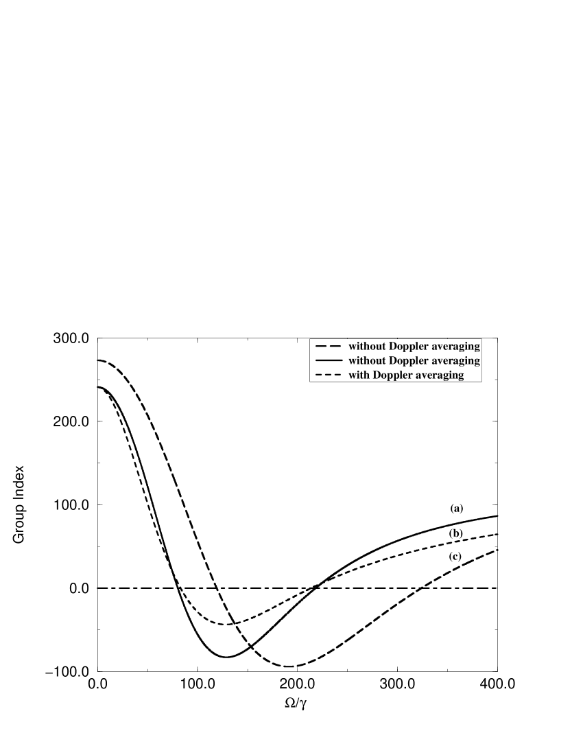
FIG. 2.: Group index variation with the Rabi frequency of LL coupling field. The curves (a) and (b) are for propagation in Rubidium vapor with density N$=2*10^{12}$ atoms/cc. Other parameters are chosen as G$=200\gamma$, $\Delta_{1}=\Delta_{2}=\Delta_{3}=0$, $\Gamma_{12}=\Gamma_{13}=\Gamma_{23}=0$, $\gamma=3*\pi*10^{6}$ rad/sec. For the curve (b) the Doppler width parameter $\delta$ is chosen as $1.33*10^{9}$ rad/sec. Curve (c) shows variation of group index $n_{g}$ with the Rabi frequency of LL coupling field in ²⁰⁸Pb vapor with density N$=2*10^{14}$ atoms/cc, G$=297\gamma$, $\Delta_{1}=\Delta_{2}=\Delta_{3}=0$, $\Gamma_{12}=\Gamma_{13}=\Gamma_{23}=0$, $\gamma=4.75*10^{7}$ rad/sec.

REFERENCES

- [1] A. Kasapi, M. Jain, G. Y. Yin, and S. E. Harris, Phys. Rev. Lett. 74, 2447 (1995).
- [2] O. Schmidt, R. Wynands, Z. Hussein, and D. Meschede, Phys. Rev. A 53, R27 (1996).
- [3] L. V. Hau, S. E. Harris, Z. Dutton, and C. H. Behroozi, Nature (London) 397, 594 (1999).
- [4] M. M. Kash, V. A. Sautenkov, A. S. Zibrov, L. Hollberg, G. R. Welch, M. D .Lukin, Y. Rostovtsev, E. S. Fry, and M. O. Scully, Phys. Rev. Lett. 82, 5229 (1999).
- [5] D. Budker, D. F. Kimball, S. M. Rochester, and V. V. Yashchuk, Phys. Rev. Lett. 83, 1767 (1999).
- [6] L. J. Wang, A. Kuzmich, and A. Dogariu, Nature (London) 406, 277 (2000); A. Dogariu, A.Kuzmich, and L. J. Wang, Phys. Rev. A 63, 053806 (2001).
- [7] For an early measurement see S. Chu and S. Wong, Phys. Rev. Lett. 48, 738 (1982); a very recent publication [Talukder et. al., Phys. Rev. Lett. 86, 3546 (2001)] also discusses the transition from subluminal to superluminal in propagation through a resonantly absorbing medium.
- [8] Ref. 5 also reports negative group delays near the center of the transition group.
- [9] S. E. Harris, J. E. Field, and A. Kasapi, Phys. Rev. A 46, R29 (1992).
- [10] S. E. Harris, Phys. Today 50, 36 (1997); S. E. Harris, J. E. Field, and A. Imamoğlu, Phys. Rev. Lett. 64, 1107 (1990).
- [11] L. Brillouin, Wave Propagation and Group Velocity (Academic, New York, 1960).
- [12] M. Xiao, Y. Q. Li, S. Z. Jin, and J. Gea-Banacloche, Phys. Rev. Lett. 74, 666 (1995).
- [13] R. Y. Chiao, Phys. Rev. A 48, R34 (1993); E. L. Bloda, R. Y. Chiao, and J. C. Garrison, Phys. Rev. A 48, 3890 (1993).
- [14] E. Bloda, J. C. Garrison, and R. Y. Chiao, Phys. Rev. A 49, 2938 (1994).
- [15] M. W. Mitchell and R. Y. Chiao, Am. J. Phys. 66, 14 (1998).
- [16] A. M. Steinberg and R. Y. Chiao, Phys. Rev. A 49, 2071 (1994).
- [17] A. M. Akulshin, S. Barreiro, and A. Lezama, Phys. Rev. Lett. 83, 4277 (1999); D. L. Fisher and T. Tajima, Phys. Rev. Lett. 71, 4338 (1993).
- [18] J. L. Bowie, J. C. Garrison, and R. Y. Chiao, Phys. Rev. A 61, 053811 (2000).
- [19] Sunish Menon and G. S. Agarwal, Phys. Rev. A 59, 740 (1999). The cross talk produces regions in linear response where one would have superluminal propagation [Sunish Menon, Ph. D. Thesis, submitted to Mohanlal Sukhadia University, Udaipur, India (to be published)].
- [20] We note that emission of coherent microwave radiation under coherent population trapping has been observed [A. Godone, F. Levi, and J. Vanier, Phys. Rev. A 59, R12 (1999)].
- [21] D. Bortman-Arbiv, A. D. Wilson-Gordon, and H. Friedmann, [Phys. Rev. A 63, 043818 (2001)] report superluminal propagation with in an absorption line by considering propagation in a -system with two upper states connected by a microwave field.
- [22] Budker et. al. noted in Ref. 5 how the propagation can be changed from subluminal to superluminal by using, say, static magnetic fields of the order of few .
- [23] C. G. B. Garrett and D. E. McCumber, Phys. Rev. A 1, 305 (1970).
- [24] In the experiment of Wang et. al. similar regions of were used to produce superluminal propagation.