Probabilistic implementation of universal quantum processors

Abstract

We present a probabilistic quantum processor for qudits. The processor itself is represented by a fixed array of gates. The input of the processor consists of two registers. In the program register the set of instructions (program) is encoded. This program is applied to the data register. The processor can perform any operation on a single qudit of the dimension $N$ with a certain probability. If the operation is unitary, the probability is in general $1/N^{2}$, but for more restricted sets of operators the probability can be higher. In fact, this probability can be independent of the dimension of the qudit Hilbert space of the qudit under some conditions.

I Introduction

Schematically we can represent a classical computer as a device with a processor, which is a fixed piece of hardware, that performs operations on a data register according to a program encoded initially in the program register. The action of the processor is fully determined by the program. The processor is universal if we can realize any operation on the data by entering the appropriate program into the program register.

In this paper we shall examine a quantum version of this picture. Specifically, in close analogy with recent papers by Nielsen and Chuang [1] and Vidal and Cirac [2], we will study how a quantum program initially put into a program register can cause a particular operation to be applied to a data register initially prepared in an unknown state. We shall first consider the case in which the data consists of a single qubit, and the program of two qubits. We shall then examine higher-dimensional systems.

Nielsen and Chuang [1] originally formulated the problem in terms of a programmable array of quantum gates, which can be described as a fixed unitary operator, ${P}_{dp}$, that acts on both the program and the data. The initial state, $|\Xi_{U}\rangle_{p}$, of the program register stores information about the one-qubit unitary transformation ${U}$ that is going to be performed on a single-qubit data register initially prepared in a state $|\psi\rangle_{d}$. The total dynamics of the programmable quantum gate array is then given by

$${P}_{dp}\left[|\psi\rangle_{d}\otimes|\Xi_{U}\rangle_{p}\right]=\left(U|\psi\rangle_{d}\right)\otimes|\tilde{\Xi}_{U}\rangle_{p},$$ (1)

where only pure data states were considered. The program register at the output of the gate is in the state $|\tilde{\Xi}_{U}\rangle_{p}$ - which was shown to be independent of the input data state $|\psi\rangle_{d}$.

Nielsen and Chuang proved that any two inequivalent operations $U$ and $V$ require orthogonal program states, i.e. $\langle\Xi_{U}|\Xi_{V}\rangle=0$. Thus, in order to perfectly implement a set of inequivalent operations,$\{U_{j}|j\in J\}$, the state space for the program register must contain the orthonormal set of program states, $\{|\Xi_{U_{j}}\rangle|j\in J\}$. This means that the dimension of the program register must be at least as great as the number of unitary operators that we want to perform. Since the set of unitary operations is infinite, the result of Nielsen and Chuang implies that no universal gate array can be constructed using finite resources, that is, with a finite dimensional program register. They did show, however, that if the gate array is probabilistic, a universal gate array is possible. A probabilistic array is one that requires a measurement to be made at the output of the program register, and the output of the data register is only accepted if a particular result, or set of results, is obtained. This will happen with a probability, which is less than one.

Vidal and Cirac [2] have recently presented a probabilistic programmable quantum gate array with a finite program register, which can realize a one parameter family of operations, where the parameter is continuous, with arbitrarily high probability. The higher the probability of success, the greater the dimensionality of the program register, but the number of transformations that can be realized is infinite. They have also considered approximate programmable quantum gate arrays, which perform an operation $E_{U}$ very similar to the desired $U$, that is $F(E_{U},U)\geq 1-\epsilon$ for some transformation fidelity $F$.

Another aspect of the encoding of quantum operations in the states of program registers has been discussed by Huelga and coworkers [3]. In this paper the implementation of an arbitrary unitary operation $U$ upon a distant quantum system has been considered. This so called teleportation of unitary operations has been formally represented as a completely positive, linear, trace preserving map on the set of density operators of the program and data registers:

$${\cal T}\left[|\xi\rangle_{ab}\otimes|\Xi_{U}\rangle_{p}\otimes|\psi\rangle_{d}\right]=|\tilde{\xi}_{U}\rangle_{ap}\otimes\left(U|\psi\rangle_{d}\right)$$ (2)

Here $|\xi\rangle_{a}$ represents a specific entangled state that is shared by two parties, Alice and Bob, who want to teleport the unitary operation $U$ from Alice to Bob. Huelga et al. [3] have investigated protocols which achieve the teleportation of $U$ using local operations, classical communication and shared entanglement.

In the present paper we will address the problem of implementing an operation $U$, encoded in the state of a program register $|\Xi_{U}\rangle_{p}$, on the data state $|\psi\rangle_{d}$. The gate arrays we present are probabilistic; the program register must be measured at the end of the procedure. In Section II we present a simple example of how to apply an arbitrary operation to a single qubit initially prepared in a state $|\psi\rangle$. The gate array consists of four Controlled-NOT (C-NOT) gates, and can implement four programs perfectly. These programs cause the one of the operations $\openone$, $\sigma_{x}$, $-i\sigma_{y}$, or $\sigma_{z}$ to be performed on the data qubit. Here $\openone$ is the identity and $\sigma_{j}$, where $j=x,y,z$ is a Pauli matrix. By choosing programs that are linear combinations of the four basic ones, it is possible to probabilistically perform any linear operation on the data qubit. In Section III we generalize the idea to an arbitrary dimensional quantum system, a qudit.

II Operations on qubits

We would like to construct a device that will do the following: The input consists of a qubit, $|\psi\rangle_{d}$, and a second state, $|\Xi_{U}\rangle_{p}$, which may be a multiqubit state, that acts as a program. The output of the device will be a state $U|\psi\rangle_{d}$, where $U$ is an operation that is specified by $|\Xi_{U}\rangle_{p}$. In order to make this a little less abstract, we first consider an example: Let $|\phi\rangle$ and $|\phi_{\perp}\rangle$ be two orthogonal qubit states, and suppose that we want to perform the operation

$$A_{z}=|\phi_{\perp}\rangle\langle\phi_{\perp}|-|\phi\rangle\langle\phi|=\openone-2|\phi\rangle\langle\phi|,$$ (3)

on $|\psi\rangle_{d}$. The action of this operator is analogous to that of $\sigma_{z}$ in the basis $\{|0\rangle,|1\rangle\}$, except that it acts in the basis $\{|\phi_{\perp}\rangle,|\phi\rangle\}$. That is, $\sigma_{z}$ does nothing to $|0\rangle$ and multiplies $|1\rangle$ by $-1$, while $A_{z}$ does nothing to $|\phi_{\perp}\rangle$ and multiplies $|\phi\rangle$ by $-1$. Can we find a network and a program vector to implement this operation on $|\psi\rangle_{d}$?

We can, in fact, do this by using the network for a quantum information distributor (QID) as introduced in Ref. [4] (this is a modification of the quantum cloning transformation [5, 6] ). In this network the program register is represented by a two qubit state $|\Xi_{A}\rangle_{p}$. Before we present the network for the programmable gate array, we shall introduce notation for its components. A Controlled-NOT gate $D_{jk}$ acting on qubits $j$ and $k$ performs the transformation,

$$D_{jk}|m\rangle_{j}|n\rangle_{k}=|m\rangle_{j}|m\oplus n\rangle_{k},$$ (4)

where $j$ is the control bit, $k$ is the target bit, and $m$ and $n$ are either $0$ or $1$. The addition is modulo $2$. The QID network consists of four Controlled-NOT gates, and acts on three qubits (a single data qubit denoted by a subscript 1 and two program qubits denoted by subscripts 2 and 3, respectively). Its action is given by the operator $P_{123}=D_{31}D_{21}D_{13}D_{12}$. As our first task, we shall determine how this network acts on input states where qubit $1$ is in the state $|\psi\rangle$, and qubits $2$ and $3$ are in Bell basis states. The Bell basis states are defined by

$$|\Phi_{+}\rangle = \frac{1}{\sqrt{2}}(|01\rangle+|10\rangle)\equiv|\Xi_{01}\rangle\,,$$ (5)

$$|\Phi_{-}\rangle = \frac{1}{\sqrt{2}}(|01\rangle-|10\rangle)\equiv|\Xi_{11}\rangle\,;$$ (6)

$$|\Psi_{+}\rangle = \frac{1}{\sqrt{2}}(|00\rangle+|11\rangle)\equiv|\Xi_{00}\rangle\,;$$ (7)

$$|\Psi_{-}\rangle = \frac{1}{\sqrt{2}}(|00\rangle-|11\rangle)\equiv|\Xi_{10}\rangle\,.$$ (8)

We find that

$$P_{123}|\psi\rangle_{1}|\Phi_{+}\rangle_{23} = (\sigma_{x}|\psi\rangle_{1})|\Phi_{+}\rangle\,;$$ (9)

$$P_{123}|\psi\rangle_{1}|\Phi_{-}\rangle_{23} = (-i\sigma_{y}|\psi\rangle_{1})|\Phi_{-}\rangle\,;$$ (10)

$$P_{123}|\psi\rangle_{1}|\Psi_{+}\rangle_{23} = |\psi\rangle_{1}|\Psi_{+}\rangle\,;$$ (11)

$$P_{123}|\psi\rangle_{1}|\Psi_{-}\rangle_{23} = (\sigma_{z}|\psi\rangle_{1})|\Psi_{-}\rangle.$$ (12)

Any operation on qubits can be expanded in terms of Pauli matrixes and the identity. The above equations mean that the Bell basis vectors are “programs” for a complete set of operations. In order to see how to make use of this, let us expand our proposed operation in terms of this complete set. Expressing $|\phi\rangle$ as $|\phi\rangle=\mu|0\rangle+\nu|1\rangle$, we have that

$$A_{z} = \openone-2|\phi\rangle\langle\phi|=\left(\begin{array}[]{cc}|\nu|^{2}-|\mu|^{2}&-2\mu\nu^{\ast}\\ -2\mu^{\ast}\nu&|\mu|^{2}-|\nu|^{2}\end{array}\right),$$ (15)

$$= -(\mu\nu^{\ast}+\mu^{\ast}\nu)\sigma_{x}+(\mu\nu^{\ast}-\mu^{\ast}\nu)(-i\sigma_{y})$$ (17)

$$+(|\nu|^{2}-|\mu|^{2})\sigma_{z}.$$

We can now apply the operation $A$ to $|\psi\rangle$ by sending in the “program” vector

$$|\Xi_{A}\rangle_{23}= - (\mu\nu^{\ast}+\mu^{\ast}\nu)|\Phi_{+}\rangle_{23}+(\mu\nu^{\ast}-\mu^{\ast}\nu)|\Phi_{-}\rangle_{23}$$ (18)

$$+ (|\nu|^{2}-|\mu|^{2})|\Psi_{-}\rangle_{23},$$ (19)

and measuring the program outputs in order to determine if they are in the state $(|\Phi_{+}\rangle+|\Phi_{-}\rangle+|\Psi_{-}\rangle)/\sqrt{3}$. If they are, our operation has been accomplished. Note that the measurement is independent of the vector $|\phi\rangle$ so that no knowledge of this vector is necessary to make the measurement and to determine whether the procedure has been successful. As we see, the probability of success is 1/3 for the implementation of the operation $A_{z}$ which is parameterized in general by two continuous parameters (i.e. the state $|\phi\rangle$).

Let us examine the program vector more carefully. If we define the unitary operation, $U_{init}$, by

$$U_{init}|00\rangle = -|10\rangle\,;\qquad U_{init}|10\rangle=-|11\rangle\,;$$ (20)

$$U_{init}|11\rangle = |01\rangle\,;\qquad U_{init}|01\rangle=|00\rangle\,;$$ (21)

we have that

$$|\Xi_{A}\rangle_{12}=U_{init}\frac{1}{\sqrt{2}}(|\phi\rangle|\phi_{\perp}\rangle+|\phi_{\perp}\rangle|\phi\rangle).$$ (22)

Finally, we can summarize our procedure. The steps are

  1.

Start with the state $\frac{1}{\sqrt{2}}(|\phi\rangle|\phi_{\perp}\rangle+|\phi_{\perp}\rangle|\phi\rangle)$ .

  2.

Apply $U_{init}$.

  3.

Send the resulting state into the control ports (inputs $2$ and $3$) and $|\psi\rangle$ into port 1.

  4.

Measure $(|\Phi_{+}\rangle+|\Phi_{-}\rangle+|\Psi_{-}\rangle)/\sqrt{3}$ at the output of the control ports.

  5.

If the result is yes, then the output of port $1$ is $(\openone-2|\phi\rangle\langle\phi|)|\psi\rangle$.

Before proceeding to a more general consideration of this network, let us make an observation. Suppose that we carry out the same procedure, but instead of starting with the program vector $(|\phi\rangle|\phi_{\perp}\rangle+|\phi_{\perp}\rangle|\phi\rangle)/\sqrt{2}$, we start instead with the program vector $(|\phi\rangle|\phi\rangle-|\phi_{\perp}\rangle|\phi_{\perp}\rangle)/\sqrt{2}$. At the end of the procedure the output of the data register is $A_{x}|\psi\rangle$, where

$$A_{x}=|\phi\rangle\langle\phi_{\perp}|+|\phi_{\perp}\rangle\langle\phi|.$$ (23)

The operation $A_{x}$ interchanges $|\phi\rangle$ and $|\phi_{\perp}\rangle$. Its action is analogous to that of $\sigma_{x}$, which interchanges the vectors $|0\rangle$ and $|1\rangle$. The probability of success for this procedure is also $1/3$.

We now need to determine whether there is a program for any operator that could act on $|\psi\rangle$. The operator need not be unitary; it could be a result of coupling $|\psi\rangle$ to an ancilla, evolving the coupled system (a unitary process), and then measuring the ancilla. Therefore, if $A$ is now any linear operator acting on a two dimensional quantum system, the transformations in which we are interested are given by

$$|\psi\rangle\rightarrow\frac{1}{\|A\psi\|}A|\psi\rangle.$$ (24)

Let us denote the operators, which can be implemented by Bell state programs, by $S_{00}=\openone$, $S_{01}=\sigma_{x}$, $S_{10}=\sigma_{z}$, and $S_{11}=-i\sigma_{y}$. Any $2\times 2$ matrix can be expanded in terms of these operators, so that we have

$$A=\sum_{j,k=0}^{1}\tilde{a}_{jk}S_{jk}.$$ (25)

We now define $a_{jk}=\tilde{a}_{jk}/\sqrt{\eta}$, where

$$\eta=\sum_{j,k=0}^{1}|\tilde{a}_{jk}|^{2},$$ (26)

so that

$$1=\sum_{j,k=0}^{1}|a_{jk}|^{2}.$$ (27)

Now let us go back to our network and consider the program vector given by

$$|\Xi_{A}\rangle=\sum_{j,k=0}^{1}a_{jk}|\Xi_{jk}\rangle,$$ (28)

and at the output of the program register we shall measure the projection operator corresponding to the vector $(1/2)\sum_{j,k=0}^{1}|\Xi_{jk}\rangle$. If the measurement is successful, the state of the data register is, up to normalization, given by

$$|\psi\rangle\rightarrow\left(\sum_{j,k=0}^{1}a_{jk}S_{jk}\right)|\psi\rangle\,.$$ (29)

After this state is normalized, it is just $(1/\|A\psi\|)|\psi\rangle$. This means that for any transformation of the type given in Eq. (24), we can find a program for our network that will carry it out.

III Generalization to qudits

In order to extend the network presented in the previous section to higher dimensions, we must first introduce a generalization of the two-qubit C-NOT gate [4] (see also Ref. [7]). As we noted previously, it is possible express the action of a C-NOT gate as a two-qubit operator of the form

$${D}_{ab}=\sum_{k,m=0}^{1}|k\rangle_{a}\langle k|\otimes|m\oplus k\rangle_{b}\langle m|\;.$$ (30)

In principle one can also introduce an operator ${D}^{\dagger}_{ab}$ defined as

$${D}^{\dagger}_{ab}=\sum_{k,m=0}^{1}|k\rangle_{a}\langle k|\otimes|m\ominus k\rangle_{b}\langle m|\;.$$ (31)

In the case of qubits these two operators are equal, but this will not be the case when we generalize the operator to Hilbert spaces whose dimension is larger than 2 [4, 7]. In particular, we can generalize the operator ${D}$ for dimension $N>2$ by defining

$${D}_{ab}=\sum_{k,m=0}^{N-1}|k\rangle_{a}\langle k|\otimes|(m+k){\rm mod}\,N\rangle_{b}\langle m|\;,$$ (32)

which implies that

$${D}_{ab}^{\dagger}=\sum_{k,m=0}^{N-1}|k\rangle_{a}\langle k|\otimes|(m-k){\rm mod}\,N\rangle_{b}\langle m|\;.$$ (33)

From this definition it follows that the operator ${D}_{ab}$ acts on the basis vectors as

$${D}_{ab}|k\rangle|m\rangle=|k\rangle|(k+m){\rm mod}\,N\rangle\;,$$ (34)

which means that this operator has the same action as the conditional adder and can be performed with the help of the simple quantum network discussed in [8]. Now we see that for $N>2$ the two operators $D$ and ${D}^{\dagger}$ do differ; they describe conditional shifts in opposite directions. Therefore the generalizations of the C-NOT operator to higher dimensions are just conditional shifts.

In analogy with the quantum computational network discussed in the previous section, we assume the network for the probabilistic universal quantum processor to be

$${P}_{123}={D}_{31}{D}_{21}^{\dagger}{D}_{13}{D}_{12}\;.$$ (35)

The data register consists of system $1$ and the program register of systems $2$ and $3$. The state $|\Xi_{U}\rangle_{23}$ acts as the “software” which the operation to be implemented on the qudit data state $|\Psi\rangle_{1}$. The output state of the three qudit system, after the four controlled shifts are applied, reads

$$|\Omega\rangle_{123}={D}_{31}{D}_{21}^{\dagger}{D}_{13}{D}_{12}|\Psi\rangle_{1}|\Xi_{U}\rangle_{23}\;.$$ (36)

A graphical representation of the logical network (36) with the conditional shift gates ${D}_{ab}$ in Fig. 1.

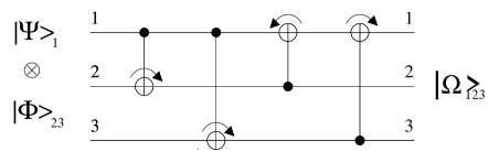
FIG. 1.: A logic network for the universal quantum processor as given by the unitary transformation (36). The action of the controlled shift operator $D_{jk}$ is represented as follows: The control qudit is represented by $\bullet$ while the target qudit is represented $\oplus$ with the rightarrow. The action of the operator $D_{jk}^{\dagger}$ is represented by left arrow.

The sequence of four operators acting on the basis vectors gives $|n\rangle_{1}|m\rangle_{2}|k\rangle_{3}$ as

  

$${D}_{31}{D}_{21}^{\dagger}{D}_{13}{D}_{12}|n\rangle_{1}|m\rangle_{2}|k\rangle_{3}=|(n-m+k){\rm mod}\,N\rangle_{1}\,|(m+n){\rm mod}\,N\rangle_{2}\,|(k+n){\rm mod}\,N\rangle_{3}\;.$$ (37)

  

We now turn to the fundamental program states. A basis consisting of maximally entangled two-particle states (the analogue of the Bell basis for spin-$\frac{1}{2}$ particles) is given by [9]

$$|\Xi_{mn}\rangle=\frac{1}{\sqrt{N}}\sum_{k=0}^{N-1}\exp\Bigl{(}i\frac{2\pi}{N}mk\Bigr{)}|k\rangle|(k-n){\rm mod}\,N\rangle\,,\!\!\!$$ (38)

where $m,n=0,\dots,N-1$. If $|\Xi_{mn}\rangle_{p}$ is the initial state of the program register, and $|\Psi\rangle=\sum_{j}\alpha_{j}|j\rangle_{d}$ (here, as usual, $\sum_{j}|\alpha_{j}|^{2}=1$) is the initial state of the data register, it then follows that

$${P}_{123}|\Psi\rangle_{1}|\Xi_{mn}\rangle_{23}=$$ (39)

$$= \sum_{jk}\frac{\alpha_{j}}{\sqrt{N}}\exp\frac{2\pi ikm}{N}{P}_{123}|j\rangle|k\rangle|k-n\rangle$$ (40)

$$= \sum_{jk}\frac{\alpha_{j}}{\sqrt{N}}\exp\frac{2\pi ikm}{N}|j-n\rangle|k+j\rangle|k+j-n\rangle$$ (41)

$$= \sum_{jk}\alpha_{j}\exp\frac{-2\pi ijm}{N}|j-n\rangle|\Xi_{mn}\rangle$$ (42)

$$= (U^{(mn)}|\Psi\rangle)|\Xi_{mn}\rangle,$$ (43)

where we have introduced the notation

$$U^{(mn)}=\sum_{s=0}^{N-1}\exp\frac{-2i\pi sm}{N}|s-n\rangle\langle s|.$$ (44)

This result is similar to the one we found in the case of a single qubit. We would now like to examine which transformations we can perform on the state in the data register by using a program consisting of a linear combination of the vectors $|\Xi_{mn}\rangle$ followed by the action of the processor ${P}_{123}$ and a subsequent measurement of the program register.

The operators $U^{(mn)}$ satisfy the orthogonality relation

$${\rm Tr}\left[(U^{(m^{\prime}n^{\prime})})^{\dagger}U^{(mn)}\right]=N\delta_{mm^{\prime}}\delta_{nn^{\prime}}.$$ (45)

The space of linear operators ${\cal T}({\cal H})$ defined on some Hilbert space $\cal H$ with the scalar product given by (45) we know as Hilbert-Schmidt space. Thus the unitary operators $U^{(mn)}$ form an orthogonal basis in it and any operator $A\in{\cal T}({\cal H})$ can be expressed in terms of them

$$A=\sum_{m,n=0}^{N-1}q_{mn}U^{(mn)}.$$ (46)

The orthogonality relation allows us to find the expansion coefficients in terms of the operators

$$q_{mn}=\frac{1}{N}{\rm Tr}\left[\left(U^{(mn)}\right)^{\dagger}A\right].$$ (47)

Equations (45) and (46) imply that

$$\sum_{m,n=0}^{N-1}|q_{mn}|^{2}=\frac{1}{N}{\rm Tr}(A^{\dagger}A).$$ (48)

Therefore, the program vector that implements the operator $A$ is given by

$$|v_{A}\rangle_{23}=\left[\frac{N}{{\rm Tr}(A^{\dagger}A)}\right]^{1/2}\sum_{m,n=0}^{N-1}q_{mn}|\Xi_{mn}\rangle_{23}.$$ (49)

Application of the processor to the input state $|\Psi\rangle_{1}|v_{A}\rangle_{23}$ yields the output state

$$|\Omega\rangle_{123}=\sum_{mn}q_{mn}U^{(mn)}|\Psi\rangle_{1}\otimes|\Xi_{mn}\rangle_{23}.$$ (50)

To obtain the final result we perform a projective measurement of the program register onto vector $|M\rangle_{23}$

$$|M\rangle=\frac{1}{N}\sum_{m,n=0}^{N-1}|\Xi_{mn}\rangle$$ (51)

If the outcome of the measurement is positive, then we get the required transformation $A$ acting on an unknown, arbitrary input state $|\Psi\rangle_{1}$.

Let us consider an example. Suppose we choose for $A$ the unitary operator $\openone-2|\phi\rangle\langle\phi|$, where the normalized state $|\phi\rangle$ can be expressed as

$$|\phi\rangle=\sum_{k=0}^{N-1}\beta_{k}|k\rangle.$$ (52)

The expansion coefficients for this operation are given by

$$q_{mn}=\delta_{m0}\delta_{n0}-\frac{2}{N}\sum_{k=0}^{N-1}e^{2\pi ikm/N}\beta_{k}^{\ast}\beta_{k-n},$$ (53)

and the program vector for this operation is

$$|\Phi\rangle_{23}=|\Xi_{00}\rangle_{23}-\frac{2}{\sqrt{N}}\sum_{k,n=0}^{N-1}\beta^{\ast}_{-k}\beta_{-(k+n)}|k\rangle_{2}|k-n\rangle_{3}.$$ (54)

The program vector can be obtained from a state more closely related to $|\phi\rangle$ if we introduce a new unitary operator and a “complex conjugate” vector. Define the operator $W$ by

$$W|k\rangle=|-k\rangle,$$ (55)

and the vector $|\phi^{\ast}\rangle$ by

$$|\phi^{\ast}\rangle=\sum_{k=0}^{N-1}\beta^{\ast}_{k}|k\rangle.$$ (56)

We then have that

$$|\Phi\rangle_{23}=(W_{2}\otimes\openone_{3})\left(D_{23}^{\dagger}\right)^{2}\left(|\Xi_{00}\rangle_{23}-\frac{2}{\sqrt{N}}|\phi^{\ast}\rangle_{2}|\phi\rangle_{3}\right).$$ (57)

A network that performs the operation $(W_{2}\otimes\openone_{3})\left(D_{23}^{\dagger}\right)^{2}$ could be added to the input of the program register so that the simpler state that appears on the right-hand side of Eq. (57) could be used as the program. At the output of the processor we have to perform the projective measurement discussed in the previous paragraph, and the probability of achieving the desired result is the same as the probability of successfully implementing the transformation, $A$. In this case the probability is $1/N^{2}$.

IV Success Probability

The probability, $p$, of successfully applying the operator $A$ to the state $|\Psi\rangle_{1}$ in our example is rather small. This is because the operator we chose was a linear combination of all of the operators $U^{(mn)}$. This means that if the data register consists of $l$ qubits, i.e. $N=2^{l}$, then the probability of a successful implementation of a general transformation $A$ decreases exponentially with the size of the data register. However, if we were to choose an operator, or set of operators, that was a linear combination of only a few of the $U^{(mn)}$, then the success probability can be significantly improved. This would entail making a different measurement at the output of the program register. Instead of making a projective measurement onto the vector $|M\rangle$, one would instead make a measurement onto the vector

$$|M^{\prime}\rangle=\frac{1}{{\cal N}^{1/2}}\sum_{m,n:q_{mn}\neq 0}|\Xi_{mn}\rangle$$ (58)

where ${\cal N}$ is the total number of nonzero coefficients $q_{mn}$, in the decomposition in Eq. (46). If the operation being implemented is unitary, then, in this case, the probability of implementing it is

$$p=\frac{1}{\cal N}.$$ (59)

where ${\cal N}$ is the total number of nonzero coefficients $q_{mn}$, in the decomposition (46). There are, in fact, large classes of operations that can be expressed in terms of a small number of operators $U^{(mn)}$ [10]. For these operators, the probability of success can be relatively large and, in principle, independent of the size of the Hilbert space of the data register.

Example 1.
Let us consider the one-parameter set of unitary transformations $U_{\varphi}$

$$U_{\varphi}=\cos\varphi\,\openone+i\sin\varphi\,\left[\frac{1+i}{2}U^{(01)}+\frac{1-i}{2}U^{(03)}\right]$$ (60)

where the unitaries $U^{(mn)}$ are given by Eq.(44). These unitaries for $N=4$ can be explicitly written as

$$U^{(01)}=\sum_{s=0}^{3}(-i)^{s}P_{s}\,;\qquad U^{(03)}=\sum_{s=0}^{3}(i)^{s}P_{s}\,,$$ (61)

where $P_{s}=|s\rangle\langle s|$. From here we find the expression for the operator (60) in the form:

$$U_{\varphi}=\cos\varphi\,\openone+i\sin\varphi\,\left[P_{0}+P_{1}-P_{2}-P_{3}\right]\,,$$ (62)

We note that if we rewrite the parameters $s$ as binary numbers, $s=j_{1}2+j_{0}$, where $j_{k}$ is either $0$ or $1$, and express the states $|s\rangle$ as tensor products of qubits, i.e. $|s\rangle=|j_{1}\rangle\otimes|j_{0}\rangle$, we find that the operator in brackets on the right-hand side of Eq. (60) can be expressed as

$$\left[\frac{1+i}{2}U^{(01)}+\frac{1-i}{2}U^{(03)}\right]=\sigma_{3}\otimes\openone.$$ (63)

From Eq. (62) it is clear that $U_{\varphi}$ has eigenvalues of magnitude $1$, which implies that $U_{\varphi}$ is unitary. It can be realized by the universal quantum processor (35) with a probability of successful implementation equal to $1/3$. This example illustrates that it is possible to realize large classes of unitary operations with a probability that is greater than the reciprocal of the dimension of the program register.

This example can be easily generalized. Consider a one-parameter set of unitary operators acting on a Hilbert space consisting of $l$ qubits, which is given by

$$U_{\varphi}=\cos\varphi\,\openone^{\otimes l}+i\sin\varphi\,\sigma_{3}\otimes\openone^{\otimes(l-1)}$$ (64)

The operator $\sigma_{3}\otimes\openone^{\otimes(l-1)}$ is diagonal and therefore only the diagonal unitaries from our set $U^{(mn)}$, i.e. $U^{(m0)}$, appear in its expansion, Eq. (46) . Moreover the coefficients $q_{m0}$ in the expansion are non-vanishing only for odd $m$. It follows that

$$U_{\varphi}=\cos\varphi\,\openone^{\otimes l}+i\sin\varphi\,\sum_{{\rm odd}\ m}q_{m0}U^{(m0)},$$ (65)

and the probability of a successful implementation of this unitary transformation is $p=2/(2^{l}+2)$.

Example 2.
For some sets of operators it is possible to do even better than we were able to do in the previous example. Consider the one-parameter set of unitary operators given by

$$U_{\vartheta}=\cos\vartheta\,\openone+i\sin\vartheta\,U^{(0,N/2)},$$ (66)

where $N$ is assumed to be even. That this operator is unitary follows from the fact that $U^{(0,N/2)}$ is self-adjoint. A program vector that would implement this operator is

$$|\Phi\rangle_{23}=\cos\vartheta|\Xi_{00}\rangle_{23}+i\sin\vartheta|\Xi_{0,N/2}\rangle_{23},$$ (67)

and at the output of the program register we make a projective measurement corresponding to the vector

$$|M\rangle_{23}=\frac{1}{\sqrt{2}}(|\Xi_{00}\rangle_{23}+|\Xi_{0,N/2}\rangle_{23}.$$ (68)

The probability for successfully achieving the desired result, i.e. the vector $U_{\vartheta}|\Psi\rangle_{1}$ in the data register, is $1/2$ irrespective of the value $N$, i.e. the number of qubits.

V Conclusion

We have presented here a programmable quantum processor that exactly implements a set of operators that form a basis for the space of operators on qudits. This processor has a particularly simple representation in terms of elementary quantum gates. It is, however, by no means unique. It is possible, in principle, to build a processor that exactly implements any set of unitary operators that form a basis for the set of operators on qudits of dimension $N$, and uses any orthonormal set of $N^{2}$ vectors as programs. Explicitly, if the set of operators is $\{V_{n}|n=1,\ldots N^{2}\}$ and the program vectors are $\{|y_{n}\rangle|n=1,\ldots N^{2}\}$, the processor transformation is given by

$$P_{dp}=\sum_{n=1}^{N^{2}}V_{n}^{(d)}\otimes|y_{n}\rangle_{p}\,{}_{p}\langle y_{n}|,$$ (69)

where the superscript $(d)$ on the operator $V_{n}$ indicates that it acts on the data register.

As an example, consider a data register consisting of $l$ qubits. We could use the processor discussed in section III to perform operations on states in this register, but we can also do something else; we can use $l$ single-qubit processors, one for each qubit of the data register. Specifically, our unitary basis for the set operations on the data register would be

$$U_{JK}=U_{j_{1}k_{1},\dots,j_{l}k_{l}}=\bigotimes_{m=1}^{l}S_{j_{m}k_{m}}$$ (70)

where $J=(j_{1},\dots,j_{l})$ and $K=(k_{1}\dots,k_{l})$ are sequences of zeros and ones, and the operators $S_{j_{m}k_{m}}$ are the defined immediately after Eq. (24). The program register would consist of $l$ pairs of qubits, $2l$ qubits in all, with each pair controlling the operation on one of the qubits in the data register. Each of the operators in our basis can be implemented perfectly by a program consisting of the tensor product state, $\prod_{m=0}^{l}|\Xi_{j_{m}k_{m}}^{(m)}\rangle$, where $|\Xi_{j_{m}k_{m}}^{(m)}\rangle$ is a two-qubit state that implements the operation $S_{j_{m}k_{m}}$ on the $m$th qubit of the data register.

We are then faced with the problem of which processor to use. This very much depends on the set of operations we want to apply to the data. How to choose the processor so that a given set of operations can be implemented with the greatest probability, for a fixed size of the program register is an open problem. A second issue is simplicity. One would like the processor itself and the program states it uses to be as simple as possible. The simplicity of the processor is related to the number of quantum gates it takes to construct it. We would maintain that the processors we have presented here are simple, though whether there are simpler ones we do not know. Judging the simplicity of the program states is somewhat more difficult, but they should be related in a relatively straightforward way to the operation that they encode. In many cases these states will have been produced by a previous part of a quantum algorithm, and complicated program states will mean more complexity for the algorithm that produces them. The program states proposed by Vidal and Cirac and the ones proposed by us in section II are, in our opinion, simple.

A final open problem that we shall mention, is finding a systematic way of increasing the probability of successfully carrying out a set of operations by increasing the dimensionality of the space of program vectors. Vidal and Cirac showed how to do this in a particular case, but more general constructions would be desirable [2]. Doing so would give one a method of designing programs for a quantum computer.

- [1] M. A. Nielsen and I. L. Chuang, Phys. Rev. Lett. 79, 321 (1997)
- [2] G. Vidal and J.I. Cirac, Los Alamos arXiv quant-ph/0012067 (2000); see also G. Vidal, L. Masanes, and J.I. Cirac, Los Alamos arXiv quant-ph/0102037 (2001).
- [3] S. F. Huelga, J. A. Vaccaro, and A. Chefles, Los Alamos arXive quant-ph/0005061 v.3 (2000).
- [4] S. Braunstein, V. Bužek, and M. Hillery, Phys. Rev. A 63, 052313 (2001).
- [5] V. Bužek and M. Hillery, Phys. Rev. A 54, 1844 (1996).
- [6] V. Bužek, S. Braunstein, M. Hillery, and D. Bruß, Phys. Rev. A 56, 3446 (1997).
- [7] G. Alber, A. Delgado, N. Gisin, and I. Jex, Los Alamos arXive quant-ph/0008022.
- [8] V. Vedral, A. Barenco, and A. Ekert, Phys. Rev. A 54, 147 (1996).
- [9] D. I. Fivel, Phys. Rev. Lett. 74, 835 (1995).
- [10] We note that an arbitary sum of unitary operators is not necessarily a unitary operator.