Removal of a single photon by adaptive absorption

Abstract

We present a method to remove, using only linear optics, exactly one photon from a field-mode. This is achieved by putting the system in contact with an absorbing environment which is under continuous monitoring. A feedback mechanism then decouples the system from the environment as soon as the first photon is absorbed. We propose a possible scheme to implement this process and provide the theoretical tools to describe it.

I Introduction

In the last decades experimental technology has reached the point in which quantum effects cannot only be observed but also controlled. Sensors have become very precise and individual quantum systems can be manipulated through coupling to semiclassical driving fields. Despite this, we are still far from having full control over quantum systems. In the field of quantum optics, the two main reasons for this are that the coupling to the driving fields is in practice quite limited, and the non-desired coupling to the environment produces damping and decoherence effects which hinder controllability. Classical control theory has been quite successful in manipulating classical systems with complex or partially unknown dynamics. Classical control consists of closely monitoring the system, processing the measured data and applying the appropriate feedback signal to modify the evolution of the system. In the field of quantum optics this idea has been used to stabilize the phase or intensity of lasers. However, this reduction of noise could be explained classically.

Non-linear effects are used to reduce noise in the quantum domain. Yamamoto et al[1] presented the first scheme which relied only on feedback to generate photocurrents with noise below the standard quantum limit. Based on Langevin equations, Shapiro et al. [2] gave the first quantum and semiclassical descriptions of feedback control. Wiseman and coworkers [3] derived a closed-loop master equation describing the instantaneous feedback of a homodyne current measured outside an optical cavity. This work, based on quantum trajectories, made clear the connection between control and quantum measurement theory and made possible a complete understanding of ‘quantum-limited’ feedback. Subsequently several applications and elaborations of this first quantum theory of continuous feedback appeared. In general the feedback does not have to be instantaneous and can be a functional of the entire history of measurement results, thus typically resulting in a non-Markovian evolution. Doherty and Jacobs [4] showed that in determining the form of this functional it is useful to formulate feedback control in two steps: estimation of the state of the system, and application of appropriate control inputs to affect the dynamics. In [5] Doherty et al. extended this idea further to investigate how methods in the well developed classical control theory can apply quantum feedback control. From the application point of view, feedback has been proposed as a means to improve atom localization in standing waves [6, 4], cooling of cavity mirrors [7], controlling coherence of two-level atoms [8], inverting quantum jumps [9], line narrowing in atomic fluorescence [10], slowing down of decoherence effects [11], and preserving macroscopic superpositions of light fields [12].

In most of these applications, feedback is used to keep an open system under control. The back-action of measurement in the ‘quantum-limited’ feedback is nearly considered as a drawback, and the feedback is enforced by the action of a driving field that shapes the potential. In our proposal the feedback itself is used to create an otherwise difficult operation. In fact, the evolution is tailored only by the continuous measurement procedure.

The idea in this work is to show that feedback control implemented by simple linear optical elements can be of great use in manipulating quantum states of light. This is, at present, particularly interesting in the context of quantum communication where photons are the only serious qubit carriers. Their very weak coupling strengths suppress decoherence effects, but at the same time render rather difficult the implementation of quantum gates. Any tools which perform non-trivial tasks without relying on photon-photon interactions are therefore very desirable. The use of linear optical elements has already proven to facilitate some tasks [13]. Here, we address the particular problem of removing precisely one photon from a field mode. Our proposal is based on a very simple form of feedback and for its implementation only linear optical elements are needed. The central idea is that of adaptive absorption and consists of coupling the mode to an environment and monitoring that environment for the absorption of a photon. Once a photon has been detected the coupling to the environment is switched off. If the coupling is maintained until a photon has been absorbed, then this procedure removes exactly one photon from the field.

The paper is organized as follows. Section II briefly reviews the main properties of linear absorption. The master equation describing the evolution of the field in the absorber is introduced. These results are used in Section III where we give the evolution of the field in adaptive absorption, and in Section IV where we give a possible implementation. In Section V, we study the evolution under adaptive absorption for some relevant input states. Section VI treats the question obtaining information about the input field from the time at which the absorption occurs. Finally, in Section VII we present some further elaborations and conclude the paper.

II Linear absorption

Absorption in a linear medium is characterized by a reduction of optical field amplitude by a factor $\eta^{\frac{1}{2}}$ which is independent of the field amplitude. A coherent state $\left|\alpha\right>$ after being partially absorbed during its propagation through, for example, an optical fiber is transformed to $\left|\eta^{\frac{1}{2}}\alpha\right>$. This is formally the same relation as between the input and one of the output arms of a beam splitter. The P-representation (see Eq. (23) below) allows us to extend the previous formal analogy to all input states. The beam-splitter also serves as a model for phase-sensitive damping [14, 15] by feeding the second input port with a squeezed state.

The action of beam splitters is widely studied (see for example [16]). Some properties which are relevant in our context are: a) The output modes are in general entangled and therefore the transmitted state is a mixed state. b) Coherent states are an exception to the previous statement. c) When the vacuum and $n$ photons are fed into the input ports, the photon number distribution in the output ports follows the same statistical law for distributing $n$ classical particles: i.e. from $n$ photons the absorber will let through $m$ photons at random with probability $\eta$ for each, while absorbing $(m-n)$ with probability $1-\eta$. The resulting probability distribution for the transmitted field is,

$$p_{BS}(m)=\left(\begin{array}[]{c}n\\ m\end{array}\right)\eta^{m}(1-\eta)^{(n-m)}.$$ (1)

d) Vacuum fluctuations from the input port are added to the the transmitted field. This illustrates the fact that dissipation is always accompanied by extra fluctuations.

The beam splitter analogy gives us a relation between the input and output photonic states. While the field is in contact with the absorbing medium, its evolution is non-unitary because of the losses, but may be described by the master equation

$$\frac{d\rho}{dt}=\Gamma(2a\rho(t)a^{\dagger}-a^{\dagger}a\rho(t)-\rho(t)a^{\dagger}a)\mbox{,}$$ (2)

where $a$ is the annihilation operator of the field-mode. This is the master equation of a harmonic oscillator coupled to a broad-bandwidth bath [17]. It is useful to separate the evolution superoperator into two terms defined by

$$\hat{J}\rho = a\rho a^{\dagger}$$ (3)

$$\hat{L}\rho = -\frac{1}{2}[a^{\dagger}a\rho+\rho a^{\dagger}a]$$ (4)

The master equation (2) can now be rewritten in the compact form,

$$\dot{\rho}=2\Gamma(\hat{J}+\hat{L})\rho\mbox{.}$$ (5)

A solution of this differential equation may be expressed in a number of ways including [18],

$$\rho(t) = \sum_{m=0}^{\infty}\int_{0}^{t}\mbox{d}t_{m}\int_{0}^{t_{m}}\mbox{d}t_{m-1}\cdots\int_{0}^{t_{2}}\mbox{d}t_{1}\mbox{e}^{2\Gamma\hat{L}(t-t_{m})}$$ (6)

$$\times 2\Gamma\hat{J}\mbox{e}^{2\Gamma\hat{L}(t_{m}-t_{m-1})}\cdots 2\Gamma\hat{J}\mbox{e}^{2\Gamma\hat{L}t_{1}}\rho(0)$$ (7)

This formal solution allows for an interpretation in terms of conditioned evolution in agreement with quantum measurement theory. The solution is formed from terms of the form,

$$\bar{\rho_{c}}(t) = \exp[2\Gamma\hat{L}(t-t_{N})]2\Gamma\hat{J}\exp[2\Gamma\hat{L}(t_{N}-t_{N-1})]\cdots$$ (9)

$$\cdots 2\Gamma\hat{J}\exp[2\Gamma\hat{L}t_{1}]\rho(0)\mbox{.}$$

Each occurrence of $\hat{J}$ corresponds to the loss of a photon. The exponential terms account for the non-unitary evolution of the system between photon absorptions. It follows that

$$\rho_{c}(t)=\frac{\bar{\rho_{c}}(t)}{\mbox{Tr}\left(\bar{\rho_{c}}(t)\right)}$$ (10)

can be interpreted as the evolved density matrix conditioned by the loss of $N$ photons to the environment at times $t_{1},t_{2},\ldots,t_{N}$. The norm of $\bar{\rho_{c}}(t)$ gives the probability of this particular sequence of detections to occur. The unconditional evolution described in Eq. (7) is then obtained by averaging over all possible histories, i.e. summing over the number of lost photons $m$, and integrating over their corresponding absorption times $t_{1}\ldots t_{m}$. The action of the superoperator $\hat{J}$ is sometimes referred to as a ‘quantum jump’, since it produces a finite change in the state in an infinitesimal time. In contrast, when no quantum jump occurs, the change is infinitesimal but not unitary.

A coherent state after the loss of a photon and after a time $\Delta t$ without losses is transformed, respectively, as,

$$\hat{J}\left|\alpha\right>\!\!\left<\alpha\right| = |\alpha|^{2}\left|\alpha\right>\left<\alpha\right|\mbox{,}$$ (11)

$$\mbox{e}^{2\Gamma\hat{L}\Delta t}\left|\alpha\right>\!\!\left<\alpha\right| = \mbox{e}^{-|\alpha|^{2}(1-\exp(-2\Gamma\Delta t))}$$ (13)

$$\times\left|\alpha\mbox{e}^{-\Gamma\Delta t}\right>\!\!\left<\alpha\mbox{e}^{-\Gamma\Delta t}\right|$$

One immediately notices that for an initial coherent state $\rho(0)=\left|\alpha\right>\!\!\left<\alpha\right|$, each integrand in Eq. (7) is proportional to $\left|\alpha\mbox{e}^{-\Gamma t}\right>\!\!\left<\alpha\mbox{e}^{-\Gamma t}\right|$. Hence, the unconditioned state at a time $t$ is also $\left|\alpha\mbox{e}^{-\Gamma t}\right>$. This shows the equivalence of the master equation  (2) to the beam splitter from above (with $\eta=\mbox{e}^{-2\Gamma t}$.) The master equation description and its interpretation in terms of conditioned evolution gives us a tool to formalize adaptive absorption in the following section.

III Adaptive absorption

In this section we show how to remove a single photon from an field-mode prepared in any state. For this we need to couple our field to the broad-bandwidth environment as in the previous section. The state will then evolve according to Eq. (7), or Eq. (9) if we are able to keep track of the jump times. Now suppose that we switch off the coupling to the environment immediately after the a single photon has been absorbed (see below for a possible implementation). In this case the conditional state after a photodetection at time $t_{1}<t$ will be

$$\bar{\rho_{c}}(t)=2\Gamma\hat{J}\mbox{e}^{2\Gamma\hat{L}t_{1}}\rho(0)\mbox{.}$$ (14)

We can predict the evolution of this system in which a photon may be absorbed at any time before $t$, or no photon is absorbed. The corresponding unconditioned normalized density matrix is,

$$\rho(t)=\exp[2\Gamma\hat{L}t]\rho(0)+\int_{0}^{t}\mbox{d}t_{1}2\Gamma\hat{J}\exp[2\Gamma\hat{L}t_{1}]\rho(0)\mbox{.}$$ (15)

It is worth noting that this evolution is explicitly non-Markovian. The future evolution depends not only on the state but also on its previous history. This can also be seen by differentiating the previous equation,

$$\dot{\rho}(t) = 2\Gamma(\hat{J}+\hat{L})\mbox{e}^{2\Gamma\hat{L}t}\rho(0)$$ (16)

$$= 2\Gamma(\hat{J}+\hat{L})\bar{\rho}_{\mbox{no detection}}(t),$$ (17)

where the ‘no detection subscript denotes the density operator for which no photon has been absorbed.

Before examining the properties of Eq. (15), we describe a scheme to implement the adaptive absorption.

IV Implementation of Adaptive absorption

FIG. 1.: Beam splitter model for a field-mode coupled to an environment

The basic idea is depicted in Fig. 1. The input signal is send through a series of weak beam splitters. Their reflection coefficient is very small, so that there is a negligible probability for more than a single photon to be reflected. A photodetector is placed in the weakly coupled arm of each beam splitter. What we have described until now, is our field mode coupled to the broad-bandwidth environment. The corresponding evolution is then described by Eq. (7) or Eq. (9) depending on whether the firing times of the detectors are known or not. In the latter case the input-output relation is equivalent to a single beam splitter of finite reflectivity. In particular this means that all vacuum contributions interfere to give a single vacuum contribution, so that the act of continuously monitoring does not entail extra fluctuations.

We seek to enforce the conditional evolution. This means that if a signal is registered in the first detector $D_{I}$, no further beam splitters should be interposed. On the other hand, if the first detector does not fire, the light is sent to the second beam splitter and the photodetector $D_{II}$ is checked for a firing signal. The process is repeated until a photodetector fires.

In order to implement this procedure, the experimental arrangement in Fig. 2 might be used.

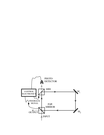
FIG. 2.: Possible experimental setup for single photon extraction by adaptive absorption.

In this scheme only four optical elements and a single photodetector are needed. When a light pulse is trapped in the loop enclosed between the modulated beam splitter $MBS$, the mirrors $M_{1}$ and $M_{2}$, and the flip mirror, it is effectively coupled to the environment through the modulated beam splitter $MBS$. The value of its reflectivity is set close to one and can be slightly increased via an electric current to make it fully reflective. In order to effectively feed the initial state into the loop the flip mirror has to open.

The photodetector keeps track of the photon losses and as soon as it fires, it sends a feedback signal to the flip-mirror so that the pulse can exit the loop without any further losses. Alternatively, the coupling of the field to the environment can be switched off by turning the $MBS$ fully reflective. The flip mirror is then switched whenever the output is desired. This last alternative allows the system to provide the unconditioned evolved states. Otherwise different sub-ensembles will emerge at the output at different times. Depending on the response times of the photodetector, control electronics, modulated beam-splitter, and the flip-mirror one can add a delay line within the loop, for example between the two mirrors $M_{1}$ and $M_{2}$.

Any real experiment will inevitably be only an approximation to the model described above. In practice every beam splitter has a finite reflectivity and has some internal losses, and detectors have efficiencies below one. Inclusion of such effects will degrade the performance of the device.

V Properties of the evolved state

In this section we list some properties of the evolved state. Eqs. (14) and (15) give the conditional and unconditional evolution for an arbitrary initial state and we now present the evolution for two important examples.

A Coherent state

We consider first the important example of an initial coherent state $\rho^{\alpha}(0)=\left|\alpha\right>\!\!\left<\alpha\right|$. As shown in Eq. (11), a coherent state remains unaffected under the action of the jump superoperator $\hat{J}$. This can be understood in the context of the implementation in Fig. 2. As already mentioned, coherent states have the peculiarity that when sent through a beam splitter the two outcoming beams are not entangled. This implies that the transmitted beam is the same independently of the measurement outcome at the photodetector. In any case, while coupled to the environment, the coherent amplitude is damped following Eq. (13). Thus the output field is determined only by the time which the states spend in contact with the environment (inside the loop in Fig. 2), that is the time until the first jump occurs. The conditioned state at the output when the detector fires at $t_{1}$ is given by

$$\rho_{c}^{\alpha}(t)=\left|\alpha\mbox{e}^{-\Gamma t_{1}}\right>\!\!\left<\alpha\mbox{e}^{-\Gamma t_{1}}\right|\mbox{.}$$ (18)

This occurs with the probability

$$p(t_{1}|\alpha)\mbox{d}t=2\Gamma|\alpha|^{2}\mbox{e}^{-2\Gamma t_{1}}\exp[-|\alpha|^{2}(1-\mbox{e}^{-2\Gamma t_{1}})]\mbox{d}t\mbox{.}$$ (19)

Following Eq. (15) the unconditional evolution of the coherent state is

$$\rho^{\alpha}(t) = \exp[-|\alpha|^{2}(1-\mbox{e}^{-2\Gamma t})]\left|\alpha\mbox{e}^{-\Gamma t}\right>\!\!\left<\alpha\mbox{e}^{-\Gamma t}\right|$$ (20)

$$+ \int_{0}^{t}\mbox{d}t_{1}2\Gamma|\alpha|^{2}\mbox{e}^{-2\Gamma t_{1}}$$ (22)

$$\times\exp[-|\alpha|^{2}(1-\mbox{e}^{-2\Gamma t_{1}})]\left|\alpha\mbox{e}^{-\Gamma t_{1}}\right>\!\!\left<\alpha\mbox{e}^{-\Gamma t_{1}}\right|\mbox{.}$$

The P-representation of this state, defined by the equation

$$\rho^{\alpha}(t)=\int\mbox{d}^{2}\beta P^{\alpha}(\beta,t)\left|\beta\right>\!\!\left<\beta\right|\mbox{,}$$ (23)

is given by

$$P^{\alpha}(\beta,t)=\left\{\exp[-|\alpha|^{2}(1-\mbox{e}^{-2\Gamma t})]|\beta|^{-1}\right.$$ (24)

$$\times \left.\delta(|\beta|-|\alpha|\mbox{e}^{-\Gamma t})+2\mbox{e}^{(|\beta|^{2}-|\alpha|^{2})}H(|\beta|-|\alpha|\mbox{e}^{-\Gamma t})\right.$$ (25)

$$\times \left.H(|\alpha|-|\beta|)\right\}\delta(\arg\alpha-\arg\beta)\mbox{,}$$ (26)

where $H(x)$ is the Heaviside step function. The existence and form of this P-function allow us to draw some conclusions: 1) The state produced in this way will have essentially classical properties. 2) The removal of the photon does not change the argument of the coherent state in that the P-function is zero for phases other than $\arg\alpha$.

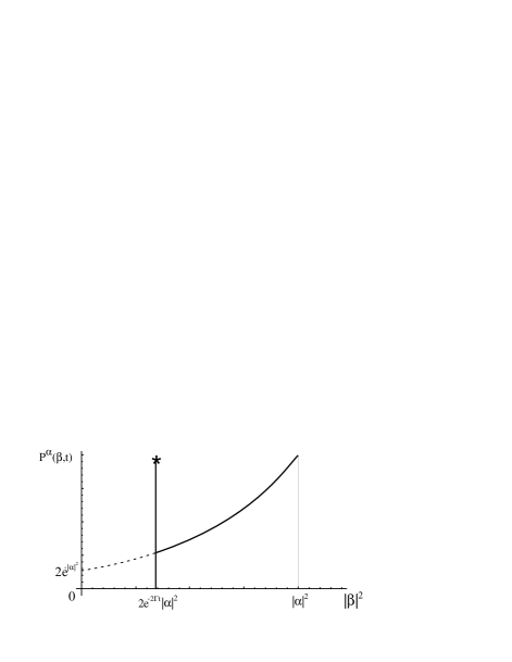
FIG. 3.: P-distribution for a coherent state $\left|\alpha\right>$ evolved until time $t$ (full line). $P^{\alpha}(\beta,t)$ is non-vanishing only at the fixed phase $\arg\beta=\arg\alpha$.

The plot of the P-function $P^{\alpha}(\beta,t)$ in Fig. 3 gives us an intuitive picture of the evolution of the unconditioned state. The initial state $\left|\alpha\right>$ transforms after a time $t$ into a mixture of coherent states with damped amplitudes $|\beta|\in[|\alpha|\mbox{e}^{-\Gamma t},|\alpha|)$. The contribution in the mixture of each coherent state also decays exponentially. The singular peak ($*$ in Fig. 3) corresponds to the case where the detector has not fired, and it takes the required weight to keep $P^{\alpha}(\beta,t)$ normalized.

B Number states and photon statistics

Another important basis-state is the number state $\left|n\right>$. With probability

$$p(t_{1}|n)\mbox{d}t=2\Gamma n\mbox{e}^{-2\Gamma nt_{1}}\mbox{d}t$$ (27)

the number state $\left|n\right>$ will lose one photon at time $t_{1}$, to produce the conditioned state

$$\rho_{c}^{n}(t)=\left|n-1\right>\!\!\left<n-1\right|$$ (28)

for times $t>t_{1}$. This state is independent of the time $t_{1}$ in which the jump occurs. As a result, the unconditioned state when no information on the detection events is available, reduces to the simple form,

$$\rho^{n}(t)=\mbox{e}^{-2n\Gamma t}\left|n\right>\!\!\left<n\right|+(1-\mbox{e}^{-2n\Gamma t})\left|n-1\right>\!\!\left<n-1\right|\mbox{.}$$ (29)

In contrast to the coherent state case, the number state soon evolves into a pure state. The probability of not extracting one photon from $\left|n\right>$ falls exponentially with time, thus the extraction is bound to occur given enough time. After long times $t\rightarrow\infty$ a single photon is removed from the signal deterministically (unless, of course, there was no photon to begin with).

This last remarks are in fact valid for any initial state $\rho(0)=\sum_{n,n^{\prime}=0}^{\infty}\rho_{n,n^{\prime}}\left|n\right>\!\!\left<n^{\prime}\right|$. Indeed, the photon number probability distribution at a time $t$ is given by

$$p_{n}(t) = \left<n\right|\rho(t)\left|n\right>$$ (30)

$$= \mbox{e}^{-2n\Gamma t}p_{n}(0)+(1-\mbox{e}^{-2n\Gamma t})p_{n+1}(0).$$ (31)

And for $t\rightarrow\infty$ we have

$$p_{n}(\infty)=p_{n+1}(0)+p_{0}(0)\delta_{n,0}$$ (32)

which means that the probability distribution is shifted one step to smaller values of $n$. The initial vacuum component is of course not shifted and still receives the contribution from the initial one-photon component. In this limit of large times the mean and variance of the photon number can be easily calculated using Eq. (32),

$$\bar{n}(\infty) = \bar{n}(0)+p_{0}(0)-1\mbox{,}$$ (33)

$$\Delta n^{2}(\infty) = \Delta n^{2}(0)-p_{0}(0)[2\bar{n}(0)+p_{0}(0)-1]$$ (34)

$$= \Delta n^{2}(0)-p_{0}(0)[\bar{n}(0)+\bar{n}(\infty)]\mbox{.}$$ (35)

The mean photon number decreases by an amount equal to the initial probability of having a non-vacuum signal. The variance decreases by an amount dictated by the vacuum probability and also by the mean photon number. From the results in the previous section we know that adaptive absorption cannot produce non-classical light from initially classical light, in the sense that it preserves the positivity of the P-function. Despite this, it still enables us to change substantially the photon statistics of the incoming field. The normally ordered variance of the number operator is

$$:\!\Delta n^{2}\!:(\infty) = \Delta n^{2}(\infty)-\bar{n}(\infty)$$ (36)

$$= :\!\Delta n^{2}\!:(0)+1-p_{0}(0)[2\bar{n}(0)+p_{0}(0)]\mbox{.}$$ (37)

It is now easy to find an example in which an initial super-Poissonian distribution ($:\!\Delta n^{2}\!:>0$) gives a sub-Poissonian output field. An incoming field $\rho^{A}(0)$ with $p^{A}_{n}(0)=p_{0}\delta_{n,0}+(1-p_{0})\delta_{n,N}$ has a normal ordered variance $:\!\Delta n^{2}\!:=N(1-p_{0})(Np_{0}-1)$ which is positive for $N>p_{0}^{-1}$. After long times the corresponding output field will have the normal ordered variance,

$$:\!\Delta n^{2}\!:^{A}(\infty)=(N-1)(1-p_{0})[(N-1)p_{0}-1]\mbox{,}$$ (38)

which becomes negative for $1<N<p_{0}^{-1}+1$. Summarizing, for every non-integer value of $p_{0}^{-1}$ there exists an integer $N$ which fulfills the inequalities $p_{0}^{-1}<N<p_{0}^{-1}+1$ so that the corresponding super-Poissonian input field becomes sub-Poissonian after the adaptive absorption procedure.

VI Adaptive absorption as photon number measurement

Along the course of this paper we have investigated adaptive absorption as a way to manipulate photonic states. By now we have expressed in many ways the idea that the induced evolution is non-unitary and that the coupling to the environment plays a crucial role in this manipulation. In quantum information theory this type of evolution is always accompanied by an outflow of information to the environment. In this section we show that indeed adaptive absorption can also be understood as a procedure to measure the input photonic state. The balance between information gain and disturbance is highly non-trivial and delicate. Moreover, when the system under study is an optical field-mode we find practical limitations in that many of the interesting quantum operations require non-linear optical devices. Here we present a potentially valuable tool which only makes use of linear optical elements.

In Section V B we have seen that for long times, the effect of adaptive absorption on the photon number distribution was to shift it down by one. Now we will see that by keeping track of the detection times $t_{1}$ we can obtain information on the initial photon-number. Taking into account that the probability of removing one photon from a state of $n$ photons is the same as for the analogous classical problem, it is easy to understand that the larger the initial photon number, the easier (i.e., the faster) it is to extract a single photon. The time $t_{1}$ at which the photon is absorbed is our measurement outcome. In fact, at each time step we are effectively performing the measurement defined by the positive operator-valued measure or POVM [19] $\{\Pi_{1}=2\mbox{d}t\Gamma a^{\dagger}a,\Pi_{0}=\openone-\Pi_{1}\}$. Since the absorption POVM $\Pi_{1}$ is infinitesimally small, most of the times we get the “0” outcome. The value of $t_{1}$ conveys the result of the measurements up to $t_{1}$. In order to know the information obtained from the knowledge of $t_{1}$, the central quantity is the probability $p(n|t_{a})$ of having a certain number $n$ of photons in the input given that the measurement outcome is $t_{1}=t_{a}$. By invoking Bayes theorem we can write this conditional probability as

$$p(n|t_{a})=\frac{p(t_{a}|n)p_{n}}{p(t_{a})}=\frac{p(t_{a}|n)}{\sum_{m=1}^{\infty}p(t_{a}|n)}\mbox{,}$$ (39)

where $p(t_{a})=\sum_{n=0}^{\infty}p_{n}p(t_{a}|n)$ and we assume for definiteness a flat a priori probability distribution $p_{n}=p$ $\forall n$. Use of the conditional probability given in Eq. (27) gives

$$p(n|t_{a})=n\mbox{e}^{-2\Gamma(n+1)t_{a}}(\mbox{e}^{2\Gamma t_{a}}-1)^{2}\mbox{.}$$ (40)

We note that summation of this expression over $n$ from $1$ to $\infty$ gives unity as it should. The exponential dependence on $n$ may provide the means to discriminate between states with widely differing photon numbers without detecting all of the photons (see Figure 4). The technique cannot, of course, determine the number of photons without error. The benefit of this technique as a measurement, however, is likely to be in those situations where we can only afford to weakly perturb the mode. A possible application of this idea to quantum cryptography is discussed briefly in the concluding section.

FIG. 4.: $p(n|t_{a})$ for $\Gamma=1$ and three different values of $n=\{1,2,5\}$.

VII Conclusions

In this paper we have presented the idea of extracting a single photon from an arbitrary single-mode field via adaptive absorption. The extraction of a single photon can also be achieved by post-selection, that is by setting up a beam splitter and considering at the end only those situations in which a single photon was removed. Of course this is not deterministic and would in fact lead to the possibility of removing more than one photon. The fact that one can stop the absorption process as soon as one photon is absorbed is the novel aspect of this work. For example this possibility has given rise to a novel eavesdropping attack on quantum key distribution (QKD) [20]. There are two factors that might render insecure many of the current implementations of QKD [21]: the signals are weak coherent pulses instead of single photons and the communication channels have very high losses. The eavesdropper can acquire the secret key whenever he succeeds in extracting a single photon from the multiphoton part of the signal. Adaptive absorption allows the eavesdropper to take advantage of this security gap by using current technology.

By repeatedly applying the single-photon extraction one can extract any number of photons in a controlled way. Moreover, as we have seen in the previous section, in process of extracting single-photons we also obtain information on the input system. Thus adaptive absorption implements weak measurements, where the measured system is only slightly disturbed.

Adaptive absorption is a simple example of a general idea that can give rise to many other applications. Another example, that falls outside the scope of this paper, is adaptive amplification as a means to add a single excitation into a mode. This general idea is to use the results of a continuous measurement to modify the system Hamiltonian or its coupling to the measurement apparatus. This line of action may lead to novel quantum operations or ease the realization of operations with too high technological demands.

VIII Acknowledgements

S. M. B. thanks the Royal Society of Edinburgh and the Scottish Executive Education and Lifelong Learning Department for financial support. J.C. and K-A.S. acknowledge the Academy of Finland (project 4336) and the European Union IST EQUIP Programme for financial support.

REFERENCES

- [1] Y. Yamamoto, N. Imoto and S. Machida, Phys. Rev. A 33, 3243 (1986).
- [2] J.M. Shapiro et al., J. Opt. Soc. Am. B 4, 1604 (1987).
- [3] H.M. Wiseman and G.J. Milburn, Phys. Rev. Lett. 70, 548 (1993); H.M. Wiseman, Phys. Rev. A 49, 2133 (1994); 49, 5159(E) (1994); 50, 4428(E) (1994).
- [4] A. C. Doherty and K. Jacobs, Phys. Rev. A 60, 2700 (1999).
- [5] A. C. Doherty et al., Phys. Rev. A 62, 12105 (2000).
- [6] J.A. Dunningham, H.M. Wiseman, and D.F. Walls, Phys. Rev. A 55, 1398 (1997).
- [7] S. Mancini, D. Vitali, and P. Tombesi, Phys. Rev. Lett. 80, 688 (1998).
- [8] H.F. Hofmann, G. Mahler, and O. Hess, Phys. Rev. A 57, 4877 (1998).
- [9] H. Mabuchi and P. Zoller, Phys. Rev. Lett. 76, 3108 (1996).
- [10] H.M. Wiseman, Phys. Rev. Lett. 81, 3840 (1998).
- [11] P. Tombesi and D. Vitali, Appl. Phys. B. 60, S69 (1995).
- [12] P. Goetsch, P. Tombesi and D. Vitali, Phys. Rev. A 54, 4519 (1996); D. B. Horoshko and S. Ya. Kilin, Phys. Rev. Lett. 78, 840 (1997).
- [13] E. Knill, R. Laflamme, and G. Milburn, Nature 409, 46 (2001); D. Bouwmeester, Phys. Rev. A 63, R040301 (2001); J.-W. Pan et al, Nature 410, 1067 (2001); D. Bouwmeester et al., Nature 390, 575 (1997); S. L. Braunstein and H. J. Kimble, Phys. Rev. Lett. 80, 869 (1998); H. Weinfurter, Europhys. Lett. 25, 559 (1994); S. L. Braunstein and A. Mann, Phys. Rev. A 51, R1727 (1995); M. Michler, K. Mattle, H. Weinfurter, and A. Zeilinger, Phys. Rev. A 53, R1209 (1996); J. Calsamiglia and N. Lütkenhaus, Appl. Phys. B 72, 67 (2001).
- [14] U. Leonhardt, Phys. Rev. A 48, 3265 (1993).
- [15] M. S. Kim and N. Imoto, Phys. Rev. A 52, 2401 (1995).
- [16] R. A. Campos, B. E. A. Saleh, and M. C. Teich, Phys. Rev. A 40, 1371 (1989).
- [17] S. M. Barnett and P. M. Radmore, Methods in theoretical quantum optics (Clarendon Press, Oxford, 1997).
- [18] H. Carmichael, An open system approach to quantum optics (Springer-Verlag, Berlin, 1993).
- [19] A. Peres, Quantum Theory: Concepts and Methods (Kluwer, Dordrecht, 1993); C. W. Helstrom, Quantum Detection and Estimation Theory (Academic Press, New York, 1976).
- [20] J. Calsamiglia, S.M. Barnett and N. Lütkenhaus, in preparation.
- [21] B. Huttner, N. Imoto, N. Gisin, and T. Mor Phys. Rev. A 51, 1863 (1995).