Quantum memory for photons: I. Dark state polaritons

Abstract

An ideal and reversible transfer technique for the quantum state between light and metastable collective states of matter is presented and analyzed in detail. The method is based on the control of photon propagation in coherently driven 3-level atomic media, in which the group velocity is adiabatically reduced to zero. Form-stable coupled excitations of light and matter (“dark-state polaritons”) associated with the propagation of quantum fields in Electromagnetically Induced Transparency are identified, their basic properties discussed and their application for quantum memories for light analyzed.

I introduction

Recent advances in quantum information science lead to many interesting new concepts such as quantum computation, quantum cryptography and teleportation [1, 2, 3]. The practical implementation of quantum processing protocols requires coherent manipulation of a large number of coupled quantum systems which is an extremely difficult task. One of the particular challenges for the implementation of these ideas involves physically transporting or communicating quantum states between different nodes of quantum networks [4]. Quantum optical systems appear to be very attractive for the realization of such networks. On one hand photons are ideal carriers of quantum information: they are fast, robust and readily available. On the other hand atoms represent reliable and long-lived storage and processing units. Therefore the challenge is to develop a technique for coherent transfer of quantum information carried by light to atoms and vise versa. In other words it is necessary to have a quantum memory that is capable of storing and releasing quantum states on the level of individual qubits and on demand. Such a device needs to be entirely coherent and in order to achieve a unidirectional transfer (from field to atoms or vise versa) an explicit time dependent control mechanism is required.

Classical optical data storage in the time domain, based on the phenomenon of spin- [5] and photon echo [6], has a long history. After the first proposals of stimulated two-level photon echo [7] and demonstrations of light-pulse storage in these systems [8] many important developments have taken place in this field. Particularly interesting are techniques based on Raman photon echos [9] as they combine the long livetime of ground-state hyperfine or Zeeman coherences for storage with data transfer by light at optical frequencies [10]. While these techniques are very powerful for high-capacity storage of classical optical data, they cannot be used for quantum memory purposes. The techniques employ direct or dressed-state optical pumping and thus contain dissipative elements or have other limitations in the transfer process between light and matter. As a consequence they do not operate on the level of individual photons and cannot be applied for quantum information processing.

The conceptually simplest approach to a quantum memory for light is to “store” the state of a single photon in an individual atom. This approach involves a coherent absorption and emission of single photons by single atoms. However, the single-atom absorption cross-section is very small, which makes such a process very inefficient. A very elegant solution to this problem is provided by cavity QED [11]. Placing an atom in a high-$Q$ resonator effectively enhances its cross-section by the number of photon round-trips during the ring-down time and thus makes an effective transfer possible. Raman adiabatic passage techniques [12] with time-dependent external control fields can be used to implement a directed but reversible transfer of the quantum state of a photon to the atom (i.e. coherent absorption). However, despite the enormous experimental progress in this field [13], it is technically very challenging to achieve the necessary strong-coupling regime. Furthermore the single-atom system is by construction highly susceptible to the loss of atoms and the speed of operations is limited by the large $Q$-factor.

On the other hand a photon can be absorbed with unit probability in an optically thick ensemble of atoms. Normally such absorption is accompanied by dissipative processes which result in decoherence and thus deteriorate the quantum state. Nevertheless it has been shown that such absorption of light leads to a partial mapping of its quantum properties to atomic ensembles [14, 15]. As a consequence of dissipation these methods do not allow to reversibly store the quantum state on the level of individual photon wave-packets (single qubits). Rather a stationary source of identical copies is required (e.g. a stationary source of squeezed vacuum, which can be considered as a train of identical wave-packets in a squeezed vacuum state) to partially map quantum statistics from light to matter.

Recently we have proposed a method that combines the enhancement of the absorption cross section in many-atom systems with dissipation-free adiabatic passage techniques [16, 17, 18]. It is based on an adiabatic transfer of the quantum state of photons to collective atomic excitations using electromagnetically induced transparency (EIT) in 3-level atoms [19]. Since the technique alleviates most of the stringent requirements of single-atom cavity-QED, it could become the basis for a fast and reliable quantum network. Recent experiments [20, 21] have already demonstrated one of the basic principle of this technique - the dynamic group velocity reduction and adiabatic following in the so-called “dark-state” polaritons. The aim of the present and subsequent papers is to analyze the physics of the reversible storage technique in detail and to discuss its potentials and limitations.

Electromagnetically induced transparency can be used to make a resonant, opaque medium transparent by means of quantum interference. Associated with the transparency is a large linear dispersion, which has been demonstrated to lead to a substantial reduction of the group velocity of light [22]. Since the group velocity reduction is a linear process, the quantum state of a slowed light pulse can be preserved. Therefore a non-absorbing medium with a slow group velocity is in fact a temporary “storage” device. However, such a system has only limited “storage” capabilities. In particular the achievable ratio of storage time to pulse length is limited by the square root of the medium opacity [23] and can practically attain only values on the order of 10 to 100. This limitation originates from the fact that a small group velocity is associated with a narrow spectral acceptance window of EIT [24] and hence larger delay times require larger initial pulse length.

The physics of the state-preserving slow light propagation in EIT is associated with the existence of quasi-particles, which we call dark-state polaritons (DSP). A dark-state polariton is a mixture of electromagnetic and collective atomic excitations of spin transitions (spin-wave). The mixing angle between the two components determines the propagation velocity and is governed by the atomic density and the strength of an external control field. The key idea of the present approach is the dynamic rotation of the mixing angle which leads to an adiabatic passage from a pure photon-like to a pure spin-wave polariton thereby decelerating the initial photon wavepacket to a full stop. In this process the quantum state of the optical field is completely transferred to the atoms. During the adiabatic slowing the spectrum of the pulse becomes narrower in proportion to the group velocity, which essentially eliminates the limitations on initial spectral width or pulse length and very large ratios of storage time to initial pulse length can be achieved. Reversing the rotation at a later time regenerates the photon wave-packet. Hence the extension of EIT to a dynamic group-velocity reduction via adiabatic following in polaritons can be used as the basis of an effective quantum memory. Before proceeding we note some earlier work on the subject. The polariton picture of Raman adiabatic passage has first been introduced in Ref. [25]. Furthermore Grobe and coworkers [26] pointed out that the spatial profile of an atomic Raman coherence can be mirrored into the electromagnetic field by coherent scattering, whereas time-varying fields can be used to create spatially non-homogeneous matter excitations.

In the present paper we will present a quantum picture of slow light propagation in EIT in terms of dark-state polaritons. We will analyze the properties of the polaritons and discuss their application to reversible, fast and high-fidelity quantum memories. Limitations and restrictions of the transfer process from non-adiabatic processes will be discussed as well as effects from the medium boundary and atomic motion. Other important aspects of the collective quantum memory such as its decoherence properties will be the subject of subsequent publications.

II quantum memory for a single-mode field

The essential aspects of the quantum state mapping technique can be most easily understood for the case of a single mode of the radiation field as realized e.g. in a single mode optical cavity. In what follows we will address this case first in order to motivate the following discussion on propagating photon wave packets.

Consider a collection of $N$ 3-level atoms with two meta-stable lower states as shown in Fig. 1 interacting with two single-mode optical fields. The transition $|a\rangle\to|b\rangle$ of each of these atoms is coupled to a quantized radiation mode. Moreover the transitions from $|a\rangle\to|c\rangle$ are resonantly driven by a classical control field of Rabi-frequency $\Omega$. The dynamics of this system is described by the interaction Hamiltonian:

$$H=\hbar g\sum_{i=1}^{N}\hat{a}\sigma_{ab}^{i}+\hbar\Omega(t){\rm e}^{-i\nu t}\sum_{i=1}^{N}\sigma_{ac}^{i}+{\rm h.c.}.$$ (1)

Here $\sigma_{\mu\nu}^{i}=|\mu\rangle_{ii}\langle\nu|$ is the flip operator of the $i$th atom between states $|\mu\rangle$ and $|\nu\rangle$. $g$ is the coupling constant between the atoms and the quantized field mode (vacuum Rabi-frequency) which for simplicity is assumed to be equal for all atoms.

When all atoms are prepared initially in level $|b\rangle$ the only states coupled by the interaction are the totally symmetric Dicke-like states [27]

$$|{\bf b}\rangle = |b_{1},b_{2},\dots,b_{N}\rangle,$$ (2)

$$|{\bf a}\rangle = \frac{1}{\sqrt{N}}\sum_{j=1}^{N}|b_{1},\dots,a_{j},\dots,b_{N}\rangle,$$ (3)

$$|{\bf c}\rangle = \frac{1}{\sqrt{N}}\sum_{j=1}^{N}|b_{1},\dots,c_{j},\dots,b_{N}\rangle,$$ (4)

$$|{\bf aa}\rangle = \frac{1}{\sqrt{2N(N-1)}}\sum_{i\neq j=1}^{N}|b_{1},\dots,a_{i},\dots,a_{j},\dots,b_{N}\rangle$$ (6)

$${\rm etc.}$$

In particular, if the field is initially in a state with at most one photon, the relevant eigenstates of the bare system are: the total ground state $|{\bf b},0\rangle$, which is not affected by the interaction at all, the ground state with one photon in the field $|{\bf b},1\rangle$, as well as the singly excited states $|{\bf a},0\rangle$ and $|{\bf c},0\rangle$. For the case of two excitations, the interaction involves 3 more states etc. The coupling of the singly and doubly excited systems are shown in Fig. 1 b.

FIG. 1.: a) 3-level atoms coupled to single quantized mode and classical control field of (real) Rabi-frequency $\Omega(t)$. b) coupling of relevant bare eigenstates for at most one photon

The interaction has families of dark-states, i.e. states with zero adiabatic eigenvalue [11, 16, 18]. The simplest one is

$$|D,1\rangle = \cos\theta(t)\,|{\bf b},1\rangle-\sin\theta(t)\,|{\bf c},0\rangle,$$ (8)

$$\tan\theta(t)=\frac{g\sqrt{N}}{\Omega(t)},$$

and in general one has

$$|D,n\rangle=$$ (9)

$$\enspace=\sum_{k=0}^{n}\sqrt{\frac{n!}{k!(n-k)!}}(-\sin\theta)^{k}(\cos\theta)^{n-k}|{\bf c}^{k},n-k\rangle.$$ (10)

The dark states do not contain the excited state and are thus immune to spontaneous emission. It should also be noted that although the dark states $|D,n\rangle$ are degenerate they belong to exactly decoupled subsystems as long as spontaneous emission is disregarded. This means there is no transition between them even if non-adiabatic corrections are taken into account. The existence of collective dark states provides a very elegant way to transfer the quantum state of the single-mode field to collective atomic excitations. Adiabatically rotating the mixing angle $\theta$ from $0$ to $\pi/2$ leads to a complete and reversible transfer of the photonic state to a collective atomic state if the total number of excitations $n$ is less than the number of atoms. This can be seen very easily from the expression for the dark states, eq.(10): If $\theta:0\to\pi/2$ one has for all $n\leq N$

$$|D,n\rangle:\,|{\bf b}\rangle|n\rangle\longrightarrow|{\bf c}^{n}\rangle|0\rangle.$$ (11)

Thus if the initial quantum state of the single-mode light field is in any mixed state described by a density matrix $\hat{\rho}_{f}=\sum_{n,m}\rho_{nm}\,|n\rangle\langle m|$, the transfer process generates a quantum state of collective excitations according to

$$\sum_{n,m}\rho_{nm}\,|n\rangle\langle m|\otimes|{\bf b}\rangle\langle{\bf b}|\longrightarrow$$ (12)

$$\qquad\qquad|0\rangle\langle 0|\otimes\sum_{n,m}\rho_{nm}\,|{\bf c}^{n}\rangle\langle{\bf c}^{m}|.$$ (13)

It should be noted that the quantum-state transfer does not necessarily constitute a transfer of energy from the quantum field to the atomic ensemble. Since in the Raman process the coherent “absorption” of a photon from the quantized mode is followed by a stimulated emission into the classical control field, most of the energy is actually deposited in the latter field.

The transfer of quantum states between light and matter due to adiabatic following in collective dark states is the key point of the present work. Before proceeding we also note that the transfer rate is proportional to the total number of atoms $N$, which is a signature of collective coupling. This makes the proposed method potentially fast and robust.

III quantum description of slow-light propagation

We now discuss a generalization of the mapping technique to propagating fields. The adiabatic transfer of the quantum state from the radiation mode to collective atomic excitations discussed in the previous section is strongly related to intracavity electromagnetically induced transparency (EIT) [28]. In order to generalize the technique to multi-mode fields it is useful to discuss first the propagation of light in 3-level media under conditions of EIT.

A model

Consider the quasi 1-dimensional problem shown in Fig. 2. A quantized electromagnetic field with positive frequency part of the electric component $\hat{E}^{(+)}$ couples resonantly the transition between the ground state $|b\rangle$ and the excited state $|a\rangle$. $\nu=\omega_{ab}$ is the carrier frequency of the optical field. The upper level $|a\rangle$ is furthermore coupled to the stable state $|c\rangle$ via a coherent control field with Rabi-frequency $\Omega$.

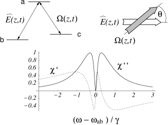
FIG. 2.: top: 3-level $\Lambda$-type medium resonantly coupled to a classical field with Rabi-frequency $\Omega(t)$ and quantum field $\hat{E}(z,t)$. bottom: Typical susceptibility spectrum for probe field $\hat{E}$ as function of normalized detuning from resonance for resonant drive field. Real part $\chi^{\prime}$ describes refractive index contribution and imaginary part $\chi^{\prime\prime}$ absorption.

The interaction Hamiltonian reads

$$\hat{V} = -\wp\sum_{j}\Bigl{(}\hat{\sigma}_{ab}^{j}\,\hat{E}^{(+)}(z_{j})+h.a\Bigr{)}$$ (15)

$$-\hbar\sum_{j}\Bigl{(}\hat{\sigma}_{ac}^{j}\,\Omega(z_{j},t)\,{\rm e}^{i(k_{d}^{\parallel}z_{j}-\nu_{d}t)}+h.a\Bigr{)}$$

where $z_{j}$ denotes the position of the $j$th atom, $\wp$ denotes the dipole matrix element between the states $|a\rangle$ and $|b\rangle$, and

$$\hat{\sigma}_{\alpha\beta}^{j}\equiv|\alpha_{j}\rangle\langle\beta_{j}|$$ (16)

defines the atomic flip operators. $k_{d}^{\parallel}=\vec{k}_{d}\cdot\vec{\rm e}_{z}=\frac{\nu_{d}}{c}\cos\vartheta$ is the projection of the wavevector of the control field to the propagation axis of the quantum field. For the sake of simplicity we here assume that the carrier frequencies $\nu$ and $\nu_{d}$ of the quantum and control fields coincide with the atomic resonances $\omega_{ab}$ and $\omega_{ac}$ respectively. Motional effects and the associated Doppler-shifts will be discussed later. We introduce slowly-varying variables according to

$$\hat{E}^{(+)}(z,t) = \sqrt{\frac{\hbar\nu}{2\varepsilon_{0}V}}\hat{\cal E}(z,t)\,{\rm e}^{i\frac{\nu}{c}(z-ct)},$$ (17)

$$\hat{\sigma}_{\mu\nu}^{j}(t) = {\widetilde{\sigma}}_{\mu\nu}^{j}(t)\,{\rm e}^{-i\frac{\omega_{\mu\nu}}{c}(z-ct)}.$$ (18)

Here $V$ is some quantization volume, which for simplicity was chosen to be equal to the interaction volume.

If the (slowly-varying) quantum amplitude does not change in a length interval $\Delta z$ which contains $N_{z}\gg 1$ atoms we can introduce continuum atomic variables

$${\widetilde{\sigma}}_{\mu\nu}(z,t)=\frac{1}{N_{z}}\sum_{z_{j}\in N_{z}}\,{\widetilde{\sigma}}_{\mu\nu}^{j}(t)$$ (19)

and make the replacement $\sum_{j=1}^{N}\longrightarrow\frac{N}{L}\int{\rm d}z$, where $N$ is the number of atoms, and $L$ the length of the interaction volume in propagation direction of the quantized field. This yields the continuous form of the interaction Hamiltonian

$${\hat{V}} = -\int\!\!\frac{{\rm d}z}{L}\biggl{(}\hbar gN{\widetilde{\sigma}}_{ab}(z,t)\,\hat{\cal E}(z,t)$$ (21)

$$\qquad\qquad+\hbar\Omega(z,t){\rm e}^{i\Delta kz}N(z){\widetilde{\sigma}}_{ac}(z,t)+h.a.\biggr{)}.$$

Here $g=\wp\sqrt{\frac{\nu}{2\hbar\epsilon_{0}V}}$ is the atom-field coupling constant and $\Delta k=k_{d}^{\parallel}-k_{d}=\frac{\omega_{ac}}{c}\left(\cos\vartheta-1\right)$.

The evolution of the Heisenberg operator corresponding to the quantum field can be described in slowly varying amplitude approximation by the propagation equation

$$\left(\frac{\partial}{\partial t}+c\frac{\partial}{\partial z}\right)\hat{\cal E}(z,t)={i}gN\,{\widetilde{\sigma}}_{ba}(z,t).$$ (22)

The atomic evolution is governed by a set of Heisenberg-Langevin equations

$$\dot{\widetilde{\sigma}}_{aa} = -\gamma_{a}{\widetilde{\sigma}}_{aa}-ig\Bigl{(}\hat{\cal E}^{\dagger}{\widetilde{\sigma}}_{ba}-h.a.\Bigr{)}$$ (24)

$$-i\Bigl{(}\Omega^{*}{\rm e}^{-i\Delta kz}{\widetilde{\sigma}}_{ca}-h.a\Bigr{)}+F_{a},$$

$$\dot{\widetilde{\sigma}}_{bb} = \gamma{\widetilde{\sigma}}_{aa}+ig\Bigl{(}\hat{\cal E}^{\dagger}{\widetilde{\sigma}}_{ba}-h.a.\Bigr{)}+F_{b},$$ (25)

$$\dot{\widetilde{\sigma}}_{cc} = \gamma^{\prime}{\widetilde{\sigma}}_{aa}+i\Bigl{(}\Omega^{*}{\rm e}^{-i\Delta kz}{\widetilde{\sigma}}_{ca}-h.a\Bigr{)}+F_{c},$$ (26)

$$\dot{\widetilde{\sigma}}_{ba} = -\gamma_{ba}{\widetilde{\sigma}}_{ba}+ig{\cal E}\Bigl{(}{\widetilde{\sigma}}_{bb}-{\widetilde{\sigma}}_{aa}\Bigr{)}$$ (28)

$$+i\Omega{\rm e}^{i\Delta kz}{\widetilde{\sigma}}_{bc}+F_{ba},$$

$$\dot{\widetilde{\sigma}}_{ca} = -\gamma_{ca}{\widetilde{\sigma}}_{ca}+i\Omega{\rm e}^{i\Delta kz}\Bigl{(}{\widetilde{\sigma}}_{cc}-{\widetilde{\sigma}}_{aa}\Bigr{)}$$ (30)

$$+ig\hat{\cal E}{\widetilde{\sigma}}_{ba}+F_{ca},$$

$$\dot{\widetilde{\sigma}}_{bc} = i\Omega^{*}{\rm e}^{-i\Delta kz}{\widetilde{\sigma}}_{ba}-ig\hat{\cal E}{\widetilde{\sigma}}_{ac},$$ (31)

$\gamma_{a}=\gamma+\gamma^{\prime}$ and $\gamma,\gamma^{\prime}$ denote longitudinal and $\gamma_{\mu\nu}$ transversal decay rates. $F_{\mu}$ and $F_{\mu\nu}$ are $\delta$-correlated Langevin noise operators, whose explicit form is not of interest here.

It should be noted that we have disregarded dissipative population exchange processes due to e.g. spin-flip collisions and dephasing of the lower-level transition. This is justified since we assume that the interaction time is sufficiently short compared to the characteristic times of these processes. Both, dissipative population exchange as well as dephasing will be discussed in detail later on.

B low-intensity approximation

In order to solve the propagation problem, we now assume that the Rabi-frequency of the quantum field is much smaller than $\Omega$ and that the number density of photons in the input pulse is much less than the number density of atoms. In such a case the atomic equations can be treated perturbatively in $\hat{\cal E}$. In zeroth order only ${\widetilde{\sigma}}_{bb}={\bf 1}$ is different from zero and in first order one finds

$${\widetilde{\sigma}}_{ba}=-\frac{i}{\Omega^{*}}{\rm e}^{i\Delta kz}\frac{\partial}{\partial t}{\widetilde{\sigma}}_{bc}.$$ (32)

With this the interaction of the probe pulse with the medium can be described by the amplitude of the probe electric field $\hat{\cal E}$ and the collective ground-state spin variable ${\widetilde{\sigma}}_{bc}$:

$$\left(\frac{\partial}{\partial t}+c\frac{\partial}{\partial z}\right)\hat{\cal E}(z,t)=\frac{gN}{\Omega^{*}}{\rm e}^{i\Delta kz}\frac{\partial}{\partial t}{\widetilde{\sigma}}_{bc},$$ (33)

and

$${\widetilde{\sigma}}_{bc}=-\frac{g\hat{\cal E}}{\Omega}{\rm e}^{-i\Delta kz}$$ (34)

$$\enspace-\frac{i}{\Omega}\left[\left(\frac{\partial}{\partial t}+\gamma_{ba}\right)\left(-\frac{i}{\Omega^{*}}\frac{\partial}{\partial t}{\widetilde{\sigma}}_{bc}\right)+{\rm e}^{-i\Delta kz}F_{ba}\right].$$ (35)

C adiabatic limit

The propagation equations simplify considerably if we assume a sufficiently slow change of $\Omega$, i.e. adiabatic conditions [29, 23, 30]. Normalizing the time to a characteristic scale $T$ via $\tilde{t}=t/T$ and expanding the r.h.s. of (35) in powers of $1/T$ we find in lowest non-vanishing order

$${\widetilde{\sigma}}_{bc}(z,t)=-g\frac{\hat{\cal E}}{\Omega}{\rm e}^{-i\Delta kz}.$$ (36)

We note that also the noise operator $F_{ba}$ gives no contribution in the adiabatic limit, since $\langle F_{x}(t)F_{y}(t^{\prime})\rangle\sim\delta(t-t^{\prime})=\delta(\tilde{t}-\tilde{t}^{\prime})/T$. Thus in the perturbative and adiabatic limit the propagation of the quantum light pulse is governed by

$$\left(\frac{\partial}{\partial t}+c\frac{\partial}{\partial z}\right)\hat{\cal E}(z,t) = -\frac{g^{2}N}{\Omega^{*}}\frac{\partial}{\partial t}\frac{\hat{\cal E}(z,t)}{\Omega}.$$ (37)

D slow light and delay-time limitations

If $\Omega(z,t)=\Omega(z)$ is constant in time, the term on the r.h.s. of the propagation equation (37) simply leads to a modification of the group velocity of the quantum field according to

$$v_{g} = v_{g}(z)=\frac{c}{1+n_{g}(z)},$$ (38)

$$n_{g}(z) = \frac{g^{2}N}{|\Omega(z)|^{2}}=\frac{3}{8\pi^{2}}\rho\lambda^{3}\frac{kc\,\gamma}{|\Omega(z)|^{2}},$$ (39)

with $\rho$ being the atom density and $\lambda$ the resonant wavelength of the $a\to b$ transition. The solution of the wave equation is in this case

$$\hat{\cal E}(z,t)=\hat{\cal E}\biggl{(}0,t-\int^{z}_{0}{\rm d}z^{\prime}\,\frac{1}{v_{g}(z^{\prime})}\biggr{)},$$ (40)

where $\hat{\cal E}(0,t^{\prime})$ denotes the field entering the interaction region at $z=0$. This solution describes a propagation with a spatially varying velocity $v_{g}$. It is apparent that the temporal profile of the pulse is unaffected by the slow-down. As a consequence the integrated electromagnetic energy flux through a plane perpendicular to the propagation is the same at any position. Furthermore the spectrum of the pulse remains unchanged

$$S(z,\omega) \equiv \int_{-\infty}^{\infty}\!\!{\rm d}\tau\,{\rm e}^{-i\omega\tau}\,\Bigl{\langle}\hat{\cal E}^{\dagger}(z,t)\hat{\cal E}(z,t-\tau)\Bigr{\rangle}$$ (41)

$$= S(0,\omega).$$ (42)

In particular the spectral width stays constant

$$\Delta\omega_{p}(z)=\Delta\omega_{p}(0).$$ (43)

On the other hand a spatial change of the group velocity, either in a stepwise fashion as e.g. at the entrance of the medium or in a continuous way e.g. due to a spatially decreasing control field, leads to a compression of the spatial pulse profile. In particular, if the group velocity is statically reduced to a value $v_{g}$, the spatial pulse length $\Delta l$ is modified according to

$$\Delta l=\frac{v_{g}}{c}\,\Delta l_{0},,$$ (44)

as compared with a free-space value $\Delta l_{0}$.

It is instructive to discuss the limitations to the achievable delay (and therefore “storage”) time $\tau_{d}$ in an EIT medium with a very small but finite group velocity. A first and obvious limitation is set by the finite lifetime of the dark state, which had been neglected in the previous subsection. If $\gamma_{bc}$ denotes the dephasing rate of the $b-c$ transition it is required that $\tau_{d}\leq\gamma_{bc}^{-1}$. A much stronger limitation arises however from the violation of the adiabatic approximation.

The EIT medium behaves like a non-absorbing, linear dispersive medium only within a certain frequency window around the two-photon resonance (see Fig.2 and [24]). The adiabatic approximation made in the last sub-section essentially assumes that everything happens within this frequency window. If the pulse becomes too short, or its spectrum too broad relative to the transparency width, absorption and higher-order dispersion need to be taken into account.

The transparency window is defined by the intensity transmission of the medium. In order to determine its width we consider the susceptibility of an ideal, homogeneous EIT medium with a resonant drive field. Here one has

$$\chi = \frac{n_{g}}{kc}\frac{|\Omega|^{2}\delta}{|\Omega|^{2}-\delta^{2}-i\gamma\delta}$$ (45)

$$\approx \frac{n_{g}}{kc}\left[\delta+i\delta^{2}\frac{\gamma}{|\Omega|^{2}}+{\cal O}(\delta^{3})\right],$$ (46)

where $\delta=\nu-\omega_{ac}$ is the detuning of the probe field. If we assume a homogeneous drive field, we find

$$T(\delta,z) = \exp\Bigl{\{}-kz\,{\rm Im}[\chi]\Bigr{\}}$$ (47)

$$\approx \exp\Bigl{\{}-\delta^{2}/\Delta\omega_{tr}^{2}\Bigr{\}},$$ (48)

with

$$\Delta\omega_{tr}=\left[\frac{c}{\gamma l}\frac{|\Omega|^{2}}{n_{g}}\right]^{1/2}=\frac{|\Omega|^{2}}{\gamma}\frac{1}{\sqrt{\alpha}},$$ (49)

$l$ being the propagation length in the medium and $\alpha\equiv\frac{3}{8\pi^{2}}\rho\lambda^{3}kl$ the opacity in the absence of EIT. One recognizes that the transparency width decreases with increasing group index. It is instructive to express the transparency width in terms of the pulse delay time $\tau_{d}=n_{g}l/c$ for the medium. This yields

$$\Delta\omega_{tr}=\sqrt{\alpha}\,\frac{1}{\tau_{d}}.$$ (50)

Hence large delay times imply a narrow transparency window, which in turn requires a long pulse time. When the group velocity gets too small such that the transparency window becomes smaller than the spectral width of the pulse, the adiabatic condition is violated, and the pulse is absorbed. Hence there is an upper bound for the ratio of achievable delay (storage) time to the initial pulse length of a photon wavepacket

$$\frac{\tau_{d}}{\tau_{p}}\leq\sqrt{\alpha}\quad{\rm and}\quad\tau_{d}\leq\gamma_{bc}^{-1}.$$ (51)

The ratio $\tau_{d}/\tau_{p}$ is the figure of merit for a memory device. The larger this ratio the better suited is the system for a temporal storage.

There is another quantity which is important for the storage capacity, namely the ratio of medium length $L$ to the length $L_{p}$ of an individual pulse inside the medium. Following similar arguments as above one finds that this quantity is also limited by the square root of the opacity

$$\frac{L}{L_{p}}\leq\sqrt{\alpha},$$ (52)

where $n_{g}\gg 1$ was assumed.

In practice, the achievable opacity $\alpha$ of atomic vapor systems is limited to values below $10^{4}$ resulting in upper bounds for the ratio of time delay to pulse length of the order of 100. Thus dense EIT media with ultra-small group velocity are only of limited use as a temporary storage device. The propagation velocity cannot be made zero and non-adiabatic corrections limit the achievable ratio of storage time to the time length of an individual qubit.

It should be mentioned that the narrowing of the EIT transparency window is also a consideration for effects involving freezing light in a moving media [32] and so-called optical black holes based on EIT [33]. In the following we will show, that EIT can nevertheless be used for memory purposes in a very effective way when combined with adiabatic passage techniques.

IV dark-state polaritons

In the previous section we have discussed the propagation of a quantum field in an EIT medium under otherwise stationary conditions, i.e. with a constant or only spatially varying control field. Since under these conditions, the hamiltonian of the system is time-independent, a coherent process that allows for an uni-directional transfer of the quantum state of a photon wavepacket to the atomic ensemble was not possible. We will show now that this limitation can be overcome easily by allowing for a time-dependent control field. This provides an elegant tool to control the propagation of a quantum light pulse. For a spatially homogeneous but time-dependent control field, $\Omega=\Omega(t)$, the propagation problem can be solved in a very instructive way in a quasi-particle picture. In the following we will introduce these quasi-particles, called dark-state polaritons [17, 25] and discuss their properties, applications and limitations.

A definition of dark- and bright-state polaritons

Let us consider the case of a time-dependent, spatially homogeneous and real control field $\Omega=\Omega(t)=\Omega(t)^{*}$. We introduce a rotation in the space of physically relevant variables – the electric field $\hat{\cal E}$ and the atomic spin coherence ${\widetilde{\sigma}}_{bc}$ – defining two new quantum fields $\hat{\Psi}(z,t)$ and $\hat{\Phi}(z,t)$

$$\hat{\Psi} = \cos\theta(t)\,\hat{\cal E}(z,t)-\sin\theta(t)\,\sqrt{N}\,{\widetilde{\sigma}}_{bc}(z,t)\,{\rm e}^{i\Delta kz},$$ (53)

$$\hat{\Phi} = \sin\theta(t)\,\hat{\cal E}(z,t)+\cos\theta(t)\,\sqrt{N}\,{\widetilde{\sigma}}_{bc}(z,t)\,{\rm e}^{i\Delta kz},$$ (54)

with the mixing angle $\theta(t)$ given by

$$\tan^{2}\theta(t)=\frac{g^{2}N}{\Omega^{2}(t)}=n_{\rm g}(t).$$ (55)

$\hat{\Psi}$ and $\hat{\Phi}$ are superpositions of electromagnetic ($\hat{\cal E}$) and collective atomic components ($\sqrt{N}{\widetilde{\sigma}}_{bc}$), whose admixture can be controlled through $\theta(t)$ by changing the strength of the external driving field.

Introducing a plain-wave decomposition $\hat{\Psi}(z,t)=\sum_{k}\hat{\Psi}_{k}(t)\,{\rm e}^{ikz}$ and $\hat{\Phi}(z,t)=\sum_{k}\hat{\Phi}_{k}(t)\,{\rm e}^{ikz}$ respectively, one finds that the mode operators obey the commutation relations

$$\Bigl{[}\hat{\Psi}_{k},\hat{\Psi}_{k^{\prime}}^{+}\Bigr{]} = \delta_{k,k^{\prime}}\,\Bigl{[}\cos^{2}\theta+\sin^{2}\theta\frac{1}{N}\sum_{j}({\hat{\sigma}}_{bb}^{j}-{\hat{\sigma}}_{cc}^{j})\Bigr{]},$$ (56)

$$\Bigl{[}\hat{\Phi}_{k},\hat{\Phi}_{k^{\prime}}^{+}\Bigr{]} = \delta_{k,k^{\prime}}\,\Bigl{[}\sin^{2}\theta+\cos^{2}\theta\frac{1}{N}\sum_{j}({\hat{\sigma}}_{bb}^{j}-{\hat{\sigma}}_{cc}^{j})\Bigr{]},$$ (57)

$$\Bigl{[}\hat{\Psi}_{k},\hat{\Phi}_{k^{\prime}}^{+}\Bigr{]} = \delta_{k,k^{\prime}}\sin\theta\cos\theta\,\Bigl{[}1-\frac{1}{N}\sum_{j}({\hat{\sigma}}_{bb}^{j}-{\hat{\sigma}}_{cc}^{j})\Bigr{]}.$$ (58)

In the linear limit considered here, where the number density of photons is much smaller than the density of atoms, ${\hat{\sigma}}_{bb}^{j}\approx 1,{\hat{\sigma}}_{cc}^{j}\approx 0$. Thus the new fields possess bosonic commutation relations

$$\Bigl{[}\hat{\Psi}_{k},\hat{\Psi}_{k^{\prime}}^{+}\Bigr{]}\approx\Bigl{[}\hat{\Phi}_{k},\hat{\Phi}_{k^{\prime}}^{+}\Bigr{]} \approx \delta_{k,k^{\prime}},$$ (59)

$$\Bigl{[}\hat{\Psi}_{k},\hat{\Phi}_{k^{\prime}}^{+}\Bigr{]} \approx 0,$$ (60)

and we can associate with them bosonic quasi-particles (polaritons). Furthermore one immediately verifies that all number states created by $\hat{\Psi}_{k}^{\dagger}$

$$|n_{k}\rangle=\frac{1}{\sqrt{n!}}\Bigl{(}\hat{\Psi}_{k}^{\dagger}\Bigr{)}^{n}|0\rangle|b_{1}...b_{N}\rangle,$$ (61)

where $|0\rangle$ denotes the field vacuum, are dark-states [31, 16]. The states $|n_{k}\rangle$ do not contain the excited atomic state and are thus immune to spontaneous emission. Moreover, they are eigenstates of the interaction Hamiltonian with eigenvalue zero,

$${\hat{V}}\,|n_{k}\rangle=0.$$ (62)

For these reasons we call the quasi-particles $\hat{\Psi}$ “dark-state polaritons”. Similarly one finds that the elementary excitations of $\hat{\Phi}$ correspond to the bright-states in 3-level systems. Consequently these quasi-particles are called “bright-state polaritons”.

One can transform the equations of motion for the electric field and the atomic variables into the new field variables. In the low-intensity approximation one finds

$$\biggl{[}\frac{\partial}{\partial t}+c\cos^{2}\theta\frac{\partial}{\partial z}\biggr{]}\,\hat{\Psi}=-\dot{\theta}\,\hat{\Phi}-\sin\theta\cos\theta\,c\frac{\partial}{\partial z}\hat{\Phi}$$ (63)

and

$$\hat{\Phi} = \frac{\sin\theta}{g^{2}N}\biggl{(}\frac{\partial}{\partial t}+\gamma\Bigr{)}\Bigl{(}\tan\theta\frac{\partial}{\partial t}\biggr{)}\Bigl{(}\sin\theta\,\hat{\Psi}-\cos\theta\,\hat{\Phi}\Bigr{)}$$ (65)

$$+i\frac{\sin\theta}{g\sqrt{N}}F_{ba},$$

where one has to keep in mind that the mixing angle $\theta$ is a function of time.

B adiabatic limit

Introducing the adiabaticity parameter $\varepsilon\equiv\Bigl{(}g\sqrt{N}T\Bigr{)}^{-1}$ with $T$ being a characteristic time, one can expand the equations of motion in powers of $\varepsilon$. In lowest order i.e. in the adiabatic limit one finds

$$\hat{\Phi} \approx 0.$$ (66)

Consequently

$$\hat{\cal E}(z,t) = \enspace\cos\theta(t)\,\hat{\Psi}(z,t),$$ (67)

$$\sqrt{N}{\widetilde{\sigma}}_{bc} = -\sin\theta(t)\,\hat{\Psi}(z,t)\,{\rm e}^{-i\Delta kz}.$$ (68)

Furthermore $\hat{\Psi}$ obeys the very simple equation of motion

$$\left[\frac{\partial}{\partial t}+c\cos^{2}\theta(t)\frac{\partial}{\partial z}\right]\hat{\Psi}(z,t)=0.$$ (69)

C “stopping” and re-accelerating photon wavepackets

Eq.(69) describes a shape- and quantum-state preserving propagation with instantaneous velocity $v=v_{g}(t)=c\cos^{2}\theta(t)$:

$$\hat{\Psi}(z,t)=\hat{\Psi}\biggl{(}z-c\int^{t}_{0}\!\!\!{\rm d}\tau\cos^{2}\theta(\tau),0\biggr{)}.$$ (70)

For $\theta\to 0$, i.e. for a strong external drive field $\Omega^{2}\gg g^{2}N$, the polariton has purely photonic character $\hat{\Psi}=\hat{\cal E}$ and the propagation velocity is that of the vacuum speed of light. In the opposite limit of a weak drive field $\Omega^{2}\ll g^{2}N$ such that $\theta\to\pi/2$, the polariton becomes spin-wave like $\hat{\Psi}=-\sqrt{N}{\widetilde{\sigma}}_{bc}{\rm e}^{i\Delta kz}$ and its propagation velocity approaches zero. Thus the following mapping can be realized

$$\hat{\cal E}(z)\,\Longleftrightarrow\,\widetilde{\sigma}_{bc}(z^{\prime}){\rm e}^{i\Delta kz^{\prime}}$$ (71)

with $z^{\prime}=z+z_{0}=z+\int^{\infty}_{0}\!\!{\rm d}\tau c\cos^{2}\theta(\tau)$. This is the essence of the transfer technique of quantum states from photon wave-packets propagating at the speed of light to stationary atomic excitations (stationary spin waves). Adiabatically rotating the mixing angle from $\theta=0$ to $\theta=\pi/2$ decelerates the polariton to a full stop, changing its character from purely electromagnetic to purely atomic. Due to the linearity of eq.(69) and the conservation of the spatial shape, the quantum state of the polariton is not changed during this process.

Likewise the polariton can be re-accelerated to the vacuum speed of light; in this process the stored quantum state is transferred back to the field. This is illustrated in Fig.3, where we have shown the coherent amplitude of a dark-state polariton which results from an initial light pulse as well as the corresponding field and matter components.

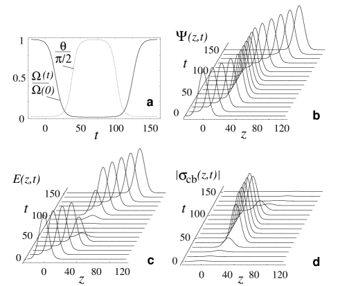
FIG. 3.: Propagation of a dark-state polariton with envelope $\exp\{-(z/10)^{2}\}$. The mixing angle is rotated from $0$ to $\pi/2$ and back according to $\cot\theta(t)=$ $100(1-0.5\tanh[0.1(t-15)]$ $+0.5\tanh[0.1(t-125)])$ as shown in (a). The coherent amplitude of the polariton $\Psi=\langle\hat{\Psi}\rangle$ is plotted in (b) and the electric field $E=\langle\hat{E}\rangle$ and matter components $|\sigma_{cb}|=|\langle\hat{\sigma}_{cb}\rangle|$ in (c) and (d) respectively. Axes are in arbitrary units with $c=1$.

D simultaneous narrowing of transparency window and pulse spectral width

As was discussed above, the transparency window of the EIT medium, i.e. the range of frequencies for which absorption is negligible, decreases with the group velocity. Since the bandwidth of the propagating pulse should always be contained within this range of frequencies to avoid absorption, the question arises whether this prevents the stopping of the polariton.

To answer this question we first note that during the process of adiabatic slowing the spatial profile, and in particular the length of the wavepacket ($\Delta l$) remains unaffected, as long as the group velocity is only a function of $t$. I.e.

$$\Delta l=\Delta l_{0}.$$ (72)

At the same time, the amplitude of the electric field gets reduced and its temporal profile stretched due to the reduction of the group velocity. The opposite happens when the group velocity is increased. One finds from eq.(67)

$$\hat{\cal E}(z,t)=\frac{\cos\theta(t)}{\cos\theta(0)}\,\hat{\cal E}\biggl{(}z-c\int^{t}_{0}\!\!\!{\rm d}\tau\cos^{2}\theta(\tau),0\biggr{)}.$$ (73)

As a consequence the spectrum of the probe field changes during propagation. Assuming that $\cos\theta$ changes only slow compared to the field amplitude one finds

$$S(z,\omega) = \frac{\cos^{2}\theta(t)}{\cos^{2}\theta(0)}S\left(0,\frac{\omega}{\cos^{2}\theta(t)}\right).$$ (74)

In particular the spectral width narrows (broadens) according to

$$\Delta\omega_{p}(t)\approx\Delta\omega_{p}(0)\,\frac{\cos^{2}\theta(t)}{\cos^{2}\theta(0)}.$$ (75)

When the group velocity of the polariton is reduced in time due to reduction of the control-field amplitude the EIT transparency window shrinks according to

$$\Delta\omega_{tr}(t)=\frac{\cot^{2}\theta(t)}{\cot^{2}\theta(0)}\Delta\omega_{tr}(0).$$ (76)

However the spectral width of the wavepacket shrinks as well and the ratio remains finite:

$$\frac{\Delta\omega_{p}(t)}{\Delta\omega_{tr}(t)}=\frac{\sin^{2}\theta(t)}{\sin^{2}\theta(0)}\frac{\Delta\omega_{p}(0)}{\Delta\omega_{tr}(0)}.$$ (77)

As will be discussed later on, for practically relevant cases, $\sin^{2}\theta(t)/\sin^{2}\theta(0)$ is always close to unity. Thus absorption can be prevented in the dynamic light-trapping method as long as the input pulse spectrum lies within the initial transparency window:

$$\Delta\omega_{p}(0)\ll\Delta\omega_{tr}(0).$$ (78)

As we have already noted earlier this condition can easily be fulfilled if an optically dense medium is used. The simultaneous reduction in transparency bandwidth and pulse bandwidth is illustrated in Fig.4.

FIG. 4.: Simultaneous narrowing of transmission spectrum (top) and pulse spectrum (bottom) for time dependent variation of group velocity $v/c$ in units of $\omega_{0}=g^{2}N/\gamma$. Parameters are $\alpha=20$, $g^{2}N/\gamma^{2}=10$.

E boundary behavior and initial pulse compression

In the above discussion we have analyzed the propagation of the probe pulse inside the medium. We now turn to the behavior at the medium boundaries. There are two issues of interest: (i) reflection from the medium surface and (ii) the effects of a possible steplike change of the group velocity when passing from vacuum or air to the medium.

Under ideal conditions the refractive index of the EIT medium is exactly unity on resonance and hence there is no reflection for the resonant component of the input pulse. If the spectrum of the input pulse is furthermore sufficiently narrow as compared to the initial transparency window of EIT, the refractive index is very close to unity over the entire relevant bandwidth and no field component gets reflected. To quantify this we note, that the index of refraction near resonance of an idealized, resonantly driven 3-level medium can be written as

$$n(\omega)\approx\sqrt{1+\frac{2c}{v_{g}^{0}}\frac{(\omega-\omega_{ab})}{\omega_{ab}}}.$$ (79)

The reflection coefficient for normal incidence from vacuum to the medium given by

$$R(\omega)=\left|\frac{1-n(\omega)}{1+n(\omega)}\right|^{2}$$ (80)

is plotted in fig.5.

FIG. 5.: Reflection coefficient for normal incidence as function of probe detuning from resonance.

Near resonance $R(\omega)$ can be approximated by

$$R(\omega)\approx\frac{\Delta\omega^{2}}{\Bigl{(}2\frac{v_{\rm g}^{0}}{c}\omega_{ab}+\Delta\omega\Bigl{)}^{2}}$$ (81)

where $\Delta\omega=\omega-\omega_{ab}$. Since typically $\Delta\omega_{p}(0)\ll\omega_{ab}\,v_{\rm g}^{0}/c$ reflection can be neglected.

When the group velocity inside the medium is smaller than c at the time when the probe pulse enters the medium, the pulse gets spatially compressed according to eq.(44). This substantially reduces the requirements on the size of the medium and enhances the storage capacity.

Continuity of the electric field amplitude ${\hat{\cal E}}$ at the entrance of the medium ($z=0$) implies a jump in the polariton amplitude

$$\hat{\Psi}(+0,t)=\sqrt{\frac{c}{v_{\rm g}^{0}}}\,\hat{\Psi}(-0,t)=\sqrt{\frac{c}{v_{\rm g}^{0}}}\,\,\hat{\cal E}(-0,t).$$ (82)

Hence the density of polaritons increases by a factor $c/v_{\rm g}$ when entering the medium, while there total number is conserved since the pulse length is changed by the inverse factor.

Boundary effects can also be used for a controlled deformation of a stored light pulse. When the polariton reaches the back end of the medium before $\cos\theta(t)$ approaches unity, the pulse will be spatially modulated.

V Limitations of quantum state-transfer

In the preceeding sections we have discussed the control of propagation of the photon wavepackets under the assumptions of an adiabatic evolution and small probe-field amplitudes. We furthermore neglected ground-state decoherence and motional (Doppler) effects. In the present section we will discuss the validity of these approximations in detail.

A non-adiabatic corrections

Let us first discuss the effect of non-adiabatic transitions i.e. let us take into account terms in first order of $\varepsilon$ in eqs.(63) and (65). For the following discussion it is sufficient to consider the semiclassical limit, where the operator character of the variables as well as the Langevin noise $F_{ba}$ can be disregarded. Up to $\varepsilon^{1}$ one obtains

$$\Phi\approx\sin^{2}\theta(t)\frac{\gamma}{g^{2}N}\,\dot{\theta}\,\Psi+\frac{\sin^{3}\theta(t)}{\cos\theta(t)}\frac{\gamma}{g^{2}N}\dot{\Psi}.$$ (83)

On the same level of approximations we can replace $\dot{\Psi}$ on the right hand side by $-c\cos^{2}\theta\partial\Psi/\partial z$. This gives

$$\Phi\approx\sin^{2}\theta(t)\frac{\gamma}{g^{2}N}\,\dot{\theta}\,\Psi-\sin^{3}\theta(t)\cos\theta(t)\frac{\gamma}{g^{2}N}c\frac{\partial}{\partial z}\Psi.$$ (84)

Substituting this into eq.(63) yields the lowest-order non-adiabatic corrections to the propagation equation of the dark-state polariton:

$$\left[\frac{\partial}{\partial t}+c\cos^{2}\theta(t)\frac{\partial}{\partial z}\right]\Psi(z,t)=-A(t)\Psi+B(t)c\frac{\partial}{\partial z}\Psi+$$ (85)

$$\quad\qquad+\,C(t)c^{2}\frac{\partial^{2}}{\partial z^{2}}\Psi-D(t)c^{3}\frac{\partial^{3}}{\partial z^{3}}\Psi,$$ (86)

where

$$A(t) = \Bigl{(}\gamma+\frac{1}{2}\frac{\partial}{\partial t}\Bigr{)}\left(\frac{\dot{\theta}^{2}\sin^{2}\theta}{g^{2}N}\right),$$ (87)

$$B(t) = \frac{\sin\theta}{3g^{2}N}\frac{\partial^{2}}{\partial t^{2}}\sin^{3}\theta,$$ (88)

$$C(t) = \Bigl{(}\gamma+\frac{1}{2}\frac{\partial}{\partial t}\Bigr{)}\frac{\sin^{4}\theta\cos^{2}\theta}{g^{2}N},$$ (89)

$$D(t) = \frac{\sin^{4}\theta\cos^{4}\theta}{g^{2}N}.$$ (90)

$A(t)$ describes homogeneous losses due to non-adiabatic transitions followed by spontaneous emission. $B(t)$ gives rise to a correction of the polariton propagation velocity, $C(t)$ results in a pulse spreading by dissipation of high spatial-frequency components and $D(t)$ leads to a deformation of the polariton.

Since all coefficients depend only on time, the propagation equation can be solved by a Fourier transform in space $\Psi(z,t)=\int{\rm d}k\,\widetilde{\Psi}(k,t)\,{\rm e}^{-ikz}$. This yields

$$\widetilde{\Psi}(k,t) = \widetilde{\Psi}(k,0)\,\exp\left\{ik\int_{0}^{t}\!\!\!{\rm d}t^{\prime}\Bigl{[}v_{\rm gr}(t^{\prime})+cB(t^{\prime})\Bigr{]}\right\}\times$$ (93)

$$\times\exp\left\{-ik^{3}c^{3}\int_{0}^{t}\!\!\!{\rm d}t^{\prime}D(t^{\prime})\right\}\times$$

$$\times\exp\left\{-\int_{0}^{t}\!\!\!{\rm d}t^{\prime}\Bigl{[}A(t^{\prime})+k^{2}c^{2}C(t^{\prime})\Bigr{]}\right\}.$$

The last term contains all losses due to non-adiabatic corrections. In order to neglect dissipation, the integral in the exponent of this term needs to be small compared to unity. Taking into account $\dot{\theta}(0)=\dot{\theta}(\infty)=0$ this results in the two conditions

$$\gamma k^{2}c^{2}\int_{0}^{\infty}\!\!{\rm d}t\,\frac{\sin^{4}\theta(t)\cos^{2}\theta(t)}{g^{2}N}\ll 1,$$ (94)

and

$$\gamma\int_{0}^{\infty}\!\!\!{\rm d}t\,\frac{\dot{\theta}^{2}\sin^{2}\theta}{g^{2}N}=\gamma\int_{0}^{\infty}\!\!\!{\rm d}t\,\frac{\dot{\theta}^{2}}{g^{2}N+\Omega^{2}(t)}\ll 1.$$ (95)

The first condition can be brought into a transparent form when replacing $\sin^{4}\theta$ by unity, which results in

$$\gamma k^{2}c^{2}\int_{0}^{\infty}\!\!{\rm d}t\,\frac{\cos^{2}\theta(t)}{g^{2}N}=\frac{\gamma k^{2}cz}{g^{2}N}\ll 1$$ (96)

for all relevant $k$. Here $z=c\int_{0}^{\infty}{\rm d}t\,\cos^{2}\theta(t)$ is the propagation depth of the polariton inside the medium, and we have assumed $\cos\theta(0)=1$ and $\cos\theta(\infty)=0$ for simplicity. Noting that the range of relevant spatial Fourier frequencies is determined by the inverse of the initial pulse length $L_{p}$, i.e. setting $k\sim L_{p}^{-1}$, one finds

$$z\ll\frac{g^{2}N}{\gamma c}\,L_{p}^{2}\quad{\rm or}\quad z\ll\sqrt{\alpha}L_{p},$$ (97)

where $\alpha=g^{2}Nz/\gamma c$ is again the opacity of the medium without EIT. To illustrate this limitation we have shown in Fig.6 the slow-down and successive acceleration of a light pulse obtained from a numerical solution of the full 1-d propagation problem as well as the analytical approximation following from eq.(93). Here $\frac{g^{2}N}{\gamma c}\frac{L_{p}^{2}}{z_{\rm max}}=2$  ($z_{\rm max}=250$). One clearly recognizes a decay of the elm. excitation $E$ long before the deceleration and the associated transfer to the atom systems sets in. The polariton energy $I_{\Psi}\equiv\int{\rm d}z|\Psi(z,t)|^{2}$ decreases approximately exponentially with the propagation distance $\Delta z$ of the pulse center. In the example $I_{\Psi}$ decays after $\Delta z=250$ approximately by a factor ${\rm e}^{-0.322}\approx 0.724$.

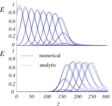
FIG. 6.: Deceleration (top) and re-aceleration (bottom) of a Gaussian light pulse $\exp[-(t-500)^{2}/(200)^{2}]$ with $\cot\theta(t)=0.363\bigl{(}1-(2/\pi)\,{\rm arccot}[5(1-0.5\tanh[0.005(t-2000)]$ $+0.5\tanh[0.005*(t-3200)])]\bigr{)}$. The parameters are $g^{2}N/\gamma^{2}=2.5,\alpha=625,c=1$. Pulses are shown for $t=$600, 800, 1000, 1200, 1400, 1600, 1800, 2000, 2200, and 2400 in the top figure and for $t=$2800, 3000, 3200, 3400, 3800, 4000 in the bottom figure. One recognizes good agreement between numerical solution of the propagation equations (solid line) and analytic approximation (dashed line).

Since the spatial pulse length in the medium is related to the initial group velocity $v_{g}^{0}$ (at time $t=0$ before the trapping) and to the initial pulse bandwidth as $L_{p}\sim v_{g}^{0}/\Delta\omega_{p}(0)$ and since $\Delta\omega_{tr}(0)=\sqrt{\alpha}/\tau_{d}\approx\sqrt{\alpha}v_{g}^{0}/z$, for $v_{g}^{0}\ll c$, equation (97) is simply another way to state:

$$\Delta\omega_{p}\ll\Delta\omega_{tr}(0).$$ (98)

Hence the present analysis confirms the qualitative conditions for adiabatic following: the initial probe spectrum should be contained within the original transparency window. Once again, this can be satisfied if the medium is optically dense, $\alpha\gg 1$.

There is also a second condition (95) which is well-known from adiabatic passage requirement [29, 34] and sets a limit to the rotation velocity $\dot{\theta}$ of the mixing angle and hence to the deceleration/acceleration of the polariton. Introducing a characteristic time scale of the acceleration/deceleration period $T$ we obtain

$$T>{l_{abs}\over c}{v_{g}^{0}\over c},$$ (99)

where $l_{abs}=c\gamma/g^{2}N$ is the absorption length in the absence of EIT. We note that for realistic experimental parameters the quantity on the right hand side is extremely small on all relevant time scales. Hence, in practice the rate of change of the mixing angle does not significantly affect the adiabatic dynamics.

B weak field approximation

The analysis of sec.IV also involves a perturbation expansion, valid when the control field is much stronger than the probe field. It is easy to see that this expansion is justified even when the control-field Rabi-frequency is reduced to zero. Making use of (36) one finds: $g^{2}\langle{\hat{E}}^{+}{\hat{E}}\rangle/|\Omega|^{2}=\langle{\hat{\sigma}}_{cb}{\hat{\sigma}}_{bc}\rangle=\langle\hat{\sigma}_{cc}\rangle$. I.e., the ratio of the average intensities of quantum and control field is proportional to the probability to find an atom in state $c$. If the initial number-density of photons in the quantum field is much less than the number-density of atoms, $\langle\hat{\sigma}_{cc}\rangle$ is always much smaller than unity. Therefore the mean intensity of the quantum field remains small compared to that of the control field even when the latter is turned to zero.

C decay of Raman coherence

In the ideal scenario considered in sec.IV we disregarded all processes resulting in a decay of coherences between the metastable states $b$ and $c$. If such a decay at a rate $\gamma_{0}$ is taken into account, the group velocity in the EIT medium cannot reach zero. Nevertheless an (almost) complete transfer of the quantum state of a propagating light pulse to a stationary matter excitation is possible. Introducing phenomenogical decay into the equation of the Raman coherence ${\hat{\sigma}}_{bc}$ results in a modification of equation (32) according to

$${\widetilde{\sigma}}_{ba}=-\frac{i}{\Omega^{*}}{\rm e}^{i\Delta kz}\left(\frac{\partial}{\partial t}{\widetilde{\sigma}}_{bc}+\gamma_{0}{\widetilde{\sigma}}_{bc}\right)+F_{bc}.$$ (100)

For formal consistency a Langevin noise term associated with the decoherence needed to be introduced as well. Such a dephasing trivially modifies the propagation law of the polariton

$$\hat{\Psi}(z,t) = \exp\Bigl{(}-\gamma_{0}\int_{0}^{t}\!\!d\tau\sin^{2}\theta(\tau)\Bigr{)}\times$$ (102)

$$\times\hat{\Psi}\biggl{(}z-c\int^{t}_{0}\!\!\!{\rm d}\tau\cos^{2}\theta(\tau),0\biggr{)}+{\hat{F}}_{\Psi}.$$

As expected dephasing simply results in a decay of the polartion amplitude $\langle\hat{\Psi}\rangle$ but does not prevent light stopping. A more detailed discussion of various realistic decoherence mechanisms and their influence on the fidelity of the quantum memory will be presented in a subsequent publication.

D atomic motion

We have shown above that adiabatically varying the envelope of the control field $\Omega$ in time a light pulse of the probe field can be brought to a full stop. A spatially homogeneous variation of the group velocity can be realized, for instance, in the case when the control and probe field are propagating in orthogonal directions. However, in such a case the spin-wave component of the polariton has a phase, which is rapidly oscillating in $z$, since then $\Delta k=k_{d}-k_{d}^{\parallel}=k_{d}(1-\cos\theta)=k_{d}$. For an atom at position $z_{j}$ one would have

$$\hat{\sigma}_{bc}^{j}(t)=|\hat{\sigma}_{bc}^{j}(t)|\,\exp\left\{i\frac{\omega_{ac}}{c}z_{j}\right\}\exp\left\{-i\frac{\omega_{bc}}{c}z_{j}\right\},$$ (103)

where a transformation from the rotating frame back into the lab frame was applied. While the second term corresponds to spatial oscillations with the small beat-frequency between pump and drive, the first term oscillates with an optical frequency. As a consequence the the polariton state is highly sensitive to variations in the atomic positions, or in other words would dephase rapidly due to atomic motion. To retain a high fidelity of the quantum memory it would be necessary to confine the motion of the atoms during the storage time to within a fraction of an optical wavelength, which is a very stringent condition.

To avoid this problem nearly co-propagating beams can be used, such that $\Delta k\ll k_{d}$. In this case almost no photonic momentum is transferred to the atoms and the two-photon transition frequency would experience only a very small Doppler-shift. Such a configuration is therefore robust with respect to atomic motion, as electronic and motional degrees of freedom are completely decoupled.

In a Doppler-free configuration propagation effects of the control field need to be considered. In the case when the probe field is weak compared to the control field at all times, the latter propagates almost as in free space and $\Omega(z,t)=\Omega(t-z/c)$. Due to the resulting $z$-dependence of the group velocity, the trapping mechanism does not exactly preserve the shape of the photon wavepacket. However, when the probe pulse enters the medium with a group velocity much smaller than the velocity of the control field $v_{g}^{0}\ll c$, the retardation of the control-field amplitude can be ignored and $\Omega(t-z/c)\approx\Omega(t)$. This is a good approximation as long as the time variation of the control field is sufficiently slow such that its spatial variation across the probe pulse length is small. This implies that the characteristic time of change of the control field should obey ${T}\gg L_{p}/c$, which is again easily satisfied.

Before concluding we note that even in the case when no photon momentum is transfered to atoms and therefore atomic motion does not result in altering the phase of the spin coherence, in practice it is still desirable to suppress the motion. This is because the light beams normally have a finite cross-section and the atomic coherence is localized in the longitudinal direction and motion would tend to spread the localized excitation over the entire volume occupied by the gas. In this case the information about the pulse shape and the mode function will be lost after a sufficiently long storage interval. That is the reason why techniques involving cold trapped atoms and buffer gas were used to effectively slow the atomic drifts in recent experiments [20, 21].

VI summary

In conclusion we introduced the basic idea of quantum memory for light based on dark-state polaritons and discussed their properties. We have considered the influence of the main realistic imperfections on trapping and re-acceleration and have shown that the technique is extremely robust. In particular, we demonstrated that an essential mechanism that enables the efficient quantum memory operation - the adiabatic following in polaritons - can take place despite of transparency window narrowing. Subsequent papers will discuss the influence of other decoherence mechanisms on photon trapping and retrieval and will present the results of detail numerical simulations of the trapping procedure.

REFERENCES

- [1] D. P. DiVincenzo, Science 270, 255 (1995); C. H. Bennett, Phys. Today 48, No. 10, 24 (1995); A. Ekert and R. Josza, Rev. Mod. Phys. 68, 733 (1996); J. I. Cirac and P. Zoller, Phys. Rev. Lett. 74, 4091 (1995).
- [2] C. H. Bennett and G. Brassard, Proc. of IEEE Int. Conf. on Comp. Systems and Signal Processing, Banglore India (IEEE, New York 1984); A. K. Ekert, Phys. Rev. Lett. 67, 661 (1991).
- [3] C. H. Bennett et al., Phys. Rev. Lett. 70, 1895 (1990); B. Bouwmeester et al., Nature 390, 575 (1997); D. Boschi et al., Phys. Rev. Lett. 80, 1121 (1998); A. Furusawa et al. Science 282, 706 (1998).
- [4] D.P. DiVincenzo, Fortschr. Physik, 48, 771 (2000).
- [5] E. L. Hahn, Phys. Rev. 80, 580 (1950).
- [6] J. D. Abella, N. A. Kurnit, and S. R. Hartmann, Phys. Rev. 141, 391 (1966).
- [7] T. W. Mossberg, Opt. Lett. 7, 77 (1982).
- [8] N. W. Carlson, L. J. Rothberg, A. G. Yodh, W. R. Babbitt, and T. W. Mossberg, Opt. Lett. 8, 483 (1983).
- [9] K.P. Leung, T. W. Mossberg and S. R. Hartmann, Opt. Comm. 43, 145 (1982).
- [10] P.R. Hemmer, K. Z. Cheng, J. Kierstead, M. S. Shariar, and M. K. Kim, Opt. Lett. 19, 296 (1994); B. S. Ham, M. S. Shariar, M. K. Kim, and P. R. Hemmer, Opt. Lett. 22, 1849 (1997).
- [11] A. S. Parkins, P. Marte, P. Zoller and H. J. Kimble, Phys. Rev. Lett. 71, 3095 (1993); T. Pelizzari, S. A. Gardiner, J. I. Cirac, and P. Zoller, Phys.Rev.Lett. 75, 3788 (1995); J. I. Cirac, P. Zoller, H. Mabuchi and H. J. Kimble, Phys.Rev.Lett. 78, 3221 (1997).
- [12] K. Bergmann, H. Theuer, and B. W. Shore, Rev. Mod. Phys. 70, 1003 (1998); N. V. Vitanov, M. Fleischhauer, B. W. Shore, and K. Bergmann, Adv. Atom. Mol. Opt. Physics (2001) (in press).
- [13] H. J. Kimble, Physica Scripta, 76, 127 (1998).
- [14] A. Kuzmich, K. Mølmer, and E. S. Polzik, Phys. Rev. Lett. 79, 4782 (1997), J. Hald, J. L. Sørensen, C. Schori, and E. S. Polzik, Phys. Rev. Lett. 83, 1319 (1999).
- [15] A. E. Kozhekin, K. Mølmer, E. Polzik Phys. Rev. A 62, 033809 (2000).
- [16] M. D. Lukin, S. F. Yelin, and M. Fleischhauer, Phys. Rev. Lett., 84, 4232 (2000);
- [17] M. Fleischhauer and M. D. Lukin, Phys. Rev. Lett. 84, 5094 (2000);
- [18] M. Fleischhauer, S. F. Yelin, and M. D. Lukin, Opt. Comm. 179, 395 (2000).
- [19] S. E. Harris, Physics Today 50, 36 (1997).
- [20] C. Liu, Z. Dutton, C.H. Behroozi, and L.V. Hau, Nature 409, 490 (2001).
- [21] D. F. Phillips, A. Fleischhauer, A. Mair, R. L. Walsworth, and M. D. Lukin, Phys. Rev. Lett. 86, 783 (2001).
- [22] L. V. Hau, S. E. Harris, Z. Dutton, and C. H. Behroozi, Nature 397, 594 (1999); M. Kash et al. Phys. Rev. Lett. 82, 5229 (1999); D. Budker et al. Phys. Rev. Lett. 83, 1767 (1999).
- [23] S. E. Harris, L. V. Hau, Phys. Rev. Lett. 82, 4611 (1999);
- [24] M. D. Lukin, M. Fleischhauer, A. S. Zibrov, H. G. Robinson, V. L. Velichansky, L. Hollberg, and M.O. Scully, Phys. Rev. Lett. 79 , 2959 (1997).
- [25] I. E. Mazets, and B. G. Matisov, JETP Lett. 64, 515 (1996) [Pisma, Zh. Exp. Teor. Fiz. 64, 473 (1996)].
- [26] J. R. Csesznegi and R. Grobe, Phys. Rev. Lett. 79, 3162 (1997).
- [27] R. H. Dicke, Phys. Rev. 93, 99 (1954).
- [28] M. D. Lukin, M. Fleischhauer, M. O. Scully, and V. L. Velichansky, Opt. Lett. 23 , 295 (1998)
- [29] M. Fleischhauer and A.S. Manka, Phys. Rev. A 54 , 794 (1996).
- [30] M. D. Lukin, A. Imamoğlu, Phys. Rev. Lett. 84, 1419 (2000).
- [31] see e.g.: E. Arimondo, Progr. in Optics 35, 259 (1996);
- [32] O. Kocharovskaya, Y. Rostovtsev, M.O. Scully, Phys. Rev. Lett. 86, 628 (2001).
- [33] U. Leonhardt and P. Piwnicki, Phys. Rev. Lett. 84, 822 (2000).
- [34] N. V. Vitanov and S. Stenholm, Opt. Comm. 127, 215 (1996); N. V. Vitanov and S. Stenholm, Phys. Rev. A 56, 1463 (1997);